On the Universality of the Energy Response Function in the Long-Range Spin Glass Model with Sparse, Modular Couplings

Abstract

We consider energy relaxation of the long-range spin glass model with sparse couplings, the so-called dilute Sherrington-Kirkpatrick (SK) model, starting from a random initial state. We consider the effect that modularity of the coupling matrix has on this relaxation dynamics. In the absence of finite size effects, the relaxation dynamics appears independent of modularity. For finite sizes, a more modular system reaches a less favorable energy at long times. For small system sizes, a more modular system also has a less favorable energy at short times. For large system sizes, modularity may lead to slightly more favorable energies at intermediate times. We discuss these results in the context of evolutionary theory, where horizontal gene transfer, absent in the Glauber equilibration dynamics of the SK model studied here, endows modular organisms with larger response functions at short times.

I Introduction

We here consider energy relaxation in a dilute, modular spin glass. The form of the energy function, its sparseness and modularity, is motivated by fitness functions encountered in biology He et al. (2009); Lorenz et al. (2011); Clune et al. (2013); Friedlander et al. (2013). We emphasize that our calculation is one of statistical mechanics, rather than of a detailed evolutionary model. The model is similar in spirit to the spin-glass models that have been introduced to analyze the relation between genotype and phenotype evolution Anderson (1983); Kauffman and Levin (1987); Sakata et al. (2009, 2012). The model is also quite similar to a model of associate memory recall, in which modularity was shown to increase the rate of pattern matching Pradhan et al. (2011). Multi-body contributions to the fitness function in biology, leading to a rugged fitness landscape and glassy evolutionary dynamics, are increasingly thought to be an important factor in evolution Breen et al. (2012). That is, biological fitness functions may be characterized as instances of fitness functions taken from a spin glass ensemble. Importantly, though, biological fitness functions have a modular structure, and their dependence on the underlying variables is somewhat separable Bogarad and Deem (1999); Sun et al. (2005a, 2006). Glassy evolutionary dynamics has been noted a number of times Khatri et al. (2009); Vetsigian et al. (2006). The generalized NK model used to understand the immune response to vaccines and evolving viruses is a type of modular, dilute spin glass model Deem and Lee (2003); Park and Deem (2004); Sun et al. (2005b); Zhou and Deem (2006); Gupta et al. (2006); Yang et al. (2006); Pan and Deem (2011).

We here analyze, within the context of statistical mechanics rather than a detailed evolutionary model, the dependence of a spin glass response function on the modularity of the interactions. We consider how the spin glass equilibrates from an initially random state by Glauber dynamics. At long times, the finite-size corrections to the energy per spin in the SK spin glass scale as $L^{-2/3}$, where $L$ is the system size G. Parisi and Slanina (1993a, b); Billoire (2006); Aspelmeier et al. (2008). The timescale for convergence, $t_{\rm ERG}$ grows exponentially with system size, $t_{\rm ERG}\sim t_{0}\exp(cL^{1/3})$ Bouchaud et al. (1998); Kinzelbach and Horner (1991); Bittner et al. (2008); Dotsenko (1985).

Here, we derive the approximate response function at short times. Since modularity is a relevant, emergent order parameter in dynamical systems Waddington (1942); Simon (1962); Hartwell et al. (1999); Kashtan et al. (2009); Wagner et al. (2007); Sun and Deem (2007), we consider the ensemble of spin glass Hamiltonians parametrized by modularity, $M$. In particular, we make predictions for how the energy relaxation of a dilute spin glass depends on the modularity of the coupling matrix. Numerical calculations have shown that the energy per spin relaxes at different rates for spin glass systems of different sizes Kinzel (1986), and these simulations provide additional motivation for the present calculations.

In a replica calculation, we will show that the response function at short times is independent of modularity for large system sizes. This calculation generalizes the dynamical equations of magnetization and energy Coolen and Sherrington (1994) to the dilute SK model and determines the form that these equations take near the spin glass phase transition. The universality of the response function may be broken by finite size effects. At long times, greater modularity leads to less favorable energies due to these finite size effects. Near the spin glass transition, there are two opposing finite size effects, and greater modularity may lead to a slightly more rapid energy decay.

The rest of the paper is organized as follows. In Section II we describe simple scaling arguments for the energy relaxation curve at short and long times as a function of modularity. In Section III we introduce the dilute, modular SK model and the projection of the energy dynamics onto the slow modes. In Section IV we derive the slow mode dynamics by a replica approach. In Section V we analyze these equations to produce the energy relaxation curve. In Section VI we use known thermodynamic finite scaling results to argue how the dynamical equations depend on system size. In Section VII we compare the results to numerical calculations. We discuss these results in Section VIII and conclude in Section IX.

II Modularity as a Finite Size Effect

We consider a spin glass with long range couplings. The entries in the $N\times N$ coupling matrix are symmetrically distributed around zero, and the sum of the variances of the couplings in each row is $O(1)$. We contrast this case where every entry of the matrix may be nonzero to the case where only the entries along the $L\times L$ block diagonals may be nonzero. This latter case is an example of a modular coupling matrix. The parameter $L$ is a measure of the effective modularity in the system, with smaller $L$ indicating greater effective modularity.

A system with smaller $L$ has a less favorable ground state energy. In particular, if we set the negative of the energy per spin to be $r$, it is known that $r^{*}=r_{\infty}-aL^{-2/3}$ Aspelmeier et al. (2008). The value of $K$ in the Parisi hierarchy required to stabilize a system of size $L$ grows as $K\sim(T_{c}-T)L^{1/6}$, where $T$ is temperature Aspelmeier et al. (2008). This result can be used to estimate finite effects if observables are known as a function of $K$. In our case, arguing that the barriers to equilibration of a larger system further down in the Parisi hierarchy are of the same order as the energy of the smaller system from the $K\to\infty$ ground state, $\Delta E\sim N(r_{\infty}-r^{*})$, we would expect $t_{\rm ERG}\sim t_{0}\exp(cL^{1/3})$ Bouchaud et al. (1998); Kinzelbach and Horner (1991); Bittner et al. (2008). We expect logarithmic convergence to the ground state at long time Dotsenko (1985). Smoothing the short time behavior, the scaled energy might follow $r_{L}(t)=r_{\infty}-aL^{-2/3}\tanh t-b[1+\ln(1+t/t_{\rm ERG})]^{-2/\nu}$, where $\nu=1$ to have the expected $L$ dependence at large time, and $a$ and $b$ are constants of order unity. The long time ordering of these curves with $L$ is a result of equilibrium finite size effects. Whether the curves cross at short time depends on the details of the equilibration dynamics and is the subject of the rest of this paper.

The rest of this article will calculate the short time behavior of the energy relaxation curve for a class of coupling matrices that interpolate between the fully connected $N\times N$ matrix and one with $L\times L$ block diagonals. The modularity order parameter, $M$, is zero in the first case and unity in the second.

III Model

The focus of the present study is how to introduce modularity to the SK model, and the resulting short-time dynamics. The coupling matrix must have local structure, and it must be sparse, as modularity can not be identified in a fully connected matrix. A visual depiction of the non-zero entries in coupling matrix is shown in Fig. 1.

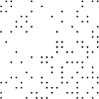
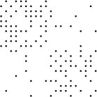
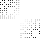
Figure 1: Shown is a simplified view of the couplings in the dilute SK model. In this figure, we consider a system of size $N=20$. If spin $i$ interacts with spin $j$, a dot is displayed at matrix position $i,j$. Each position $i$ interacts on average with $C$ other positions. Here $C=6$. Left) A non-modular structure, $M=0$. Middle) A moderately modular structure, $M=2/3$. Right) A fully modular structure, $M=1$. The matrix shown here is the connection matrix, denoted by the symbol $\Delta$. Here, there are two modules, each of size $L=10$. We define modularity from the excess number of interactions within the two $L\times L$ block diagonals over that expected based upon the probability observed outside the block diagonals. This number is divided by the total number of interactions to give the modularity, $M$.

We define a spin glass model that generically incorporates sparseness and modularity. The connection matrix for a given system $\alpha$ is denoted by $\Delta^{\alpha}$ with $\Delta^{\alpha}_{ij}=0,1$, as shown in Fig. 1. Each spin $i$ is connected to $C$ other spins, on average. Putting these points together, our simplified model is a dilute SK model:

$$H^{\alpha}(\{\sigma\})=-\sum_{i<j}J_{ij}\sigma_{i}\sigma_{j}\Delta_{ij}^{\alpha}$$ (1)

with $J_{ij}=Jz_{ij}$ where z is a quenched Gaussian with zero mean and variance $1/C$. The number $C$ is the average number of connections, and so in the absence of modularity $P(\Delta_{ij})=(1-C/N)\delta_{\Delta_{ij},0}+(C/N)\delta_{\Delta_{ij},1}$. We have $\sigma_{i}=\pm 1$. The spin dynamics is governed by Glauber dynamics such that the rate to flip spin $k$ in the sequence is given by $w_{k}(\{\sigma\})=\frac{1}{2}(1-\sigma_{k}\tanh\beta h_{k})$ where $h_{k}=\sum_{j\neq k}J_{kj}\Delta_{kj}\sigma_{j}=Jz_{k}$, with $z_{k}=\sum_{j\neq k}z_{kj}\Delta_{kj}\sigma_{j}$.

Now we generalize this model by introducing modularity, such that there is an excess of interactions in $\Delta$ along the $L\times L$ block diagonals of the $N\times N$ connection matrix. There are $k_{1}=N/L$ of these block diagonals. Thus, the probability of a connection is $C_{0}/N$ when $\lfloor i/L\rfloor\neq\lfloor j/L\rfloor$ and $C_{1}/N$ when $\lfloor i/L\rfloor=\lfloor j/L\rfloor$. The number of connections is $C=C_{0}+(C_{1}-C_{0})/k_{1}$. Modularity is defined by $M=(C_{1}-C_{0})/(k_{1}C)$. To see the spin glass phase, the system must be macroscopic, $N\to\infty$. In addition, the module size must be large, so that the glass phase appears. We also require $C$ is large so that the spin glass remains mean field.

We define the total magnetization $m=(1/N)\sum_{i=1}^{N}\sigma_{i}$ and scaled energy per spin $r=-H/(JN)$. We split the energy per spin into a component inside the block diagonals and a component outside: $r_{I}=-\sum_{i<j,\lfloor i/L\rfloor=\lfloor j/L\rfloor}J_{ij}\sigma_{i}\sigma_{j}\Delta_{ij}^{\alpha}$, and $r_{O}=-\sum_{i<j,\lfloor i/L\rfloor\neq\lfloor j/L\rfloor}J_{ij}\sigma_{i}\sigma_{j}\Delta_{ij}^{\alpha}$, with $r=r_{I}+r_{O}$. We also define $z_{k}^{I}=\sum_{j\neq k,\lfloor j/L\rfloor=\lfloor k/L\rfloor}z_{kj}\Delta_{kj}\sigma_{j}$ and $z_{k}^{O}=\sum_{j\neq k,\lfloor j/L\rfloor\neq\lfloor k/L\rfloor}z_{kj}\Delta_{kj}\sigma_{j}$. We project the microscopic probability of a given state, $P_{t}(\sigma)$, onto these order parameters. These order parameters evolve according to Coolen and Sherrington (1994) (see Eqs. 8 and 9 therein)

$$\frac{dm}{dt} =\int dxdyD_{m,r_{I},r_{O};t}[x,y]\tanh\beta J(x+y)-m$$

$$\frac{dr_{I}}{dt} =\int dxdyD_{m,r_{I},r_{O};t}[x,y]x\tanh\beta J(x+y)-2r_{I}$$

$$\frac{dr_{O}}{dt} =\int dxdyD_{m,r_{I},r_{O};t}[z,y]y\tanh\beta J(x+y)-2r_{O}$$ (2)

where

$$D_{m,r_{I},r_{O};t}[x,y] = \lim_{N\to\infty}\sum_{\sigma}P_{t}(\sigma)\delta([m-m(\sigma)]\delta[r_{I}-r_{I}(\sigma)]\delta[r_{O}-r_{O}(\sigma)]$$ (3)

$$\times\frac{\frac{1}{N}\sum_{k=1}^{N}\delta[x-z_{k}^{I}(\sigma)]\delta[y-z_{k}^{O}(\sigma)]}{\sum_{\sigma^{\prime}}P_{t}(\sigma^{\prime})\delta([m-m(\sigma^{\prime})]\delta[r_{I}-r_{I}(\sigma^{\prime})]\delta[r_{O}-r_{O}(\sigma^{\prime})]}$$

We assume that $D_{m,r_{I},r_{O};t}[x,y]$ is self-averaging over the disorder, which numerical simulations out to intermediate times seem to support Coolen and Sherrington (1994). We will also assume equipartitioning of probability in the macroscopic subshell $(m,r_{I},r_{O})$ Coolen and Sherrington (1994). These assumptions allow us to drop $P_{t}(\sigma)$ and to perform the averages over the quenched random $z_{ij}$ and $\Delta_{ij}$ variables:

$$D_{m,r_{I},r_{O};t}[x,y] = \lim_{N\to\infty}\bigg{\langle}\sum_{\sigma}\delta[m-m(\sigma)]\delta[r_{I}-r_{I}(\sigma)]\delta[r_{O}-r_{O}(\sigma)]$$ (4)

$$\times\frac{\frac{1}{N}\sum_{k=1}^{N}\delta[x-z_{k}^{I}(\sigma)]\delta[y-z_{k}^{O}(\sigma)]}{\sum_{\sigma^{\prime}}\delta[m-m(\sigma^{\prime})]\delta[r_{I}-r_{I}(\sigma^{\prime})]\delta[r_{O}-r_{O}(\sigma^{\prime})]}\bigg{\rangle}_{\{z_{ij}\},\{\Delta_{ij}\}}$$

IV Replica Analysis

We now proceed to analytically calculate the averages required to determine the solution to Eq. (2). We define $w(\sigma)=\delta([m-m(\sigma)]\delta[r_{I}-r_{I}(\sigma)]\delta[r_{O}-r_{O}(\sigma)]$. We use the replica expression in the form

$$\langle\Phi(\sigma)\rangle_{w} = \frac{{\rm Tr}_{\sigma}w(\sigma)\Phi(\sigma)}{{\rm Tr}_{\sigma}w(\sigma)}$$ (5)

$$= \frac{{\rm Tr}_{\sigma^{1}\ldots\sigma^{n}}w(\sigma^{1})\Phi(\sigma^{1})w(\sigma^{2})\cdots w(\sigma^{n})}{{\rm Tr}_{\sigma^{1}\ldots\sigma^{n}}w(\sigma^{1})\cdots w(\sigma^{n})}$$

$$= \frac{{\rm Tr}_{\sigma^{1}\ldots\sigma^{n}}w(\sigma^{1})\Phi(\sigma^{1})w(\sigma^{2})\cdots w(\sigma^{n})}{[{\rm Tr}_{\sigma}w(\sigma)]^{n}}$$

$$= \lim_{n\to 0}\frac{{\rm Tr}_{\sigma^{1}\ldots\sigma^{n}}w(\sigma^{1})\Phi(\sigma^{1})w(\sigma^{2})\cdots w(\sigma^{n})}{[{\rm Tr}_{\sigma}w(\sigma)]^{n}}$$

$$= \lim_{n\to 0}{\rm Tr}_{\sigma^{1}\ldots\sigma^{n}}w(\sigma^{1})\Phi(\sigma^{1})w(\sigma^{2})\cdots w(\sigma^{n})$$

to write

$$D_{m,r_{I},r_{O};t}[x,y] = \lim_{N\to\infty}\lim_{n\to 0}\frac{1}{N}$$

$$\sum_{k=1}^{N}\left\langle{\rm Tr}_{\sigma^{1}\ldots\sigma^{n}}\delta[x-z_{k}^{I}(\sigma^{1})]\delta[y-z_{k}^{O}(\sigma^{1})]w(\sigma^{1})w(\sigma^{2})\cdots w(\sigma^{n})\right\rangle_{\{z_{ij}\},\{\Delta_{ij}\}}$$

Using the Fourier representation of the delta function, we find Coolen and Sherrington (1994)

$$D_{m,r_{I},r_{O}}[x,y] = \lim_{N\to\infty}\lim_{n\to 0}\frac{1}{N}\sum_{k=1}^{N}\int\frac{d\xi d\eta}{(2\pi)^{2}}\left[\prod_{\alpha=1}^{n}\frac{Nd\tilde{m}_{\alpha}}{2\pi}\frac{Nd\tilde{r}_{\alpha}^{I}Nd\tilde{r}_{\alpha}^{O}}{(2\pi)^{2}}\right]e^{i\xi x+i\eta y}$$

$${\rm Tr}_{\sigma}e^{iN\sum_{\alpha}[\tilde{m}_{\alpha}(m-m(\sigma))+\tilde{r}_{\alpha}^{I}r_{I}+\tilde{r}_{\alpha}^{O}r_{O}]}$$

$$\times\left\langle e^{-i\xi\sum_{j\neq k}^{I}z_{kj}\sigma_{j}^{1}\Delta_{kj}-i\eta\sum_{j\neq k}^{O}z_{kj}\sigma_{j}^{1}\Delta_{kj}-i\sum_{\alpha}\tilde{r}_{\alpha}^{I}\sum_{i<j}^{I}z_{ij}\sigma_{i}^{\alpha}\sigma_{j}^{\alpha}\Delta_{ij}-i\sum_{\alpha}\tilde{r}_{\alpha}^{O}\sum_{i<j}^{O}z_{ij}\sigma_{i}^{\alpha}\sigma_{j}^{\alpha}\Delta_{ij}}\right\rangle_{\{z_{ij}\},\{\Delta_{ij}\}}$$

where in the limits of the sum we have used the notation $I$ for restriction inside the block diagonals and $O$ to restriction outside the block diagonals. We average the quantity in brackets over the $\Delta_{ij}$, setting $k=1$ by permutation symmetry to find

$$\prod_{j=2}^{L}\left[\left(1-\frac{C_{1}}{N}\right)+\frac{C_{1}}{N}e^{-i\xi z_{1j}\sigma_{j}^{1}-i\sum_{\alpha}\tilde{r}_{\alpha}^{I}\sigma_{1}^{\alpha}z_{1j}\sigma_{j}^{\alpha}}\right]$$

$$\prod_{j=L+1}^{N}\left[\left(1-\frac{C_{0}}{N}\right)+\frac{C_{0}}{N}e^{-i\eta z_{1j}\sigma_{j}^{1}-i\sum_{\alpha}\tilde{r}_{\alpha}^{O}\sigma_{1}^{\alpha}z_{1j}\sigma_{j}^{\alpha}}\right]$$

$$\prod_{1<i<j}^{I}\left[\left(1-\frac{C_{1}}{N}\right)+\frac{C_{1}}{N}e^{-i\sum_{\alpha}\tilde{r}_{\alpha}^{I}\sigma_{i}^{\alpha}z_{ij}\sigma_{j}^{\alpha}}\right]$$

$$\prod_{1<i<j}^{O}\left[\left(1-\frac{C_{0}}{N}\right)+\frac{C_{0}}{N}e^{-i\sum_{\alpha}\tilde{r}_{\alpha}^{O}\sigma_{i}^{\alpha}z_{ij}\sigma_{j}^{\alpha}}\right]$$ (8)

Recognizing that $C_{0}/N$ and $C_{1}/N$ are small, so that the above expression can be written in exponential form, Eq. (LABEL:4a) becomes

$$D_{m,r_{I},r_{O}}[x,y]=\lim_{N\to\infty}\lim_{n\to 0}\frac{1}{N}\sum_{k=1}^{N}\int\frac{d\xi d\eta}{(2\pi)^{2}}\left[\prod_{\alpha=1}^{n}\frac{Nd\tilde{m}_{\alpha}}{2\pi}\frac{Nd\tilde{r}_{\alpha}^{I}}{2\pi}\frac{Nd\tilde{r}_{\alpha}^{O}}{2\pi}\right]e^{i\xi x+i\eta y}$$

$${\rm Tr}_{\sigma}e^{iN\sum_{\alpha}[\tilde{m}_{\alpha}(m-m(\sigma))+\tilde{r}_{\alpha}^{I}r_{I}+\tilde{r}_{\alpha}^{O}r_{O}]}$$

$$e^{\frac{C_{1}}{N}\sum_{i<j}^{I}\left(\left\langle\exp(-i\sum_{\alpha}\tilde{r}_{\alpha}^{I}\sigma_{i}^{\alpha}z_{ij}\sigma_{j}^{\alpha})\right\rangle_{\{z_{ij}\}}-1\right)}$$

$$e^{\frac{C_{0}}{N}\sum_{i<j}^{O}\left(\left\langle\exp(-i\sum_{\alpha}\tilde{r}_{\alpha}^{O}\sigma_{i}^{\alpha}z_{ij}\sigma_{j}^{\alpha})\right\rangle_{\{z_{ij}\}}-1\right)}$$

$$e^{\frac{C_{1}}{N}\sum_{j=2}^{L}\left(\left\langle\exp(-i\xi z_{1j}\sigma_{j}^{1}-i\sum_{\alpha}\tilde{r}_{\alpha}^{I}\sigma_{1}^{\alpha}z_{1j}\sigma_{j}^{\alpha})\right\rangle_{\{z_{ij}\}}-\left\langle\exp(-i\sum_{\alpha}\tilde{r}_{\alpha}^{I}\sigma_{1}^{\alpha}z_{1j}\sigma_{j}^{\alpha})\right\rangle_{\{z_{ij}\}}\right)}$$

$$e^{\frac{C_{0}}{N}\sum_{j=L+1}^{N}\left(\left\langle\exp(-i\eta z_{1j}\sigma_{j}^{1}-i\sum_{\alpha}\tilde{r}_{\alpha}^{O}\sigma_{1}^{\alpha}z_{1j}\sigma_{j}^{\alpha})\right\rangle_{\{z_{ij}\}}-\left\langle\exp(-i\sum_{\alpha}\tilde{r}_{\alpha}^{O}\sigma_{1}^{\alpha}z_{1j}\sigma_{j}^{\alpha})\right\rangle_{\{z_{ij}\}}\right)}$$ (9)

We introduce overlap parameters for the whole matrix and for the block-diagonal part of the matrix as

$$q_{\alpha\beta}^{I}(\sigma) = \frac{1}{L}\sum_{i=1}^{L}\sigma_{i}^{\alpha}\sigma_{i}^{\beta},$$

$$q_{\alpha\beta}^{O}(\sigma) = \frac{1}{N-L}\sum_{i=L+1}^{N}\sigma_{i}^{\alpha}\sigma_{i}^{\beta},$$ (10)

The four sums inside the exponential in Eq. (9) sum to $N\psi[q(\sigma)]+g[\sigma_{1},q(\sigma)]$, so that

$$D_{m,r_{I},r_{O}}[x,y] = \lim_{N\to\infty}\lim_{n\to 0}\frac{1}{N}\sum_{k=1}^{N}\int\frac{d\xi d\eta}{(2\pi)^{2}}\left[\prod_{\alpha=1}^{n}\frac{Nd\tilde{m}_{\alpha}}{2\pi}\frac{Nd\tilde{r}_{\alpha}^{I}}{2\pi}\frac{Nd\tilde{r}_{\alpha}^{O}}{2\pi}\right]$$ (11)

$$e^{i\xi x+i\eta y}e^{iN\sum_{\alpha}[\tilde{m}_{\alpha}m+\tilde{r}_{\alpha}^{I}r_{I}+\tilde{r}_{\alpha}^{O}r_{O}]}$$

$${\rm Tr}_{\sigma}e^{N\psi[q(\sigma)]+g[\sigma_{1},q(\sigma)]-i\sum_{\alpha}\tilde{m}_{\alpha}\sigma^{\alpha}}$$

where

$$\psi[q(\sigma)] = \frac{C_{1}}{2k_{1}}\left[(T_{0}(\tilde{r}_{I})-1)+\sum_{\alpha<\beta}T_{2}^{\alpha\beta}(\tilde{r}_{I})\left(\frac{1}{k_{1}}q_{\alpha\beta}^{I}(\sigma)^{2}+\frac{k_{1}-1}{k_{1}}q_{\alpha\beta}^{O}(\sigma)^{2}\right)\right]$$ (12)

$$\frac{C_{0}(k_{1}-1)}{2k_{1}}\left[(T_{0}(\tilde{r}_{O})-1)+\sum_{\alpha<\beta}T_{2}^{\alpha\beta}(\tilde{r}_{O})\left(\frac{2}{k_{1}}q_{\alpha\beta}^{I}(\sigma)q_{\alpha\beta}^{O}(\sigma)+\frac{k_{1}-2}{k_{1}}q_{\alpha\beta}^{O}(\sigma)^{2}\right)\right]$$

$$+\ldots$$

and

$$g[\sigma_{1},q(\sigma)] = \frac{C_{1}}{k_{1}}\bigg{[}\left(ChT_{0}(\xi,\tilde{r}_{I})-T_{0}(\tilde{r}_{I})\right)+\sum_{\alpha}ShT_{1}^{\alpha}(\xi,\tilde{r}_{I})\sigma_{1}^{\alpha}q_{1\alpha}^{I}(\sigma)$$ (13)

$$+\sum_{\alpha<\beta}\left(ChT_{2}^{\alpha\beta}(\xi,\tilde{r}_{I})-T_{2}^{\alpha\beta}(\tilde{r}_{I})\right)\sigma_{1}^{\alpha}\sigma_{1}^{\beta}q_{\alpha\beta}^{I}(\sigma)\bigg{]}$$

$$\frac{C_{0}(k_{1}-1)}{k_{1}}\bigg{[}\left(ChT_{0}(\eta,\tilde{r}_{O})-T_{0}(\tilde{r}_{O})\right)+\sum_{\alpha}ShT_{1}^{\alpha}(\eta,\tilde{r}_{O})\sigma_{1}^{\alpha}q_{1\alpha}^{O}(\sigma)$$

$$+\sum_{\alpha<\beta}\left(ChT_{2}^{\alpha\beta}(\eta,\tilde{r}_{O})-T_{2}^{\alpha\beta}(\tilde{r}_{O})\right)\sigma_{1}^{\alpha}\sigma_{1}^{\beta}q_{\alpha\beta}^{O}(\sigma)\bigg{]}$$

where terms higher order in the spin overlaps have been omitted. Here $T$, $ChT$, and $ShT$ are combinatorial factors:

$$T_{k}^{\alpha_{1}\alpha_{2}\cdots\alpha_{k}}(\tilde{r}) = \left\langle\tanh(-i\tilde{r}_{\alpha_{1}}z_{ij})\cdots\tanh(-i\tilde{r}_{\alpha_{k}}z_{ij})\prod_{w=1}^{n}\cosh(i\tilde{r}_{w}z_{ij})\right\rangle_{\{z_{ij}\}}$$

$$ChT_{k}^{\alpha_{1}\alpha_{2}\cdots\alpha_{k}}(x,\tilde{r}) = \left\langle\cosh(ixz_{ij})\tanh(-i\tilde{r}_{\alpha_{1}}z_{ij})\cdots\tanh(-i\tilde{r}_{\alpha_{k}}z_{ij})\prod_{w=1}^{n}\cosh(i\tilde{r}_{w}z_{ij})\right\rangle_{\{z_{ij}\}}$$

$$ShT_{k}^{\alpha_{1}\alpha_{2}\cdots\alpha_{k}}(x,\tilde{r}) = \left\langle\sinh(-ixz_{ij})\tanh(-i\tilde{r}_{\alpha_{1}}z_{ij})\cdots\tanh(-i\tilde{r}_{\alpha_{k}}z_{ij})\prod_{w=1}^{n}\cosh(i\tilde{r}_{w}z_{ij})\right\rangle_{\{z_{ij}\}}$$ (14)

Expanding these in $\rho$ and $1/C$:

$$T_{0} = 1+\sum_{w=1}^{n}\rho_{w}^{2}/(2C)+\sum_{w}\rho_{w}^{4}/(8C^{2})+\sum_{w<w^{\prime}}3\rho_{w}^{2}\rho_{w^{\prime}}^{2}/(4C^{2})+\ldots$$

$$T_{2}^{\alpha\beta} = \rho_{\alpha}\rho_{\beta}/C-\rho_{\alpha}\rho_{\beta}/C^{2}(\rho_{\alpha}^{2}+\rho_{\beta}^{2})+3\rho_{\alpha}\rho_{\beta}/(2C^{2})\sum_{w}\rho_{w}^{2}+\ldots$$

$$T_{4}^{\alpha\beta\gamma\delta} = (3/C^{2})\rho_{\alpha}\rho_{\beta}\rho_{\gamma}\rho_{\delta}+\ldots$$

$$ChT_{0} = 1-x^{2}/(2C)+x^{4}/(8C^{2})+\ldots$$

$$ChT_{2} = \rho^{2}/C-2\rho^{4}/C^{2}-3\rho^{2}x^{2}/(2C^{2})+\ldots$$

$$ChT_{4} = 3\rho^{4}/C^{2}+\ldots$$

$$ShT_{1} = (-ix)\rho/C-(-ix)\rho^{3}/C^{2}+(-ix)^{3}\rho/(2C^{2})+\ldots$$

$$ShT_{3} = (-ix)3\rho^{3}/C^{2}+\ldots$$ (15)

Introducing a Fourier representation for the $q$, we find a final expression of

$$D_{m,r_{I},r_{O}}[x,y]=\lim_{N\to\infty}\lim_{n\to 0}\int\frac{d\xi d\eta}{(2\pi)^{2}}e^{i\xi x+i\eta y}\prod_{\alpha=1}^{n}\frac{Nd\tilde{m}_{\alpha}}{2\pi}\frac{Nd\tilde{r}_{\alpha}^{I}}{2\pi}\frac{Nd\tilde{r}_{\alpha}^{O}}{2\pi}$$

$$\prod_{\beta=1}^{n}\frac{Nd\tilde{q}_{\alpha\beta}^{I}dq_{\alpha\beta}^{I}}{2\pi}\frac{Nd\tilde{q}_{\alpha\beta}^{O}dq_{\alpha\beta}^{O}}{2\pi}e^{Nf}\langle e^{g(\sigma)}\rangle_{X_{I}(\sigma)}$$ (16)

where $g(\sigma)=g[\sigma,q(\sigma)\to q]$ and

$$\langle e^{g(\sigma)}\rangle_{X_{I/O}}=\frac{{\rm Tr}_{\sigma}e^{g(\sigma)}e^{X_{I/O}(\sigma)}}{{\rm Tr}_{\sigma}e^{X_{I/O}(\sigma)}}$$ (17)

Here

$$X_{I}(\sigma) = -i\left[\sum_{\alpha}\tilde{m}_{\alpha}\sigma^{\alpha}+\sum_{\alpha<\beta}^{I}\tilde{q}_{\alpha\beta}^{I}\sigma^{\alpha}\sigma^{\beta}+\ldots\right]$$

$$X_{O}(\sigma) = -i\left[\sum_{\alpha}\tilde{m}_{\alpha}\sigma^{\alpha}+\sum_{\alpha<\beta}^{O}\tilde{q}_{\alpha\beta}^{O}\sigma^{\alpha}\sigma^{\beta}+\ldots\right]$$ (18)

and the $f$ from Eq. (16) is given by

$$f = i\sum_{\alpha}[\tilde{m}_{\alpha}m+\tilde{r}_{\alpha}^{I}r_{I}+\tilde{r}_{\alpha}^{O}r_{O}]+i\sum_{\alpha<\beta}\left(\frac{1}{k_{1}}\tilde{q}_{\alpha\beta}^{I}q_{\alpha\beta}^{I}+\frac{k_{1}-1}{k_{1}}\tilde{q}_{\alpha\beta}^{O}q_{\alpha\beta}^{O}\right)+\psi[q(\sigma)]$$ (19)

$$+\frac{1}{k_{1}}\ln{\rm Tr}_{\sigma}e^{X_{I}(\sigma)}+\frac{k_{1}-1}{k_{1}}\ln{\rm Tr}_{\sigma}e^{X_{O}(\sigma)}$$

In the large $N$ limit, these integrals reduce to a saddle point calculation, and for stability we find $\tilde{m}_{\alpha}=i\mu_{\alpha}$, $\tilde{r}_{\alpha}^{I}=i\rho_{\alpha}^{I}$, and $\tilde{r}_{\alpha}^{O}=i\rho_{\alpha}^{O}$.

We find

$$m = \frac{1}{k_{1}}\langle\sigma_{\alpha}\rangle_{X_{I}}+\frac{k_{1}-1}{k_{1}}\langle\sigma_{\alpha}\rangle_{X_{O}},$$

$$r_{I} = \frac{\partial}{\partial\rho_{\alpha}^{I}}\psi(\rho_{I},\rho_{O})$$

$$r_{O} = \frac{\partial}{\partial\rho_{\alpha}^{O}}\psi(\rho_{I},\rho_{O})$$ (20)

here $\psi(\rho_{I},\rho_{O})=\psi[q(\sigma)\to q,\tilde{r}^{I}_{\alpha}\to i\rho^{I}_{\alpha},\tilde{r}^{O}_{\alpha}\to i\rho^{O}_{\alpha}]$, and the overlap parameters to be the expected multipoint averages: $q_{\alpha\beta}^{I}=\langle\sigma_{\alpha}\sigma_{\beta}\rangle_{X_{I}}$ and $q_{\alpha\beta}^{O}=\langle\sigma_{\alpha}\sigma_{\beta}\rangle_{X_{O}}$. We now consider the zero net magnetization case, $m=0$. The saddle point conditions become

$$r_{I} = \frac{1}{2a}\rho_{I}\left[1+\sum_{1<\beta}\left(\frac{1}{k_{1}}{q_{1\beta}^{I}}^{2}+\frac{k_{1}-1}{k_{1}}{q_{1\beta}^{O}}^{2}\right)\right]$$

$$+O(\rho^{3},1/C^{2})$$

$$r_{O} = \frac{1}{2b}\rho_{O}\left[1+\sum_{1<\beta}\left(\frac{2}{k_{1}}{q_{1\beta}^{I}}{q_{1\beta}^{O}}+\frac{k_{1}-2}{k_{1}}{q_{1\beta}^{O}}^{2}\right)\right]$$ (21)

$$+O(\rho^{3},1/C^{2})$$

with $X_{I}(\sigma)=\sum_{\alpha<\beta}\rho^{2}Q_{\alpha\beta}^{I}\sigma^{\alpha}\sigma^{\beta}$ and $X_{O}(\sigma)=\sum_{\alpha<\beta}\rho^{2}Q_{\alpha\beta}^{O}\sigma^{\alpha}\sigma^{\beta}$ where

$$\rho^{2}Q_{\alpha\beta}^{I} = \frac{1}{a}\rho_{I}^{2}q_{\alpha\beta}^{I}+\frac{1}{b}\rho_{O}^{2}q_{\alpha\beta}^{O}$$

$$\rho^{2}Q_{\alpha\beta}^{O} = \frac{1}{a}\rho_{I}^{2}q_{\alpha\beta}^{O}+\frac{1}{b(k_{1}-1)}\rho_{O}^{2}\left[q_{\alpha\beta}^{I}+(k_{1}-2)q_{\alpha\beta}^{O}\right]$$ (22)

where $1/a=C_{1}/(k_{1}C)$ and $1/b=C_{0}(k_{1}-1)/(k_{1}C)=1-1/a$. Note that this equation contains order parameters to all orders. Near the phase transition, we will keep terms to second order in $\rho$.

V Dynamical Analysis

We initiate the dynamical equations (2) with a random distribution of spins and watch the relaxation to equilibrium. The relaxation undergoes a change when the paramagnetic phase looses stability to the spin glass phase. At this point $q_{I}$ and $q_{O}$ become non-zero. This happens when $r=1/2$. We are interested in the regime $r=1/2+\epsilon$. Since $\epsilon$ is small, and since we have assumed $D$ is self-averaging, we assume replica symmetry holds. The self-consistent equations for the order parameters are

$$q_{I} = \int\frac{du}{\sqrt{2\pi}}e^{-u^{2}/2}\tanh^{2}\rho\sqrt{Q_{I}}u$$

$$q_{O} = \int\frac{du}{\sqrt{2\pi}}e^{-u^{2}/2}\tanh^{2}\rho\sqrt{Q_{O}}u$$ (23)

To second order in $\epsilon$ these equations have four solutions. Appendix A shows that the most stable solutions is $q_{I}=q_{O}=0$ for $r<1/2$ and $q_{I}=q_{O}=q=(4r^{2}-1)/(32r^{4})\sim 2\epsilon$ for $r>1/2$. Here $\rho_{I}=\rho_{O}=\rho$ plays the role of a time-dependent inverse temperature.

Appendix B shows that $dr_{I}/dt$ and $dr_{O}/dt$ satisfy the same differential equation. Since they have the same initial condition $r_{I}(0)=r_{O}(0)=0$, they are proportional. In fact, we find $ar_{I}(t)=br_{O}(t)=r(t)$. This result is expected since it says the average energy inside (outside) the block diagonals is proportional to the number of connections inside (outside). Appendix B shows

$$\frac{dr}{dt} = -2r-\frac{1}{\pi}{\rm Re}\int_{-\infty}^{\infty}\frac{d\eta}{\eta}\frac{d}{d\eta}\bigg{\{}e^{-C+Ce^{-\eta^{2}/(2C)}+2ir\eta e^{-\eta^{2}/(2C)}}$$

$$\left[1+2irq^{2}\eta e^{-\eta^{2}/(2C)}+2r^{2}q^{2}\eta^{2}e^{-\eta^{2}/C}-8ir^{3}q^{2}\eta(1-\eta^{2}/C)e^{-\eta^{2}/C}+O(q^{3})\right]\bigg{\}}$$

$$\sim -2r+\sqrt{\frac{2}{\pi}}e^{-2r^{2}}+2r{\rm erf}(\sqrt{2}r)-q^{2}\left[\sqrt{\frac{2}{\pi}}2r^{2}e^{-2r^{2}}+2r(4r^{2}-1){\rm erf}(\sqrt{2}r)\right]{\rm~{}as~{}}C\to\infty$$

Figure 2 shows how the energy per spin relaxes in the paramagnetic and spin glass phases. At $r(t_{c})=1/2$, the spin glass phase emerges. This occurs at $t_{c}=\int_{0}^{1/2}dr/(dr/dt)\sim 1.439$ as $C\to\infty$. That is, $r^{\rm SG}=r^{\rm PARA}=1/2$ at $t=t_{c}$. The term proportional to $q^{2}$ is always negative for $r>1/2$. Thus, for $r>1/2$, $r^{\rm SG}<r^{\rm PARA}$ because $dr^{\rm SG}/dt<dr^{\rm PARA}/dt$. In other words, the spin glass relaxes more slowly than does the paramagnetic phase for $t>t_{c}$.

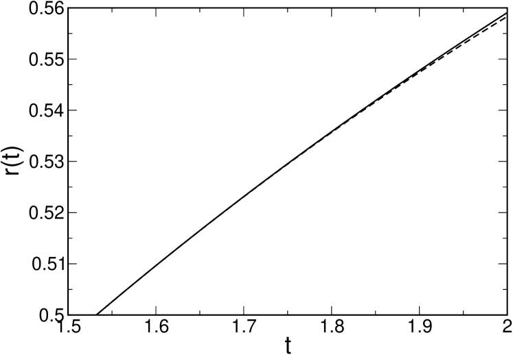
Figure 2: Shown are the paramagnetic (solid, $q=0$) and spin glass(dashed, $q>0$) solutions to Eq. (LABEL:13c). After the critical point at $r=1/2$, the spin glass phase relaxes more slowly than does the paramagnetic phase. Here $C=12$.

This calculation suggests that the energy relaxation is universal, i.e. $r(t)$ does not have an explicit dependence on the modularity, $M$. Presumably, this is because the effect of modularity is a finite size effect. It also happens that projecting the energy onto the $r_{I}$ and $r_{O}$ components gives the same result as projecting the energy onto $r$.

VI Finite-Size Corrections to the Dynamics

Finite-size scaling of spin glass thermodynamics near the phase transition has been analyzed by the TAP equations Bray and Moore (1979). The analysis proceeds by analyzing a matrix that at the transition has the form $A_{ij}=2I-J_{ij}$. The density of eigenvalues, $\lambda$, takes the form $\rho(\lambda)=\sqrt{\lambda}/\pi$ for small $\lambda$. The susceptibility goes as $\chi=\int d\lambda\rho(\lambda)/\lambda^{2}\sim 2\lambda_{1}^{-1/2}/\pi$ where $\lambda_{1}$ is the smallest eigenvalue. It has been argued that finite size thermodynamics for a spin glass of size $N$ can be understood by thermodynamics of an infinite spin glass with a finite value of $K$ in the Parisi RSB scheme Aspelmeier et al. (2008). It is argued that to stabilize the Gaussian propagator, the self-energy in the RSB scheme, $4\Delta t^{2}/(2K+1)^{2}/3$, with $\Delta t=1-T/T_{c}$, should be set to the inverse of the susceptibility, calculated above as $\pi\lambda_{1}^{1/2}/2$ Aspelmeier et al. (2008); Janis and Klic (2006). Corrections to the spin coupling parameter scale as $q=\Delta t+\Delta t^{2}-2\Delta t^{2}/(2K+1)^{2}/3$ Janis and Klic (2006). Combining these results, one finds

$$q=2\epsilon-\pi\lambda_{1}^{1/2}/4$$ (25)

The factor $\pi/4$ is only an estimate and may be replaced by another constant. For a Gaussian coupling matrix, $\lambda_{1}\sim N^{-2/3}$ Bray and Moore (1979), and $\lambda_{1}$ is distributed according to the Tracy-Widom distribution Tracy and Widom (1993), This distribution is universal for matrices with variances equal to the Gaussian ensemble and symmetric probability distributions Soshnikov (1999). We, thus, conclude

$$q = 2\epsilon-\Delta q,$$

$$\Delta q \approx \pi N^{-1/3}/4$$ (26)

Expression (26) tells us the finite size effects on $dr/dt$ for large $N$ for non-modular matrices, with $M=0$. For a perfectly modular matrix, $M=1$, we can use this expression with $N\to L$. In Appendix C, we show that $\lambda_{1}$ increases from the $M=0$ value to the $M=1$ value. Thus, $q$ will be somewhat smaller in the $M=1$ case than in the $M=0$ case. Near $r=1/2+\epsilon$ , for $C\to\infty$ and $q=O(\epsilon)$, the dynamical equation (LABEL:13c) takes the form

$$\frac{dr}{dt} = -2r+1.167+1.365\epsilon+0.968\epsilon^{2}-0.242q(M)^{2}+O(\epsilon^{3})$$ (27)

Since $q$ becomes smaller as $M$ increases from 0 to 1, we see that $r_{M}(t)>r_{M=0}(t)$ for $r>1/2$. Thus, this calculation suggests that modularity increases the rate of relaxation for $t>t_{c}$. Interestingly, if $q=2\epsilon$, a non-vanishing $q$ exactly cancels the $O(\epsilon^{2})$ term in the above expression.

VII Numerical Results

We here use a Lebowitz-Gilespie algorithm to sample the continuous-time Markov process that describes the Glauber dynamics that lead to Eq. LABEL:13c Bortz et al. (1975); Gillespie (1976); Coolen and Sherrington (1994). We first consider the case of a small matrix, $N=64$, with $k_{1}=4,C=16$. We performed $10^{6}$ samplings of the Markov process, collecting the continuous time $r(t)$ curves into bins in time. For large matrices and short times, $t\ll t_{c}$, the results reproduce those of Eq. (LABEL:13c), which are independent of $M$, in agreement with previous calculations for $M=0$ Laughton et al. (1996). The average results for small matrices with $M=0$ and $M=1$ are shown in Fig. 3. The response function of the modular matrix is below that of the non-modular matrix.

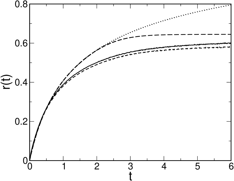
Figure 3: Shown is the $r(t)$ curve for $N=64,N/L=4,C=16$ for $M=0$ (solid) and $M=1$ (short dashed). Also shown is the prediction of Eq. (LABEL:13c) for $r^{\rm PARA}(t)$ (dotted) and $r^{\rm SG}(t)$ (long dashed).

We next consider the case of a large matrix, $N=16000$ with $k_{1}=4,C=4000$. This is a large matrix, so we performed $10^{3}$ samplings of the Markov process for $M=0$ and $M=1$. We performed the calculation independently two times, and the results are qualitatively similar, with a crossing of the average $r_{M=1}(t)$ and $r_{M=0}(t)$ curves at some $t>t_{c}$. We fit difference between the continuous time $r(t)$ curves for $t>t_{c}$ to $k^{\rm th}$ order polynomials in time, shown in Fig. 4. There is an interval after the critical point, $t_{c}<t<t^{*}$ during which the response function of the modular matrix appears to be above that of the non-modular matrix. The standard error of the average of the histogrammed points in this range is $5.1\times 10^{-5}$. Thus, the observed difference between the $M=1$ and $M=0$ response functions is about two standard errors. From equilibrium finite size effects, we know $r_{M=1}(t)-r_{M=0}(t)=\Delta r(t)<0$ for large enough $t$, and Fig. 4b reproduces this expected trend.

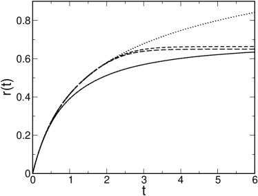
a) b)

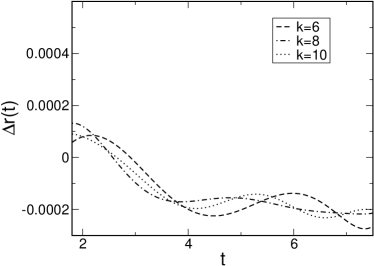
Figure 4: a) The $8^{\rm th}$ order polynomial fits to $r(t)$ for $N=16000,N/L=4,C=4000$ for $M=0,1$. The $M=0$ and $M=1$ curves (solid) are indistinguishable on this scale. Also shown is the prediction of Eq. (LABEL:13c) for $r^{\rm PARA}(t)$ (dotted), $r^{\rm SG}(t)$ (long dashed), and $r^{\rm SG}(t)$ using Eq. (26) (short dashed). b) Shown is the $k^{\rm th}$ order polynomials curve fits for $k=6,8,10$ to the difference, $r_{M=1}(t)-r_{M=0}(t)$, between 2000 samples of the Markov process.

The projection of the dynamics to $r_{I},r_{O},m$ in Eq. (2) is approximate. A more accurate approximation is obtained by projecting to the distribution of local fields Laughton et al. (1996). The result is qualitatively similar to Fig. 4a: the spin glass phase emerges at $t_{c}$ when $q>0$, and $r^{\rm SG}(t)<r^{\rm PARA}(t)$. Quantitatively, $t_{c}$ shifts from 1.439 for $C\to\infty$ to a value $1.85$, also observed in the numerical simulations here. We expect that the argument of Eq. (26) will also apply to this more involved calculation, which again, does not take into account the $t\to\infty$ finite size effects. We expect that the qualitative conclusions for such a calculation will be similar to those of Section VI.

VIII Discussion

For Glauber dynamics, the effect of modularity on the dynamics at short time is a small finite-size effect. From Figure 2 we see that the difference between the paramagnetic and spin glass dynamics is not large near $t_{c}$, and the effects of modularity are only a small perturbation of the spin glass dynamics, Eq. (26). At long time, there is a clear effect of modularity, because the less modular matrix converges to a more stable energy per spin than does a more modular matrix. Figure 4b suggests a modest crossing of the $r_{M=1}(t)$ and $r_{M=0}(t)$ curves after $t_{c}$.

The results of Fig. 4 are not dramatic and are smaller than Eqs. (LABEL:13c) and (26) would predict. Eq. (26) is approximate and cannot be used near $r=1/2$, but if it is, it predicts an effect $10\times$ larger than what is observed in Fig. 4 at $t=t_{c}+0.4$. What Eqs. (LABEL:13c) and (26) miss is the equilibrium finite size effects for large $t$. These effects are opposite in sign to what Eq. (26) suggests and cause $r_{M}(t)<r_{M=0}(t)$ for large enough $t$.

In biology horizontal gene transfer significantly enhances the emergence of modularity in different individuals evolving on a common, rugged fitness landscape Sun and Deem (2007). In the spin glass language, the simple mechanistic picture is that different instances of the dynamical ensemble can find states that approximately optimize $r$ within one of the $L\times L$ block diagonals. Horizontal gene transfer can then combine $N/L$ of these partial solutions of length $L$ into a near optimal state of length $N$. This recombination of partial states is thought to exponentially speed up identification of optimal states. Due to the mean field nature of model (1), nucleation of correlations corresponding to ground states in the modules is averaged out. Perhaps more significantly, the Glauber dynamics studied here does not have the multi-spin flip analog of the horizontal gene transfer move.

IX Conclusion

We have performed a replica calculation for the dynamics of a dilute, modular SK model. Correlations in this model were defined by a connection matrix, which was parametrized by its modularity. These calculations suggest that the energy relaxation of the dilute SK model is universal, independent of the value of modularity for infinite systems. Finite size arguments show that a non-modular matrix relaxes to a more stable energy at long times. Finite size arguments suggest that the energy relaxation may be quicker for a modular connection matrix, possibly leading to more slightly favorable energy values at intermediate times near the spin glass transition. The effect for Glauber dynamics is quite modest.

Interestingly, in biology horizontal gene transfer significantly enhances the emergence of modularity, and modularity can enhance biological fitness Sun and Deem (2007). In the absence of horizontal gene transfer, modularity does not significantly change fitness in these models. The present statistical mechanics calculations, showing little dynamic effect of modularity, are consistent with the latter biological results. The Glauber dynamics used here do not contain a multi-spin move that is analogous to horizontal gene transfer. Calculation of the effect of horizontal gene transfer for finite, modular biological systems is an open problem.

X Appendix A: Stability of the Overlap function

We expand Eq. (23) to second order in $q_{I}$ and $q_{O}$, using Eq. (21) and replica symmetry. This coupled set of equations can be solved by the quartic formula to yield four solutions, with lengthy explicit expressions. The first solution is $q_{I}^{A}=q_{O}^{A}=0$. The second solution can be found by setting $q_{I}^{B}=q_{O}^{B}=q^{B}$, with solution $q^{B}=(4r^{2}-1)/(32r^{4})$. The third solution can be found by searching for a solution that goes to zero at $r_{0}^{C}$ and is of order $r-r_{0}^{C}$. This yields an additional solution with $q_{I}^{C}\neq q_{O}^{C}$ and $r_{0}^{C}=1/(2\sqrt{M})$. Near $r_{0}$, this solution looks like $q_{I}^{C}=-(k_{1}-1)q_{O}^{C}=2(k_{1}-1)/(k_{1}-2)\sqrt{M}(r-r_{0}^{C})$. There is a fourth solution that changes from complex to real at $r_{0}^{D}=[1+2(1-M)\sqrt{k_{1}-1}/(k_{1}M)]^{1/2}/2$. Interestingly $q^{C}$ also turns from complex to real at $r_{0}^{D}$, with $q_{I}^{C}(r_{0}^{D})=q_{I}^{D}(r_{0}^{D})$ and $q_{O}^{C}(r_{0}^{D})=q_{O}^{D}(r_{0}^{D})$.

The solution that is most stable is the one which extremizes (which means maximize as $n\to 0$) the dynamical free energy. The dynamical free energy is

$$\beta\overline{f} = -\lim_{n\to 0}f^{*}/n$$ (28)

$$= -\ln 2+\frac{\rho_{I}^{2}}{4a}+\frac{\rho_{O}^{2}}{4b}-\frac{3}{4}\frac{\rho_{I}^{2}}{a}\left(\frac{1}{k_{1}}q_{I}^{2}+\frac{k_{1}-1}{k_{1}}q_{O}^{2}\right)-\frac{3}{4}\frac{\rho_{O}^{2}}{b}\left(\frac{2}{k_{1}}q_{I}q_{O}+\frac{k_{1}-2}{k_{1}}q_{O}^{2}\right)$$

$$+\frac{1}{4k_{1}}\left(\frac{\rho_{I}^{2}q_{I}}{a}+\frac{\rho_{O}^{2}q_{O}}{b}\right)^{2}+\frac{k_{1}-1}{4k_{1}}\left(\frac{\rho_{I}^{2}q_{O}}{a}+\frac{\rho_{O}^{2}(q_{I}+(k_{1}-1)q_{O}}{k_{1}b}\right)^{2}$$

The dynamical free energy can be evaluated for the four solutions. We consider $g=\beta\bar{f}+\ln 2$. We find $g^{A}=r^{2}$. When $q_{I}=q_{O}$, we find $g=r^{2}+\epsilon q_{I}^{2}$, so that $g^{B}=r^{2}+4\epsilon^{3}$. At $r_{0}^{D}$, we find $g^{C}=g^{D}=r^{2}-4\epsilon^{3}[k_{1}^{2}-4k_{1}(\sqrt{k_{1}-1}-1)-4]/(8k_{1}\sqrt{k_{1}-1})$. The term proportional to $\epsilon^{3}$ in $g^{C}=g^{D}$ is always negative, so that solution B is more stable at $r_{0}^{D}$. At $r_{0}^{C}$, $g^{C}=r^{2}$. We find that $g^{D}(r_{0}^{C})={r_{0}^{C}}^{2}+4\epsilon^{3}[1-8/k_{1}+24/k_{1}^{2}-32/k_{1}^{3}-16/k_{1}^{4}]$. For $k_{1}>1$, solution B is again most stable. There does not appear to be a crossing of the C,D free energies with the more stable B free energy. We, thus, find solution B is most stable for $r>1/2$.

XI Appendix B: $dr_{I}/dt$ and $dr_{O}/dt$

At the saddle point, Eq. (16) becomes

$$D_{m,r_{I},r_{O}}[x,y]=\lim_{N\to\infty}\lim_{n\to 0}\int\frac{d\xi d\eta}{(2\pi)^{2}}e^{i\xi x+i\eta y}\frac{{\rm Tr}_{\sigma}e^{g(\sigma)+X_{I}(\sigma)}}{{\rm Tr}_{\sigma}e^{X_{I}(\sigma)}}$$ (29)

since $f^{*}=-\beta n\bar{f}\to 0$. Here $g(\sigma)=g_{1}(\xi,\rho_{I},q_{I})/a+g_{1}(\eta,\rho_{O},q_{O})/b$ where

$$g_{1}(x,\rho,q) = C(e^{-x^{2}/(2C)}-1)-ix\rho e^{-x^{2}/(2C)}\sigma_{1}-ix\rho e^{-x^{2}/(2C)}\sum_{1<\alpha}q_{1\alpha}\sigma_{\alpha}$$ (30)

$$+\rho^{2}(1-x^{2}/C)e^{-x^{2}/(2C)}\sum_{\alpha<\beta}q_{\alpha\beta}\sigma_{\alpha}\sigma_{\beta}$$

We also have

$$X_{I}(\sigma)=\sum_{\alpha<\beta}\left[\frac{\rho_{I}^{2}q_{\alpha\beta}^{I}}{a}+\frac{\rho_{O}^{2}q_{\alpha\beta}^{O}}{b}\right]\sigma_{\alpha}\sigma_{\beta}$$ (31)

Near the spin glass transition, the $q$ are small. Assuming replica symmetry, we find

$${\rm Tr}_{\sigma}e^{X_{I}(\sigma)}=1+n(n-1)(\rho_{I}^{2}q^{I}/a+\rho_{O}^{2}q_{O}/b)^{2}/4+O(q^{3})\to 1{\rm~{}as~{}}n\to 0$$ (32)

We also find

$${\rm Tr}_{\sigma}e^{g(\sigma)+X_{I}(\sigma)} = e^{C(e^{-\xi^{2}/(2C)}-1)/a+C(e^{-\eta^{2}/(2C)}-1)/b}{\rm Tr}_{\sigma}e^{f_{1}\sigma_{1}+\sum_{1<\alpha}f_{\alpha}\sigma_{\alpha}+\sum_{\alpha<\beta}F_{\alpha\beta}\sigma_{\alpha}\sigma_{\beta}}$$ (33)

where

$$f_{1} = -i\xi\rho_{I}e^{-\xi^{2}/(2C)}/a-i\eta\rho_{O}e^{-\eta^{2}/(2C)}/b$$

$$f_{\alpha} = -i\xi\rho_{I}e^{-\xi^{2}/(2C)}q_{1\alpha}^{I}/a-i\eta\rho_{O}e^{-\eta^{2}/(2C)}q_{1\alpha}^{O}/b$$

$$F_{\alpha\beta} = \rho_{I}^{2}(1-\xi^{2}/C)e^{-\xi^{2}/(2C)}q_{\alpha\beta}^{I}/a+\rho_{O}^{2}(1-\eta^{2}/C)e^{-\eta^{2}/(2C)}q_{\alpha\beta}^{O}/b$$ (34)

Taking the trace over $\sigma_{\alpha>1}$, we find

$${\rm Tr}_{\sigma}e^{g(\sigma)+X_{I}(\sigma)} = e^{C(e^{-\xi^{2}/(2C)}-1)/a+C(e^{-\eta^{2}/(2C)}-1)/b}$$ (35)

$$\times{\rm Tr}_{\sigma_{1}}e^{f_{1}\sigma_{1}}\left[1+\frac{1}{2}(n-1)f^{2}+(n-1)fF\sigma_{1}+\frac{(n-1)(n-2)}{2}F^{2}+(n-1)F^{2}\right]$$

$$\to e^{C(e^{-\xi^{2}/(2C)}-1)/a+C(e^{-\eta^{2}/(2C)}-1)/b}\left[\left(1-\frac{f^{2}}{2}\right)\cosh f_{1}-fF\sinh f_{1}\right]{\rm~{}as~{}}n\to 0$$

$$\equiv G(\xi,\eta)$$

We consider the dynamical equations (2) in the limit $\beta J\to\infty$, so that $\tanh\beta J(x+y)\to{\rm sgn}(x+y)$. We can integrate out the $x,y$ dependence in Eq. (2) given Eq. (29) by using integration by parts to see

$$\int dxdye^{i\xi x+i\eta y}x{\rm sgn}(x+y)=2(2\pi)\frac{\delta^{\prime}(\xi-\eta)}{\eta}$$ (36)

and

$$\int dxdye^{i\xi x+i\eta y}y{\rm sgn}(x+y)=2(2\pi)\frac{\delta^{\prime}(\eta-\xi)}{\xi}$$ (37)

Eq. (2) and integration by parts leads to

$$\frac{dr_{I}}{dt} = -2r_{I}-\frac{1}{\pi}{\rm Re}\int_{-\infty}^{\infty}\frac{d\eta}{\eta}\left[\frac{d}{d\xi}G(\xi,\eta)\right]_{\xi=\eta}$$

$$\frac{dr_{O}}{dt} = -2r_{O}-\frac{1}{\pi}{\rm Re}\int_{-\infty}^{\infty}\frac{d\xi}{\xi}\left[\frac{d}{d\eta}G(\xi,\eta)\right]_{\eta=\xi}$$ (38)

Evaluating these derivatives, we find

$$\frac{dr_{I}}{dt} = \frac{1}{a}\frac{dr}{dt}$$

$$\frac{dr_{O}}{dt} = \frac{1}{b}\frac{dr}{dt}$$ (39)

where

$$\frac{dr}{dt} = -2r-\frac{1}{\pi}{\rm Re}\int_{-\infty}^{\infty}\frac{d\eta}{\eta}\frac{d}{d\eta}\bigg{\{}e^{-C+Ce^{-\eta^{2}/(2C)}+i\eta(\rho_{I}/a+\rho_{O}/b)e^{-\eta^{2}/(2C)}}$$ (40)

$$\bigg{[}1+\frac{1}{2}\left(\frac{\rho_{I}q_{I}}{a}+\frac{\rho_{O}q_{O}}{b}\right)^{2}\eta^{2}e^{-\eta^{2}/C}$$

$$-i\left(\frac{\rho_{I}q_{I}}{a}+\frac{\rho_{O}q_{O}}{b}\right)\left(\frac{\rho_{I}^{2}q_{I}}{a}+\frac{\rho_{O}^{2}q_{O}}{b}\right)\eta(1-\eta^{2}/C)e^{-\eta^{2}/C}\bigg{]}\bigg{\}}$$

Using Eq. (21) and replica symmetry leads to Eq. (LABEL:13c).

XII Appendix C: Distribution of smallest eigenvalue for a modular matrix

We here consider how the smallest eigenvalue of a modular matrix changes from the $N^{-1/3}$ scaling to the $L^{-1/3}$ scaling as $M$ increases from 0 to 1 in a random modular matrix. Up to logarithmic corrections, the density of states and the distribution of the smallest eigenvalue of any large random matrix are equivalent to that of a large matrix from the Gaussian ensemble, essentially as long as $\langle J_{ij}\rangle^{2}$, which may depend on $i$ and $j$, is the same in the two cases Erdös and Yau (2012). We, therefore, consider the matrix

$$B(M)=2I+\sqrt{M}A_{1}+\sqrt{1-M}A_{0}$$ (41)

where $A_{1}$ is a block diagonal symmetric random Gaussian matrix with variance $1/L$ in the $L\times L$ blocks and $A_{0}$ is a $N\times N$ symmetric random Gaussian matrix with variance $1/N$ at all entries. For any $M$, the sum of the variances of in a row is unity. We consider the standard deviation of the smallest eigenvalue of this matrix, $\sigma_{M}(\lambda_{1})$. We expect $\sigma_{M}/\sigma_{0}$ goes from 1 to $d(N/L)^{2/3}$ as $M$ increases from 0 to 1, where $d$ is the standard deviation of the maximum of $N/L$ Tracy-Widom random variables divided by the standard deviation of one Tracy-Widom random variable. The form of this function is shown in Figure 5 for the case $N/L=4$. We see that $\sigma_{M}/\sigma_{0}$ increases with $M$. Whether there is spectral rigidity for $M<M^{*}$ in the limit $N\to\infty$ is unclear Erdös et al. (2013). Recall that $\sigma_{M}/\sigma_{0}>1$ implies the response curve in Figure 2 in the spin glass phase lies above the curve for $M=0$.

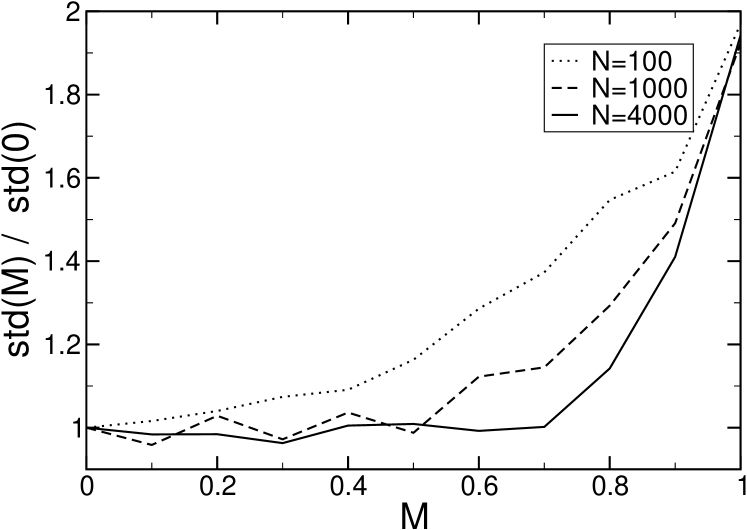
Figure 5: Shown is standard deviation of the smallest eigenvalue of the matrix defined by Eq. (41) as a function of modularity. Here $N/L=4$.

References

He et al. (2009)
J. He,
J. Sun, and
M. W. Deem,
Phys. Rev. E 79,
031907 (2009).
Lorenz et al. (2011)
D. Lorenz,
A. Jeng, and
M. W. Deem,
Phys. Life Rev. 8,
129 (2011).
Clune et al. (2013)
J. Clune,
J.-B. Mouret,
and H. Lipson,
Proc. Roy. Soc. B 280,
20122863 (2013).
Friedlander et al. (2013)
T. Friedlander,
A. E. Mayo,
T. Tlusty, and
U. Alon,
PLoS ONE 8,
e70444 (2013).
Anderson (1983)
P. W. Anderson,
Proc. Natl. Acad. Sci. USA 80,
3386 (1983).
Kauffman and Levin (1987)
S. Kauffman and
S. Levin, J.
Theor. Biol. 128, 11
(1987).
Sakata et al. (2009)
A. Sakata,
K. Hukushima,
and K. Kaneko,
Phys. Rev. Lett. 102,
148101 (2009).
Sakata et al. (2012)
A. Sakata,
K. Hukushima,
and K. Kaneko,
Euro. Phys. Lett. 99,
68004 (2012).
Pradhan et al. (2011)
N. Pradhan,
S. Dasgupta, and
S. Sinha,
Eur. Phys. Lett. 94,
38004 (2011).
Breen et al. (2012)
M. S. Breen
et al., Nature
490, 535 (2012).
Bogarad and Deem (1999)
L. D. Bogarad and
M. W. Deem,
Proc. Natl. Acad. Sci. USA 96,
2591 (1999).
Sun et al. (2005a)
J. Sun,
D. J. Earl, and
M. W. deem,
Phys. Rev. Lett. 95,
148104 (2005a).
Sun et al. (2006)
J. Sun,
D. J. Earl, and
M. W. deem,
Mod. Phys. Lett. B 20,
63 (2006).
Khatri et al. (2009)
B. S. Khatri,
T. C. McLeish,
and R. P. Sear,
Proc. Natl. Acad. Sci. USA
1006, 9564
(2009).
Vetsigian et al. (2006)
K. Vetsigian,
C. Woese, and
N. Goldenfeld,
Proc. Natl. Acad. Sci. USA 103,
10696 (2006).
Deem and Lee (2003)
M. W. Deem and
H. Y. Lee,
Phys. Rev. Lett. 91,
068101 (2003).
Park and Deem (2004)
J.-M. Park and
M. W. Deem,
Physica A 341,
455 (2004).
Sun et al. (2005b)
J. Sun,
D. J. Earl, and
M. W. Deem,
Proc. Natl. Acad. Sci. USA 95,
148104 (2005b).
Zhou and Deem (2006)
H. Zhou and
M. W. Deem,
Vaccine 24,
2451 (2006).
Gupta et al. (2006)
V. Gupta,
D. J. Earl, and
M. W. Deem,
Vaccine 24,
3881 (2006).
Yang et al. (2006)
M. Yang,
J.-M. Park, and
M. W. Deem,
Physica A 366,
347 (2006).
Pan and Deem (2011)
K. Pan and
M. W. Deem,
Phys. Biol. 8,
055006 (2011).
G. Parisi and Slanina (1993a)
F. R. G. Parisi
and F. Slanina,
J. Phys. A 26,
247 (1993a).
G. Parisi and Slanina (1993b)
F. R. G. Parisi
and F. Slanina,
J. Phys. A 26,
3775 (1993b).
Billoire (2006)
A. Billoire,
Phys. Rev. B 73,
132201 (2006).
Aspelmeier et al. (2008)
T. Aspelmeier,
A. Billoire,
E. Marinari, and
M. A. Moore,
J. Phys. A: Math. Gen. 41,
324008 (2008).
Bouchaud et al. (1998)
J.-P. Bouchaud,
L. F. Cugliandolo,
J. Kurchan, and
M. Mézard, in
Spin Glasses and Random Fields, edited by
A. P. Young
(World Scientific, 1998),
vol. 12, pp. 161–224.
Kinzelbach and Horner (1991)
H. Kinzelbach and
H. Horner,
Z. Phys. B—Cond. Matt. 84,
95 (1991).
Bittner et al. (2008)
E. Bittner,
A. Nubaumer,
and W. Janke, in
NIC Symposium, edited by
G. Münster,
D. Wolf, and
M. Kremer
(John von Neumann Institute for Computing,
2008), vol. 39, pp.
229–236.
Dotsenko (1985)
V. S. Dotsenko,
J. Phys. C: Solid State Phys.
18, 6023 (1985).
Waddington (1942)
C. H. Waddington,
Nature 150,
563 (1942).
Simon (1962)
H. A. Simon,
Proc. Amer. Phil. Soc. 106,
467 (1962).
Hartwell et al. (1999)
L. H. Hartwell,
J. J. Hopfield,
S. Leibler, and
A. W. Murray,
Nature 402,
C47 (1999).
Kashtan et al. (2009)
N. Kashtan,
M. Parter,
E. Dekel,
A. E. Mayo, and
U. Alon,
Evolution 63,
1964 (2009).
Wagner et al. (2007)
G. P. Wagner,
M. Pavlicev, and
J. M. Cheverud,
Nat. Rev. Genet. 8,
921 (2007).
Sun and Deem (2007)
J. Sun and
M. W. Deem,
Phys. Rev. Lett. 99,
228107 (2007).
Kinzel (1986)
W. Kinzel,
Phys. Rev. B 33,
5086 (1986).
Coolen and Sherrington (1994)
A. C. C. Coolen
and
D. Sherrington,
J. Phys. A: Math. Gen. 27,
7687 (1994).
Bray and Moore (1979)
A. J. Bray and
M. A. Moore,
J. Phys. C: Solid State Phys.
12, L441 (1979).
Janis and Klic (2006)
V. Janis and
A. Klic,
Phys. Rev. B 74,
054410 (2006).
Tracy and Widom (1993)
C. A. Tracy and
H. Widom,
Phys. Lett. B 305,
115 (1993).
Soshnikov (1999)
A. Soshnikov,
Comm. Math. Phys 207,
697 (1999).
Bortz et al. (1975)
A. B. Bortz,
M. H. Kalos, and
J. L. Lebowitz,
J. Comput. Phys. 17,
10 (1975).
Gillespie (1976)
D. T. Gillespie,
J. Comput. Phys. 22,
403 (1976).
Laughton et al. (1996)
S. N. Laughton,
A. C. C. Coolen,
and
D. Sherrington,
J. Phys. A: Math. Gen. 29,
763 (1996).
Erdös and Yau (2012)
L. Erdös and
H.-T. Yau,
Bull. Amer. Math. Soc. 49,
377 (2012).
Erdös et al. (2013)
L. Erdös,
A. Knowles,
H.-T. Yau, and
J. Yin,
Electron. J. Probab. 18,
1 (2013).
b)
b)