Phase Description of Stochastic Oscillations

Abstract

We introduce an invariant phase description of stochastic oscillations by generalizing the concept of standard isophases. The average isophases are constructed as sections in the state space, having a constant mean first return time. The approach allows to obtain a global phase variable of noisy oscillations, even in the cases where the phase is ill-defined in the deterministic limit. A simple numerical method for finding the isophases is illustrated for noise-induced switching between two coexisting limit cycles, and for noise-induced oscillation in an excitable system. We also discuss how to determine the isophases for experimentally observed irregular oscillations, providing a basis for a refined phase description of observed oscillatory dynamics.

Phase reduction is the basic tool in the characterization of self-sustained, autonomous oscillators. With a reasonably defined phase variable, one obtains a one-dimensional representation of the oscillator, allowing to describe important aspects of its dynamics, such as regularity, sensitivity to forcing and noise, etc Winfree (1980); Kuramoto (1984); Pikovsky et al. (2001). Furthermore, the concept of phase reduction is substantial for the data analysis of oscillatory processes in physics, chemistry, biology, and technical applications, where various approaches exist for extracting phases from oscillatory time series Schäfer et al. (1998); Rosenblum and Pikovsky (2001); Tokuda et al. (2007); Bartsch et al. (2007); Stankovski et al. (2012).

To understand many properties of oscillating systems, such as their phase resetting and synchronizability, it is important to define the phases not only for the purely periodic motion, but for the whole state space. In the theory of deterministic oscillations this is done via so-called isochrones Guckenheimer (1975), by attributing to a state with an arbitrary amplitude the phase of a point on the limit cycle, to which this state asymptotically converges. In this letter we generalize this concept to irregular, noisy oscillators. The main idea is based on the definition of the isophases by virtue of the mean first passage time concept. We will first apply our method to noise-perturbed deterministic oscillators for which the isophases can be compared with deterministic isochrones. Furthermore, we will consider examples for which the isochrones and even the oscillations themselves disappear in the deterministic limit. The method will be also applied to noise-perturbed chaotic oscillations. Finally, we will demonstrate its applicability to experimentally observed time series.

We start by reminding the standard definition of isophases (which in this case are also isochrones) in deterministic systems with a stable limit cycle $\mathbf{x}_{0}(t)=\mathbf{x}_{0}(t+T)$ having period $T$. First, one defines the phase on the limit cycle $\varphi(\mathbf{x}_{0})$. Then, being observed stroboscopically with time interval $T$, all the points $\mathbf{x}$ that converge to a particular point on the cycle $\mathbf{x}_{0}$ having the phase $\varphi(\mathbf{x}_{0})$. These points form a Poincaré surface of section $J(\varphi(\mathbf{x}_{0}))$ for the trajectories of the dynamical system, with the special property that the return time to this surface equals $T$ for all points on it. Thus, to find an isophase surface is equivalent to find a Poincaré surface of section with the constant return time $T$.

For a noisy system we define the isophase surface $J$ as a Poincaré surface of section, for which the mean first return time $J\to J$, after performing one full oscillation, is a constant $T$, having a meaning of the average oscillation period. In order for isophases to be well-defined, oscillations have to be well-defined as well: amplitudes should always remain positive (so that one can reliably recognize a “full oscillation”). Otherwise the concept of phase is not well-defined for a random process, and the isophases are not meaningful.

Analytical calculations of the mean first return time (MFRT) is a complex problem in dimensions larger than one, therefore below we apply a simple numerical algorithm for construction of the isophases: an initial Poincaré section is iteratively altered until all mean return times are approximately equal. In two-dimensional systems for which isophases are lines, we represent Poincaré sections by a linear interpolation in between a set of knots. For each knot $x_{j}$, the average return time $T_{j}$ is computed via the Monte Carlo simulation. According to the mismatch of $T_{j}$ and the mean period $\langle T\rangle$, the knot $x_{j}$ is advanced or retarded. The procedure is repeated with all knots, until it converges and all return times $T_{j}$ are nearly equal to $\langle T\rangle$.

Before proceeding to different applications of this procedure, we discuss the importance of knowing isophases for noisy oscillations. The first important application is that of phase resetting. Phase resetting curve determines how an oscillator responds to an external kick, this response determines synchronization properties of oscillator Ermentrout and Saunders (2006); Achuthan and Canavier (2009). For deterministic oscillators the phase response curve is determined just from the isochrone to which the kick shifts the state of the system from the limit cycle. For irregular oscillators the proper definition of the phase response curve is based on the first passage time Schwabedal and Pikovsky (2010), so to determine it one has to find to which isophase, as defined above, the system is shifted by the kick (note that in the limit of small noise, perturbative approaches for the phase dynamics do the job Teramae et al. (2009); Goldobin et al. (2010)). The second application is in the analysis of experimental data of coupled oscillators (cf. Schäfer et al. (1998); Rosenblum and Pikovsky (2001); Tokuda et al. (2007); Bartsch et al. (2007); Stankovski et al. (2012)). There one needs to determine the phase dynamics from the time series, this task is relatively simple to accomplish if the variations of the amplitudes are very small so that the definition of a phase-like variable along the observed limit cycle is unambiguous. However, in the presence of large irregular amplitude variations, the phase characterization of the oscillations is not unique (cf. Fig. 6 below). Proceeding according to the given above definition of the isophases as the lines on the two-dimensional embedding plane, for which the mean return times do not depend on the amplitudes, allows us to get rid of the ambiguity and to determine the phase in a consistent way.

We stress here that in our definition of the isophases we do not assume Markovian property of the process, if the dynamics is non-Markovian, then the definition of the MFRT includes averaging over the “prehistory” or hidden variables as well. To illustrate this we consider as the first example a simple Stuart-Landau oscillator (variables $r,\theta$) perturbed by an Ornstein-Uhlenbeck noise (OUN) $\zeta(t)$:

$$\dot{r} =r(1-r^{2})+\sigma r\zeta(t)\;,\qquad\dot{\theta}=\omega-\kappa(r^{2}-1),$$ (1)

$$\gamma\dot{\zeta} =-\zeta+\sqrt{\gamma}\xi(t)~{},$$

where $\xi(t)$ denotes a $\delta$-correlated white noise, $\gamma$ is the correlation time of the OUN, $\omega$ is the frequency of the noise-free limit cycle, and $\kappa$ is a nonisochronicity parameter. In the state space $r,\theta,\zeta$ the process is Markovian, but on the two-dimensional plane $r,\theta$ it is not. Nevertheless, by the method described we obtain numerical isophase for which the MFRT is nearly constant (Fig. 1). This isophase can be obtained also from the following analytic approximation. First, we introduce a “corrected” phase variable $\psi=\theta-\kappa\ln r$ which obeys $\dot{\psi}=\omega+\sigma\kappa(\gamma\dot{\zeta}-\sqrt{\gamma}\xi(t))$. Averaging this expression and identifying $\omega=\dot{\varphi}$ where $\varphi$ is the correct uniformly rotating phase, we obtain $\varphi=\psi-\sigma\kappa\gamma\zeta$. In this expression we have to account for correlations of $\zeta$ and $r$, to obtain the isophases on the plane $(\theta,r)$. Assuming that $r$ follows $\zeta(t)$ adiabatically, we obtain $\sigma\zeta\approx r^{2}-1$, what leads to the following expression for the isophases

$$\varphi=\theta-\kappa\ln r-\kappa\gamma\left(r^{2}-1\right)~{}.$$ (2)

Isophase following from this formula is compared with numerical one in Fig. 1. Interestingly, the noise-induced correction (last term in (2)) does not contain parameter $\sigma$, but the range where this correction is valid $|r-1|\lesssim\sigma$ shrinks with the noise amplitude.

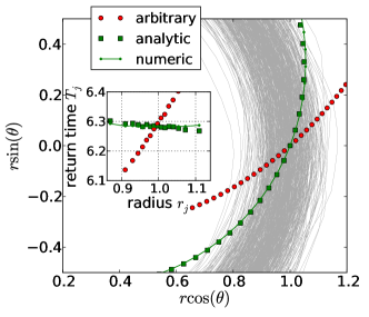
Figure 1: (color online) The average isophase for noise-driven oscillator [Eq. 1] with $\omega=1,\kappa=1,\sigma=0.15,\gamma=1$ in cartesian coordinates. The inset shows the reduction of the variations of the MFRT compared to an arbitrary cross-section. The numerically-derived isophase shows minor differences to the analytic approximation [Eq. 2].

While in the simplest example above the effect of noise is in the correction of the deterministic isochrones only, we consider now a situation where local isophases of different periodic motions are “mixed” by noise resulting in new, global isophases. To this end we analyze the following model of two coexisting stable limit cycles, driven by white noise:

$$\dot{r} =r(1-r)(3-r)(c-r)+\sigma\xi(t)~{},$$ (3)

$$\dot{\theta} =\omega+\delta(r-2)-(1-r)(3-r)~{}.$$

Without noise, the system shows two limit cycles $r_{I}=1,r_{II}=3$ (which have the same frequency if $\delta=0$), separated by an unstable cycle at $r=c$. Each of the stable cycles has its own isophases, which meet singularly (as infinitely rotating spirals) at the basin boundary $r=c$. With noise, trajectory switches between the basins, so that combined mixed-mode oscillations involving both cycles occur. By applying our method, we find the isophases of these oscillations in the whole range of the amplitudes, as shown in Fig. 2. While for small noise amplitude a residue of the singularity at the basin boundary is clearly seen, for a strong noise the isophases are rather smooth curves.

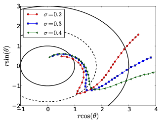
Figure 2: (color online) Isophases of bistable oscillations mixed by noise, in model (3) with $\omega=3,c=1.8,\delta=0$ and different noise intensities. Solid red curves are stable cycles, the dashed curve is the unstable cycle representing the basin boundary.

Another example where otherwise singular isophases are smeared by noise is that of chaotic oscillations. Many chaotic attractors allow a representation in terms of amplitudes and phases Farmer (1981); Pikovsky (1985); Pikovsky et al. (2001), but because the phase generally performs a chaos-induced diffusion, isophases in the strict sense do not exist. Recently, description of chaotic oscillations in terms of approximate isophases has been suggested Schwabedal et al. (2012). With noise, the return times to a Poincaré surface of a strange attractor can be defined in the averaged sense only, and in this respect there is no difference between chaotic and regular deterministic oscillators. Thus, the procedure of finding isophases based on the constancy of the MFRTs can be applied to chaotic systems as well, as is illustrated in Fig. 3 for the Roessler model

$$\dot{x} =-y-z+\sigma\xi_{1}(t)~{},$$ (4)

$$\dot{y} =x+0.16y+\sigma\xi_{2}(t)~{},$$

$$\dot{z} =0.2+z(x-10)~{},$$

with uncorrelated Gaussian white noises in $x$ and $y$ components.

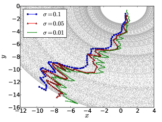
Figure 3: (color online) Isophases of the noise-driven Roessler chaotic system (4), for different noise intensities $\sigma$. Smaller noise leads to less smooth curves. Grey dots show the deterministic Roessler attractor.

Our final example are noise-induced oscillations in an excitable system, which without noise has just a stable steady state, so deterministic isophases do not exist in any sense. With noise, such a system demonstrates oscillations which may be quite regular in the case of coherence resonance Pikovsky and Kurths (1997). To build the model, we modify the noisy Stuart-Landau oscillator, with $y$- polarized noise, to perform noise-induced oscillations:

$$\dot{r} =r(1-r^{2})+\sigma r\cos\theta~{}\xi(t)~{},$$ (5)

$$\dot{\theta} =\omega+r\cos\theta-\kappa r^{2}+\sigma\sin\theta~{}\xi(t)~{}.$$

For $0<\omega-\kappa<1$ there is a stable state at $r_{0}=1,\theta_{0}=\pi-\arccos(\omega-\kappa)$ and an unstable state at $r_{1}=1,\theta_{1}=\pi+\arccos(\omega-\kappa)$ (at $\omega-\kappa=1$ they give rise to a periodic oscillation via a SNIPER bifurcation). Noise ($\sigma\neq 0$) excites the state $r_{0},\theta_{0}$ beyond $r_{1},\theta_{1}$ and produces noise-induced oscillations (Fig. 4). For strong excitability and small noise, the phase is well- defined, and the isophases can be introduced as curves with constant MFRTs. We show ten isophases in Fig. 5 (examples Fig. 1 and Fig. 2 have been rotationally symmetric, so one drawing of one isophase was sufficient, here the rotational symmetry is broken). The effect of the noise intensity on the isophases is maximal at $\theta\approx\pi$, i.e. in the region of excitability where the oscillations spend most of the time; in the “deterministic” region $|\theta|<\pi/2$ the isochrones are less sensitive to noise.

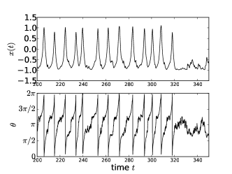
Figure 4: At $\omega=1.99$, $\kappa=1$, and $\sigma=0.6$, system (5) shows seemingly self-sustained oscillations (with some rather noisy patches as well), where indeed oscillations are noise-induced. Top panel: variable $x(t)=r\cos\theta$, bottom panel: $\theta(t)$.

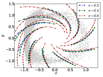
Figure 5: (color online). Average isophases of Eq. (5) at $\omega=1.99$ and $\kappa=1$ vary with noise intensity $\sigma$ as indicated. Larger noise intensity makes the system less isochronous, letting average isophases show stronger curvature. (Background trajectory of noise-induced oscillations (grey line) corresponds to the strong noise case $\sigma=0.6$.)

A practical definition of the isophases for which the MFRT is constant, is straightforward for numerical models of irregular oscillators as illustrated above, but it can be used for experimentally observed signals as well. For this purpose one needs a two-dimensional embedding of observed oscillations, which can be, e.g., achieved by using the Hilbert transform of the signal as the second variable. In Fig. 6 we present such a representation of measurements of human respiration, taken from the Physionet database . One can see that the oscillations have a large amplitude variability, and defining the phase has a large degree of ambiguity – contrary to the situations with a nearly constant amplitude, where a similar embedding on the signal vs its Hilbert transform plane results in a very narrow band of trajectories. The initial phase-like variables and the isophases resulting from the iterative procedure as described above are presented in Fig. 6. Application of the calculated isophases to determining the phase dynamics of the observed signals gives the mostly uniformly rotating phase, maximally uncorrelated from the amplitude variations.

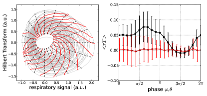
Figure 6: (color online). Left panel: Arbitrary phaselike variables (black) and isophases (red) of the experimental data of a respiration signal taken from the public database “Physionet”. Right panel: for isophases the return times are independent of the radial variable (cross-correlation vanishes).

Summarizing, we have introduced for irregular oscillations a concept of average isophases, based on the constancy of the mean first return times. By applying a simple procedure, we determined these isophases in a unified way for different classes of noisy oscillators: (i) noise-perturbed periodic oscillators, which posses isophases also in the noise-free case; (ii) multistable oscillators which in the noise-free case posses different singular isophases, but the latter become well-defined when different modes merge due to noise; (iii) chaotic attractors where in the purely deterministic case the isochrones are singular objects which become smooth and well-defined due to noise; (iv) excitable systems which do not oscillate without noise and therefore have no isophases, but the latter appear for the noise-induced dynamics. Furthermore, we have demonstrated applicability of the method to irregular experimental data. The definition of isophases in noisy systems has two potential application fields: in the data analysis, where it allows one to perform a consistent phase reduction for signals with large amplitude variations, and in the synchronization theory, serving at a determining of phase responses to external kicks.