X-ray Point Source Populations Constituting the Galactic Ridge X-ray Emission

Abstract

Apparently diffuse X-ray emission has been known to exist along the central quarter of the Galactic Plane since the beginning of the X-ray astronomy, which is referred to as the Galactic Ridge X-ray emission (GRXE). Recent deep X-ray observations have shown that numerous X-ray point sources account for a large fraction of the GRXE in the hard band (2–8 keV). However, the nature of these sources is poorly understood. Using the deepest X-ray observations made in the Chandra Bulge Field (Revnivtsev et al., 2009, 2011), we present the result of a coherent photometric and spectroscopic analysis of individual X-ray point sources for the purpose of constraining their nature and deriving their fractional contributions to the hard band continuum and Fe K line emission of the GRXE. Based on the X-ray color-color diagram, we divided the point sources into three groups: A (hard), B (soft and broad spectrum), and C (soft and peaked spectrum). The group A sources are further decomposed spectrally into thermal and non-thermal sources with different fractions in different flux ranges. From their X-ray properties, we speculate that the group A non-thermal sources are mostly AGNs and the thermal sources are mostly white dwarf (WD) binaries such as magnetic and non-magnetic cataclysmic variables (CVs), pre-CVs, and symbiotic stars, whereas the group B and C sources are X-ray active stars in flares and quiescence, respectively. In the $\log N$–$\log S$ curve of the 2–8 keV band, the group A non-thermal sources is dominant above $\approx$10^-14 ${\rm ergs}\ {\rm cm}^{-2}\ {\rm s}^{-1}$, which is gradually taken over by Galactic sources in the fainter flux ranges. The Fe K$\alpha$ emission is mostly from the group A thermal (WD binaries) and the group B (X-ray active stars) sources.

1. Introduction

Since the dawn of the X-ray astronomy, the apparently diffuse emission of low surface brightness has been known to exist along the Galactic Plane (GP; $|l|<$45^∘, $|b|<$1^∘), which is referred to as the Galactic Ridge X-ray emission (GRXE; e.g., Worrall et al. 1982; Warwick et al. 1985; Koyama et al. 1986). The X-ray spectrum is characterized by hard continuum with a strong Fe K emission feature at 6–7 keV band (Koyama et al., 1986). The GRXE is considered to have different origins for the soft ($\lesssim$2 keV) and hard ($\gtrsim$2 keV) emission (e.g., Hands et al. 2004), and we focus on the latter in this paper.

Recently, Revnivtsev et al. (2009) has shown that the majority ($\sim$80%) of the Fe K-band emission was resolved into point sources using the deepest X-ray observations made with the Chandra X-ray Observatory (Weisskopf et al., 2002) at a slightly off-plane region of ($l$, $b$)$=$(0$\fdg$113, –1$\fdg$424) in the Galactic bulge (Chandra bulge field; CBF). The sensitivity of the study reached $\sim$10^-16 ${\rm ergs}\ {\rm cm}^{-2}\ {\rm s}^{-1}$ in the hard (2–8 keV) X-ray band with a total integration time of nearly 1 Ms, which is $\gtrsim$10 times deeper than all previous studies. In previous shallower surveys, only a small fraction of the GRXE was resolved into point sources. For example, Ebisawa et al. (2001, 2005) conducted 100 ks Chandra observations at two partially overlapping regions in the GP at ($l$, $b$)$=$(28$\fdg$5, 0$\fdg$0), and found that only $\sim$10% of the total GRXE emission was resolved into point sources. These findings suggest that a large contribution is made for the GRXE by point sources in the flux range around 10^-15–10^-16 ${\rm ergs}\ {\rm cm}^{-2}\ {\rm s}^{-1}$.

The nature of these numerous dim point sources remains unknown. They may be explained by the extrapolation of the X-ray source population known in brighter flux ranges, or new classes of X-ray sources are required as major contributers at this flux range (Ebisawa et al., 2005). Understanding the X-ray source population at a certain flux range boils down to constructing the $\log{N}-\log{S}$ curve separately for major classes of sources. In the hard X-ray band, the $\log{N}-\log{S}$ curve was studied with the Advanced Satellite for Cosmology and Astrophysics (Sugizaki et al., 2001) at a flux range brighter than $\sim$10^-12.5 ${\rm ergs}\ {\rm cm}^{-2}\ {\rm s}^{-1}$ and with the Chandra and XMM-Newton Observatories (Ebisawa et al., 2005; Hands et al., 2004; Motch et al., 2010) at a flux range between $\sim$10^-12.5 and $\sim$10^-14.5 ${\rm ergs}\ {\rm cm}^{-2}\ {\rm s}^{-1}$. These studies divided detected point sources phenomenologically based on the X-ray properties aided by optical and near-infrared identifications, and revealed that several classes of sources contribute to the $\log{N}-\log{S}$ curve with different fractions in different flux ranges. The brightest end of the curve is dominated by low-mass X-ray binaries, which saturates at $\sim$10^-13 ${\rm ergs}\ {\rm cm}^{-2}\ {\rm s}^{-1}$ for being integrated all throughout our Galaxy in the line of sight. Cataclysmic variables (CVs) and X-ray active binary stars emerge as dominant contributers below the flux. Extra-galactic sources, which are mostly active galactic nuclei (AGNs), co-exist with these Galactic sources in survey fields in all flux ranges.

Even fainter flux range is accessible only with the deepest Chandra observation in the CBF. Revnivtsev et al. (2011) constructed the $\log{N}-\log{S}$ curve with all point sources in the central 2$\farcm$56 circle within 17$\farcm$4$\times$17$\farcm$4 fields (only 7% in the area) down to 10^-16 ${\rm ergs}\ {\rm cm}^{-2}\ {\rm s}^{-1}$ and discussed that the curve can be reproduced by the sum of CVs and active binary stars using the expected number of these sources in the line of sight and their luminosity function derived in the Solar vicinity (Sazonov et al., 2006). However, in the previous studies in the CBF (Revnivtsev et al., 2009, 2011), individual sources were treated collectively and their different X-ray properties were not considered, which should be useful to classify these sources.

What we aim to do in this paper is to derive the X-ray photometric properties (flux and color) from all the sources in the entire CBF field and the spectroscopic and timing properties from bright sources through coherent data analysis. By using the entire field, we can increase the number of sources at a compensation of slightly lower averaged sensitivity in comparison to the previous studies only using the central part (Revnivtsev et al., 2009, 2011). Then, we divide the sources phenomenologically into several groups based on these X-ray properties to construct the $\log{N}-\log{S}$ curve separately for each group to find their contributions at the flux range of interest. We also consider the contribution of these groups to the GRXE separately for the Fe K emission and the continuum emission in the hard band, as different classes are expected to have different equivalent width (EW) of the feature.

The outline of this paper is as follows. In $\S~{}\ref{s2}$, we present observations and data reduction. In $\S~{}\ref{s3}$, we extract point sources, derive the survey completeness limit, and obtain X-ray properties of individual sources. In $\S~{}\ref{s4}$, we divide all the sources based on their X-ray colors and flux, and discuss their likely classes based on the spectroscopic and timing properties of the brightest members of each group, and the composite spectrum of all sources in the group. We derive the contribution of these sources to the GRXE. We summarize the results in $\S~{}\ref{s5}$. For clarity, we use “groups” for subsets of detected point sources divided phenomenologically based on their X-ray properties, and ”classes” for different types of astronomical objects (e.g., AGNs, CVs, stars, etc) in this paper.

2. Observations and Data Reduction

We retrieved ten archived data of the CBF taken with the Advanced CCD Imaging Spectrometer (ACIS; Garmire et al. 2003)-I array on board Chandra. The observations were carried out from 2008 May to August with a total exposure time of $\sim$900 ks (Table 1). The ACIS-I covers the 0.5–8.0 keV energy band with a spectral resolution of $\sim$280 eV for the full width at a half maximum at 5.9 keV as of the observation dates. The CCDs were operated with a frame time of 3.2 s. The data were down-linked with the very faint telemetry format.

Table 1Observation Log

ObsID	Date	Coordinate (J2000.0)		texp	Roll
		R.A.	Decl.	(ks)	(degree)
9500	2008-07-20	17:54:38.5	$-$29:35:47	162.56	279.99
9501	2008-07-23	17:54:39.1	$-$29:35:53	131.01	278.91
9502	2008-07-17	17:54:39.8	$-$29:35:58	164.12	281.16
9503	2008-07-28	17:54:40.2	$-$29:36:60	102.31	275.21
9504	2008-08-02	17:54:40.8	$-$29:36:12	125.42	275.21
9505	2008-05-07	17:54:37.5	$-$29:34:47	010.72	082.22
9854	2008-07-27	17:54:41.5	$-$29:36:17	022.78	277.72
9855	2008-05-08	17:54:37.5	$-$29:34:47	055.94	082.22
9892	2008-07-31	17:54:40.2	$-$29:36:60	065.79	275.21
9893	2008-08-01	17:54:40.8	$-$29:36:12	042.16	275.21

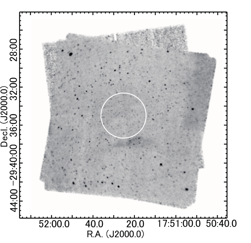
Figure 1.— Smoothed and exposure-corrected X-ray image (0.5–8.0 keV). All the ten data sets were stacked. The white circle at the center shows the region studied by Revnivtsev et al. (2009, 2011).

We retrieved pipeline products and reduced the data sets using the Chandra Interactive Analysis of Observations (CIAO) software package (Fruscione et al., 2006) version 4.2. We reprocessed the raw data to obtain an X-ray event list for each ObsID, in which we filtered events based on event grades, good time intervals, and energy bands (0.5–8.0 keV), and applied a background rejection algorithm to data taken with the very faint telemetry format. We then merged the ten event files into one. Figure 1 shows the combined ACIS-I images corrected for the non-uniformity of the exposure across the study field.

3. Analysis

3.1. Source Extraction

We first extracted point source candidates using the wavdetect algorithm in the CIAO package. We set the significance threshold at 2.5 $\times$ 10^-5, implying that one false positive detection would be expected at every 4 $\times$ 10⁴ trials. As a result, 2,596 source candidates were found. The number of our source candidates is nearly the same with that by Revnivtsev et al. (2009) in the same region.

For all the source candidates, we extracted source and background events using the ACIS Extract (AE; Broos et al. 2010) package version 2009-12-01. The source events were extracted from a region containing $\sim$90% of photons based on the simulated point spread function of each source, while the background events were extracted locally from an annulus around each source. When two source extraction regions overlap with each other, each region was shrunk so that the overlap disappeared. In the background regions, circles with a radius of 1.1 times the $\sim$99% encircled energy radius of each source candidate were masked. All these processes are automated in the AE package, which is useful to extract sources in the studied region with a high source surface number density possibly with underlying extended emission.

Table 2Chandra Catalog: Basic Source Properties

Source		Position				Extracted Counts					Characteristics
Seq	CXOU J	$\rm{R.\,A.}$	$\rm{Decl.}$	Err	$\theta$	$C_{\rm{net}}$	$\Delta C_{\rm{net}}$	$C^{\prime}_{\rm{bkg}}$	$C_{\rm{net,hard}}$	PSF	PS	$P_{\mathrm{B}}$	Anom	Var	EffExp	ME	Photo $F_{\rm{X}}$	$q_{1}$	$q_{2}$
#		(deg)	(deg)	(″)	(′)					Frac					(ks)	(keV)	(ergs cm-2 s-1)
(1)	(2)	(3)	(4)	(5)	(6)	(7)	(8)	(9)	(10)	(11)	(12)	(13)	(14)	(15)	(16)	(17)	(18)	(19)	(20)
1	175044.88$-$292837.6	267.687010	$-$29.477113	0.4	11.6	78.4	23.5	437.6	29.2	0.89	3.3	$-$3.9	….	b	486.5	1.5	1.6$\times$10-15	$-$0.80	0.63
2	175045.10$-$293431.4	267.687940	$-$29.575409	0.4	9.2	38.4	14.9	163.6	30.0	0.90	2.5	$-$2.7	g…	…	325.1	3.0	1.1$\times$10-15	$-$0.81	1.26
3	175045.10$-$293240.5	267.687950	$-$29.544603	0.3	9.7	56.1	19.1	279.9	17.7	0.89	2.9	$-$3.3	g…	…	535.5	1.5	2.4$\times$10-15	$-$0.31	1.63
4	175045.51$-$293222.4	267.689630	$-$29.539560	0.3	9.7	46.4	16.5	201.6	34.1	0.78	2.7	$-$3.1	g…	…	597.9	2.9	1.9$\times$10-15	$-$0.33	1.57
5	175045.86$-$293503.5	267.691120	$-$29.584322	0.3	9.1	60.6	16.5	190.4	52.7	0.90	3.6	$-$5.0	g…	…	417.5	2.7	3.0$\times$10-15	$-$0.39	1.67
6	175045.90$-$293208.7	267.691270	$-$29.535760	0.3	9.7	92.1	20.3	291.9	24.2	0.85	4.4	$<-$5	g…	…	639.9	1.4	1.5$\times$10-15	$-$0.88	0.96
7	175046.03$-$293539.1	267.691800	$-$29.594220	0.4	9.0	40.2	15.5	179.8	10.7	0.90	2.5	$-$2.7	g…	…	387.2	1.8	1.3$\times$10-15	$-$0.66	1.85
8	175046.07$-$293405.8	267.691960	$-$29.568297	0.3	9.2	69.0	19.2	270.0	46.8	0.90	3.5	$-$4.7	g…	…	570.4	2.4	2.0$\times$10-15	$-$0.46	1.40
9	175046.25$-$292947.1	267.692710	$-$29.496437	0.3	10.7	60.1	17.6	224.9	51.2	0.69	3.3	$-$4.3	….	b	678.2	3.3	2.5$\times$10-15	$-$0.22	1.35
10	175046.62$-$292935.0	267.694250	$-$29.493066	0.3	10.8	58.6	17.7	229.4	73.7	0.70	3.2	$-$4.1	….	b	677.5	5.2	3.9$\times$10-15	00.23	2.01
11	175047.08$-$293334.4	267.696170	$-$29.559558	0.3	9.1	48.4	19.9	316.6	8.2	0.90	2.4	$-$2.4	g…	…	679.6	1.2	6.3$\times$10-16	$-$0.96	1.12
12	175047.51$-$293733.0	267.697980	$-$29.625834	0.3	9.0	51.4	17.4	226.6	42.1	0.90	2.9	$-$3.3	g…	…	519.2	2.8	2.0$\times$10-15	$-$0.37	1.35
13	175048.28$-$293250.7	267.701180	$-$29.547440	0.2	9.0	148.7	22.4	321.3	125.7	0.90	6.5	$<-$5	….	a	714.8	3.5	4.8$\times$10-15	$-$0.18	1.34
14	175048.39$-$292816.1	267.701660	$-$29.471139	0.4	11.3	71.4	20.2	304.6	47.4	0.90	3.5	$-$4.5	g…	…	386.5	2.4	3.1$\times$10-15	$-$0.46	1.39
15	175048.54$-$293937.5	267.702280	$-$29.660423	0.3	9.5	102.3	19.1	235.7	82.1	0.90	5.2	$<-$5	g…	…	457.0	3.0	5.1$\times$10-15	$-$0.29	1.45
16	175048.65$-$293538.6	267.702740	$-$29.594083	0.2	8.5	127.2	18.6	194.8	79.1	0.80	6.6	$<-$5	g…	…	734.4	3.6	4.8$\times$10-15	$-$0.15	0.79
17	175048.86$-$293736.9	267.703620	$-$29.626938	0.3	8.8	73.8	20.0	296.2	30.3	0.90	3.6	$-$4.8	g…	…	698.8	1.9	1.4$\times$10-15	$-$0.65	0.84
18	175048.91$-$292906.9	267.703810	$-$29.485275	0.3	10.6	124.8	25.5	482.2	45.0	0.90	4.8	$<-$5	….	a	668.0	1.6	1.9$\times$10-15	$-$0.78	1.14
19	175048.95$-$293547.9	267.703980	$-$29.596661	0.2	8.5	82.7	16.4	165.3	51.4	0.76	4.9	$<-$5	….	a	752.1	2.5	2.1$\times$10-15	$-$0.43	0.77
20	175049.07$-$293803.6	267.704500	$-$29.634354	0.3	8.8	82.8	20.6	312.2	13.8	0.90	3.9	$<-$5	g…	…	702.2	1.6	1.3$\times$10-15	$-$0.79	1.45

Note. — Col.(1): X-ray catalog sequence number, sorted by R. A. Col.(2): IAU designation. Col.(3),(4): R. A. and Decl. in the equinox J2000.0. Col.(5): Estimated standard deviation of the position error. Col.(6): Off-axis angle. Col.(7),(8): Estimated net counts and errors extracted in 0.5–8.0 keV. Col.(9): Background counts in 0.5–8 keV. Col.(10): Estimated net counts extracted in the hard band (2.0–8.0 keV). Col.(11): Fraction of the PSF (at 1.497 keV) enclosed within the extraction region. A reduced PSF fraction (significantly below 90%) may indicate that the source is in a crowded region. Col.(12): Photometric significance. Col.(13): Logarithmic probability that the extracted counts (0.5–8.0 keV) are solely from background. Col.(14): Source anomalies: g = fractional time that source was on a detector (FRACEXPO from mkarf) is $<0.9$ Col.(15): Variability characterization based on K-S statistic (0.5–8.0 keV): a = no evidence for variability ($0.05<P_{KS}$); b = possibly variable ($0.005<P_{KS}<0.05$); c = definitely variable ($P_{KS}<0.005$). No value is reported for sources in chip gaps or on field edges. Col.(16): Effective exposure time: approximate time the source would have to be observed on-axis to obtain the reported number of counts. Col.(17): Background-corrected median photon energy (0.5–8.0 keV). Col.(18): Photometric flux estimate in the 0.5–8.0 keV band. Table 2 is published in its entirety in the electronic edition of the Astrophysical Journal. A portion is shown here for guidance regarding its form and content. Col.(19), (20): $q_{1}$ and $q_{2}$ quantile values indicating the spectral shape of each source (see text in § 4.1.1).

To select significant point sources from the candidates, we examined their validity based on their photometric significance (PS) and the probability of no source ($P_{\rm{B}}$). The PS is defined as the background-subtracted source counts ($C_{\mathrm{net}}$) divided by its background counts normalized by the area. $P_{\rm{B}}$ is the probability that the source is attributable to a background fluctuation assuming the Poisson statistics. We recognized the source to be valid if they satisfy both two criteria: $\mathrm{PS}$ $\geq$ 1.0 and $P_{\rm{B}}$ $\leq$ $1.0\times 10^{-2}$. As a result, we obtained 2,002 valid point sources. Table 2 tabulates the photometric properties of the first 20 sources, and the full source list is available in the on-line version. The X-ray sources can be referred following the International Astronomical Union (IAU) convention; e.g., CXOU J175044.88–292837.6 for the source sequence number 1 in Table 2.

3.2. Detection Completeness

We estimated the detection completeness averaged over the entire area in the following method. We generated events of 400 artificial sources using the marx event simulator at random positions across the image with a given flux. The events were merged with the observed events, from which point sources were detected using the same algorithm with the observed data. We derived the detection rate at each flux, which was changed from 10^-13 to 10${}^{-17}~{}{\rm ergs}\ {\rm cm}^{-2}\ {\rm s}^{-1}$ in the total (0.5–8.0 keV) and the hard (2–8 keV) bands. We assumed that the artificial sources have the same spectrum with the best-fit model describing the stacked spectrum of all point sources (§ 4.2). Figure 2 shows the detection rate as a function of flux. The rate is nearly complete (more than 97%) above $\sim$10${}^{-15.2}~{}{\rm ergs}\ {\rm cm}^{-2}\ {\rm s}^{-1}$ in the total band and $\sim$10${}^{-14.8}~{}{\rm ergs}\ {\rm cm}^{-2}\ {\rm s}^{-1}$ in the hard band.

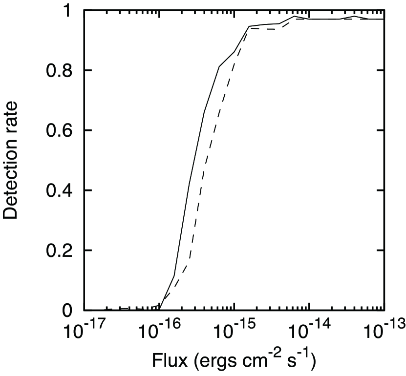
Figure 2.— Detection rate as a function of flux in 0.5–8.0 keV (solid) and in 2–8 keV (dashed).

3.3. Photometry

Because most of the detected sources are faint, we used the photometric information to characterize their spectral hardness (color) and flux based on a quantile method (Hong et al., 2004). We derived the median energy (ME) for each source, which is a proxy for the spectral hardness. The distribution of the ME of all sources is shown in Figure 3 (a).

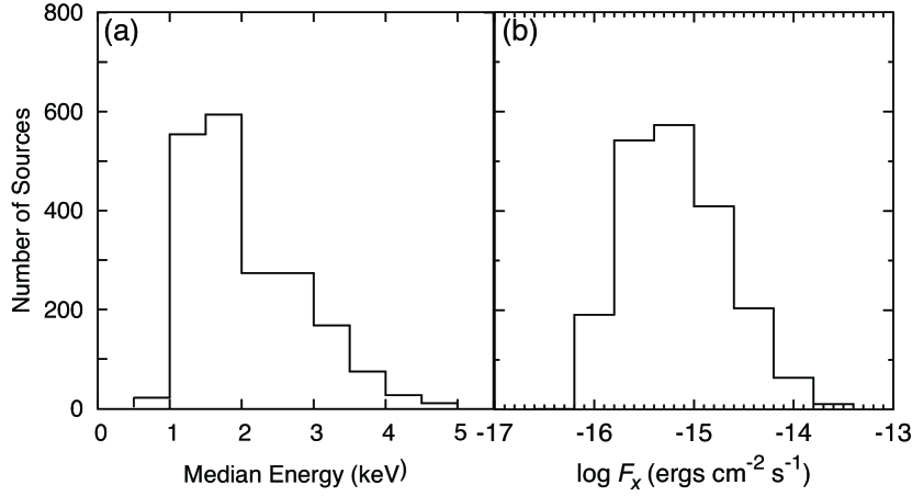
Figure 3.— Distribution of (a) median energy and (b) photometric flux in the 0.5–8.0 keV band for all sources.

We derived the flux of all sources using the photometric flux ($F_{\mathrm{ph}}$) defined as

$$F_{\mathrm{ph}}~{}({\rm ergs}\ {\rm cm}^{-2}\ {\rm s}^{-1})=1.6\times 10^{-9}~{}\frac{\mathrm{ME~{}(keV)}~{}C_{\mathrm{net}}~{}(\mathrm{s}^{-1})}{\mathrm{EA~{}(\mathrm{cm}^{2})}}~{},$$

in which EA is the energy-averaged effective area for each source. We derived both the total (0.5–8.0 keV) and the hard (2–8 keV) band photometric flux. Some sources have no hard-band photometric flux because of their lack of photons in the band. The distribution of $F_{\mathrm{ph}}$ is shown in Figure 3 (b). In order to check the consistency with the flux derived by spectral fitting (§ 3.5), we compared the flux estimates both by photometric and spectroscopic methods for 335 sources, for which spectral fitting result was available. The comparison shows that they are in a good agreement (Fig. 4). Hereafter, we use the photometric flux for all sources.

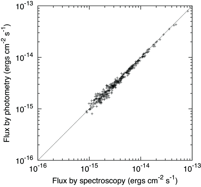
Figure 4.— Relation between two X-ray flux estimates for 335 sources, for which spectral fitting results are available. The vertical and horizontal axes represent the X-ray flux in the 0.5–8.0 keV estimated by the photometric and spectroscopic method, respectively. The dotted line represents the equal value between the two estimates.

3.4. Variability

In order to examine time variability in the count rate, we applied the Kolmogorov-Smirnov (KS) test for the sources with net counts more than 100 (355 sources in total), which we call bright sources. The test examines the degree of non-uniformity in the distribution of photon arrival times against a uniform distribution (or constant flux) using the $\chi^{2}$ statistics. Sources were removed if they were in the chip gaps or at the field edge in at least one observation, because the telescope dithering causes artificial variability.

The null hypothesis probability of the KS test was derived for each source in each of the ten observations. We defined the merged probability ($P_{\mathrm{KS}}$) for each source as the smallest value among the ten probabilities. Based on this, we divided sources into three sets: (a) $P_{\mathrm{KS}}\geq 5\times 10^{-2}$ for non-variable sources (109 sources), (b) $5\times 10^{-3}\leq P_{\mathrm{KS}}<5\times 10^{-2}$ for marginally variable sources (68 sources), and (c) $P_{\mathrm{KS}}<5\times 10^{-3}$ for variable sources (34 sources).

By looking at the light curve of variable sources, we noticed that some sources show a typical flare-like flux variation of fast rise and slow decay. The KS test does not consider the profile of the variation in the light curve, so we picked up flare-like sources by setting a different criterion that the contrast of the maximum to minimum count rate is larger than 10 in at least one observation. In this manner, we selected nine flare-like sources, which are shown in Figure 5.

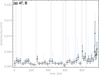
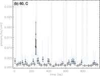
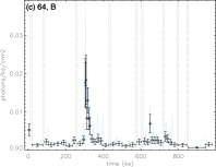
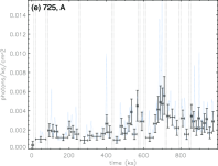
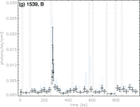
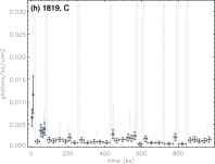
Figure 5.— Concatenated light curves for sources with flare-like variability. The light curves show variations in count rate (black histograms are binned and blue curves are adaptively smoothed). Time intervals between observations are indicated by black dotted vertical lines. The top left labels show the sequence number in Table 2 and the group (§ 4.1) of each source.

3.5. Spectroscopy

For the bright sources, we constructed the background-subtracted spectra and generated instrumental response files; i.e., redistribution matrix function (RMF) of the detector and auxiliary response file (ARF) of the telescope. We derived the best-fit parameters of the spectral models using the $\chi^{2}$ statistics.

For the spectral models, we used an interstellar absorption model (tbabs; Wilms et al. 2000) convolved with either of the two continuum models: an optically-thin thermal plasma model (apec; Smith et al. 2001) and a power-law model to represent the thermal and non-thermal spectra, respectively. Free parameters for the thermal model are the absorption column ($N_{\rm H}$), the plasma temperature ($k_{\rm{B}}T$), and the flux ($F_{\rm{X}}$) in the 0.5–8.0 keV band, while those for the power-law model are the absorption column ($N_{\rm H}$), the photon index ($\Gamma$), and the flux ($F_{\rm{X}}$) in the 0.5–8.0 keV band. For the plasma model, we fixed the abundance to the value in Güdel et al. (2007). We regarded the fitting to be unsuccessful if the reduced $\chi^{2}$ was larger than 1.5 or the best-fit values were unphysical; i.e., $\Gamma>3$ in the power-law fitting and $k_{\rm{B}}T>15$ keV in the apec fitting. For sources with unsuccessful fitting in both models, we also tried a plasma model with two different temperatures. For sources with successful fitting in both models, we adopted the result with the smaller reduced $\chi^{2}$ value.

As a result, 71 sources were successfully fitted with the one-temperature plasma model, 50 sources with the two-temperature plasma model, and 158 sources with the power-law model. Figure 6 shows the spectra and the best-fit models for all sources with more than 1000 net counts. Tables 3 and 4 show the best-fit parameters for the one-temperature and power-law fitting of these sources, respectively.

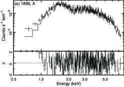
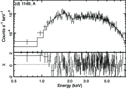
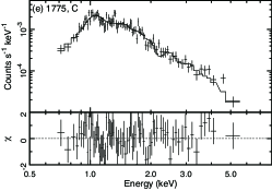
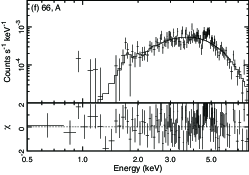
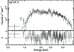
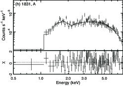
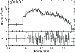
Figure 6.— X-ray spectra of the sources with more than 1000 net counts in the order of the total counts. The top left labels show the sequence number in Table 2 and the group (§ 4.1) of each source. Thermal or non-thermal models are employed to fit the spectra. Grouped data are shown in the upper panels, which are over-plotted with the best-fit model convolved with the instrumental response. The lower panels show the residuals of the data to the fit. The best-fit parameters can be found in Tables 3 and 4.

Table 3Thermal fittings for the X-ray sources with source counts over 1000

Source				Spectral Fit			X-ray Flux
Seq.	CXOU J	$C_{\mathrm{t,net}}$	Signif.	$\log N_{\mathrm{H}}$	$kT_{1}$	$kT_{2}$	$F_{\mathrm{s}}$	$F_{\mathrm{h}}$	$F_{\mathrm{h,c}}$	$F_{\mathrm{t}}$	$F_{\mathrm{t,c}}$	$\chi^{2}$/d.o.f.
#				(cm-2)	(keV)	(keV)	(ergs cm-2 s-1)
(1)	(2)	(3)	(4)	(5)	(6)	(7)	(8)	(9)	(10)	(11)	(12)	(13)
287	175107.66$-$294037.3	3252.3	55.1	$21.6_{-0.07}^{+0.07}$	$0.3_{-0.1}^{+0.1}$	$3.9_{-0.5}^{+0.7}$	3.6e-14	2.6e-14	2.6e-14	5.0e-14	5.2e-14	129.30/131
1775	175148.91$-$293505.6	1779.1	40.7	$21.6_{-0.07}^{+0.07}$	$1.5_{-0.1}^{+0.1}$	…	1.1e-14	8.1e-15	8.6e-15	1.9e-14	3.0e-14	103.52/078

Note. — 1: For convenience, cols. (1)–(4) reproduce the source identification, net counts, and photometric significance data from Table 1, which are sorted by the number of counts. 2: All fits used the source model “tbabs*vapec” in XSPEC abundances frozen at the values relative to Anders & Grevesse (1989), scaled to Wilms et al. (2000), using the tbabs absorption code in XSPEC. Cols. (5), (6), and (7) present the best-fit values for the extinction column density and plasma temperature parameters. Uncertainties represent 90% confidence intervals. More significant digits are used for uncertainties $<$0.1 in order to avoid large rounding errors; for consistency, the same number of significant digits is used for both lower and upper uncertainties. Uncertainties are missing when XSPEC was unable to compute them or when their values were so large that the parameter is effectively unconstrained. Fits lacking uncertainties, fits with large uncertainties, and fits with frozen parameters should be viewed merely as splines to the data to obtain rough estimates of luminosities; the listed parameter values are not robust. 3: X-ray flux derived from the model spectrum are presented in cols. (8)–(12): (s) soft band (0.5–2 keV); (h) hard band (2–8 keV); (t) total band (0.5–8 keV). Absorption-corrected fluxes are subscripted with a $c$. Cols. (8) and (12) are omitted when $\log N_{\mathrm{H}}>22.5$ cm^-2 since the soft band emission is essentially unmeasurable.

Table 4Power-law fitting for the X-ray sources with source counts over 1000

Source				Spectral Fit			X-ray Flux
Seq.	CXOU J	$C_{\mathrm{t,net}}$	Signif.	$\log N_{\mathrm{H}}$	$\Gamma$	$\log N_{\Gamma}$	$F_{\mathrm{s}}$	$F_{\mathrm{h}}$	$F_{\mathrm{h,c}}$	$F_{\mathrm{t}}$	$F_{\mathrm{t,c}}$	$\chi^{2}$/d.o.f.
#				(cm-2)			(ergs cm-2 s-1)
(1)	(2)	(3)	(4)	(5)	(6)	(7)	(8)	(9)	(10)	(11)	(12)	(13)
1895	175154.71-292806.1	6440.6	77.1	$22.0_{-0.01}^{+0.01}$	1.8${}_{-0.1}^{+0.1}$	$-4.26_{-0.06}^{+0.06}$	1.7e-14	1.4e-13	1.7e-13	1.6e-13	2.9e-13	300.71/244
438	175113.70-293110.1	4325.4	64.4	$22.5_{-0.04}^{+0.04}$	1.5${}_{-0.1}^{+0.1}$	$-4.53_{-0.08}^{+0.08}$	5.8e-15	1.1e-13	1.3e-13	1.2e-13	2.0e-13	196.80/203
1149	175131.68-292957.0	2908.3	52.5	$22.4_{-0.06}^{+0.06}$	1.3${}_{-0.1}^{+0.1}$	$-4.87_{-0.09}^{+0.10}$	4.7e-15	7.8e-14	8.7e-14	8.2e-14	1.2e-13	137.31/142
66	175054.26-294327.4	1600.2	46.2	$22.7_{-0.05}^{+0.04}$	1.5${}_{-0.2}^{+0.2}$	$-4.87_{-0.09}^{+0.10}$	7.0e-16	8.0e-14	9.4e-14	8.0e-14	9.6e-14	128.96/110
33	175051.16-293419.5	1469.3	34.5	$22.4_{-0.09}^{+0.09}$	1.7${}_{-0.2}^{+0.3}$	$-4.92_{-0.2}^{+0.2}$	3.7e-15	3.7e-14	4.0e-14	4.1e-14	5.7e-14	88.60/071
1831	175151.29-293310.3	1447.3	36.3	$22.3_{-0.10}^{+0.09}$	$0.65_{-0.2}^{+0.2}$	$-5.51_{-0.1}^{+0.1}$	1.8e-15	4.8e-14	5.2e-14	5.0e-14	5.8e-14	113.47/078
1252	175134.06-293103.9	1390.3	36.0	$22.1_{-0.08}^{+0.08}$	1.6${}_{-0.2}^{+0.2}$	$-5.18_{-0.09}^{+0.10}$	3.9e-15	2.5e-14	2.6e-14	2.9e-14	4.1e-14	75.74/074
1869	175153.33-294245.0	1202.7	30.0	$22.4_{-0.1}^{+0.1}$	1.0${}_{-0.3}^{+0.3}$	$-5.30_{-0.2}^{+0.2}$	3.3e-15	5.0e-14	5.1e-14	5.3e-14	5.8e-14	60.59/058

Note. — 1: For convenience, cols. (1)–(4) reproduce the source identification, net counts, and photometric significance data from Table 1, which are sorted by the number of counts. 2: All fits used the source model “tbabs*powerlaw” in XSPEC. Cols. (5) and (6) present the best-fit values for the extinction column density and power law photon index parameters. Col. (7) presents the power law normalization for the model spectrum. Uncertainties represent 90% confidence intervals. More significant digits are used for uncertainties $<$0.1 in order to avoid large rounding errors; for consistency, the same number of significant digits is used for both lower and upper uncertainties. Uncertainties are missing when XSPEC was unable to compute them or when their values were so large that the parameter is effectively unconstrained. Fits lacking uncertainties, fits with large uncertainties, and fits with frozen parameters should be viewed merely as splines to the data to obtain rough estimates of luminosities; the listed parameter values are unreliable. 3: X-ray Flux derived from the model spectrum, assuming a distance of 8.5 kpc, are presented in cols. (8)–(12): (s) = soft band (0.5–2 keV); (h) hard band (2–8 keV); (t) total band (0.5–8 keV). Absorption-corrected fluxes are subscripted with a $c$. Cols. (8) and (12) are omitted when $\log N_{\mathrm{H}}>22.5$ cm^-2 since the soft band emission is essentially unmeasurable.

4. Discussion

We first attempt to group all the detected X-ray sources in § 4.1 based on the X-ray color-color diagram. After establishing these groups, we examine the X-ray properties of each group (§ 4.2). We then discuss likely classes for sources in each group (§ 4.3) and evaluate their contribution to the GRXE (§ 4.4).

4.1. Grouping

We constructed an X-ray color-color diagram (Hong et al., 2004) using the quantiles ($E_{25}$, $E_{{50}}$, and $E_{75}$) characterizing the spectral shape of each source. Here, $E_{x}$ (keV) is the energy below which $x$% of photons reside in the energy-sorted event list. $E_{50}$ is equivalent to the median energy. We first normalized these parameters as

$$Q_{x}=\frac{E_{\rm{x}}-E_{\rm{min}}}{E_{\rm{max}}-E_{\rm{min}}},$$ (1)

in which $E_{\rm{min}}$ and $E_{\rm{max}}$ are 0.5 and 8 keV, respectively. We then took ratios of two parameters as $q_{1}=\log_{10}Q_{\rm{50}}/\left(1-Q_{\rm{50}}\right)$ and $q_{2}=3Q_{\rm{25}}/Q_{\rm{75}}$ for all the sources. Here, the $q_{1}$ value indicates the degree of photon spectrum being biased toward the higher ($q_{1}>0$) or lower ($q_{1}<0$) energy end (hard or soft spectra), and the $q_{2}$ value indicates the degree of photon spectrum being less ($q_{2}>1$) or more ($q_{2}<1$) concentrated around the peak (broad or narrow spectra).

Figure 7 shows the color-color diagram using $q_{1}$ and $q_{2}$ of all the sources. In order to put the diagram into context, we simulated the quantiles of optically-thin thermal emission attenuated by interstellar photoelectric absorption. We used the bremss model for the emission and the tbabs model for the absorption with varying temperatures and column densities.

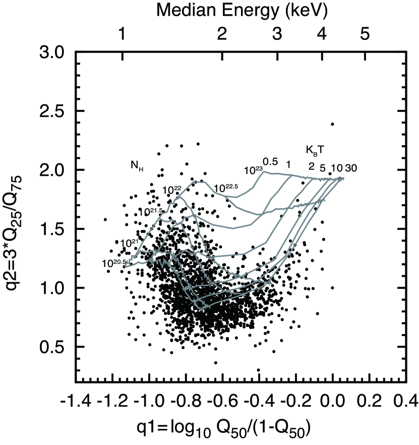
Figure 7.— X-ray color-color diagram of all detected X-ray sources. The converted median energy is shown in the upper $x$-axis. We also display a grid of thermal plasma spectra attenuated by interstellar absorption with various parameter combinations. The labels indicate the values of the plasma temperature ($k_{\rm{B}}T$) for 0.5, 1, 2, 5, 10, and 30 keV and the extinction column ($N_{\rm H}$) for 10^20.5, 10²¹, 10^21.5,  10²², and 10^22.5 cm^-2. In the simulation, background events were not included, so the grid should be considered only as a reference showing the relative parameter changes.

In the plot, sources are distributed from side to side with a main concentration around ($q_{1}$, $q_{2}$) $=$ ($-$0.8, 1.0). It appears that the scatter is extended in the upward and rightward directions from the main concentration. We examine if these branches have any physical basis by looking at count-stratified color-color diagrams (§ 4.1.1) and the results of bright sources (§ 4.1.2 and § 4.1.3) before dividing all sources into groups by a statistical approach (§ 4.1.4).

4.1.1 Count-Stratified Diagram

The color-color diagram does not represent the flux of sources. Therefore, we constructed the diagram for different count ranges (Fig.  8). The scatter plots exhibit quite a different morphology among the four count ranges. In the lowest count range (Fig.  8a), the sources are scattered in the main concentration and the upward branch. As the count increases, the sources in the upward branch disappear and are gradually replaced with sources in the rightward branch (Fig.  8b) to form a V-shaped distribution (Fig.  8c). In the highest count range (Fig.  8d), the sources are only seen in the rightward branch.

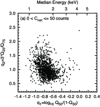
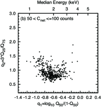
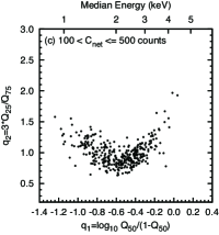
Figure 8.— X-ray color-color diagram for different count ranges. The symbols are the same with Figure 7.

4.1.2 Variability of bright Sources

In the variability analysis of the bright sources (§ 3.4), some show flare-like variability. Figure 9 shows where they are located in the color-color diagram. We omitted the sources with less than 100 counts, as they are too weak to examine their variability; the faintest source with a statistically significant variability has a net count of 100.5 (§ 3.4). It is interesting to find that all but one flare-like variable sources are found along the left arm of the V-shaped distribution, although the variable sources are equally found in both arms.

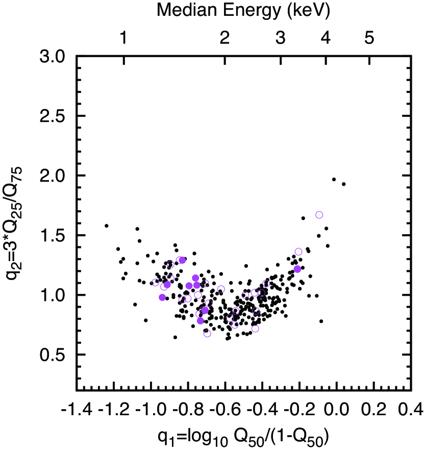
Figure 9.— X-ray color-color diagram of the bright sources (Cnet $>$ 100 counts). Variable sources are shown with magenta circles, among which flare-like variable sources are filled.

4.1.3 Spectra of bright Sources

In the spectral analysis of the bright sources (§ 3.5), some sources are described by thermal spectra and others by non-thermal spectra. For sources with more than 1,000 counts (Fig.  6), two sources are thermal and eight are non-thermal. Figure 10 shows where they are located in the color-color diagram. The bimodality is clearly seen, in which thermal and non-thermal sources are exclusively found respectively in the left and right arm of the V-shaped distribution.

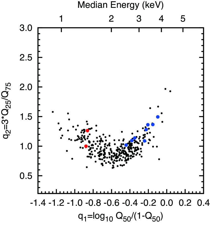
Figure 10.— X-ray color-color diagram of the bright sources (Cnet $>$ 100 counts). Sources with a thermal spectrum (Fig. 6) are shown with red circles, while those with a non-thermal spectrum are shown with blue circles.

4.1.4 Statistical Treatment

From the discussion above, it is reasonable to assume that the sources consist of three representative groups that can be separated by the position in the diagram: main concentration, upward branch, and rightward branch. In order to define the boundaries in an objective manner, we employed the $k$-means clustering algorithm using the mlpy script. Given the number of groups, the algorithm determines a centroid of each group and the sources that belong to the group iteratively, so that the sum of the distances from each source to the centroid becomes minimum.

Using this method, we divided the 2,002 sources into three groups (group A, B, and C) by their position in the diagram (Figure 11). The resultant division was mostly consistent with its appearance; the group A for the rightward branch, B for the main concentration, and C for the upward branch. Some exceptions are seen; e.g., two sources at the tip of the rightward branch were divided into the group C, rather than A, which is conceivable in such an algorithm. The two sources are quite faint comprising only $<$0.5% of the total net count of the groups A and C, so they do not affect the composite spectrum of the groups discussed below.

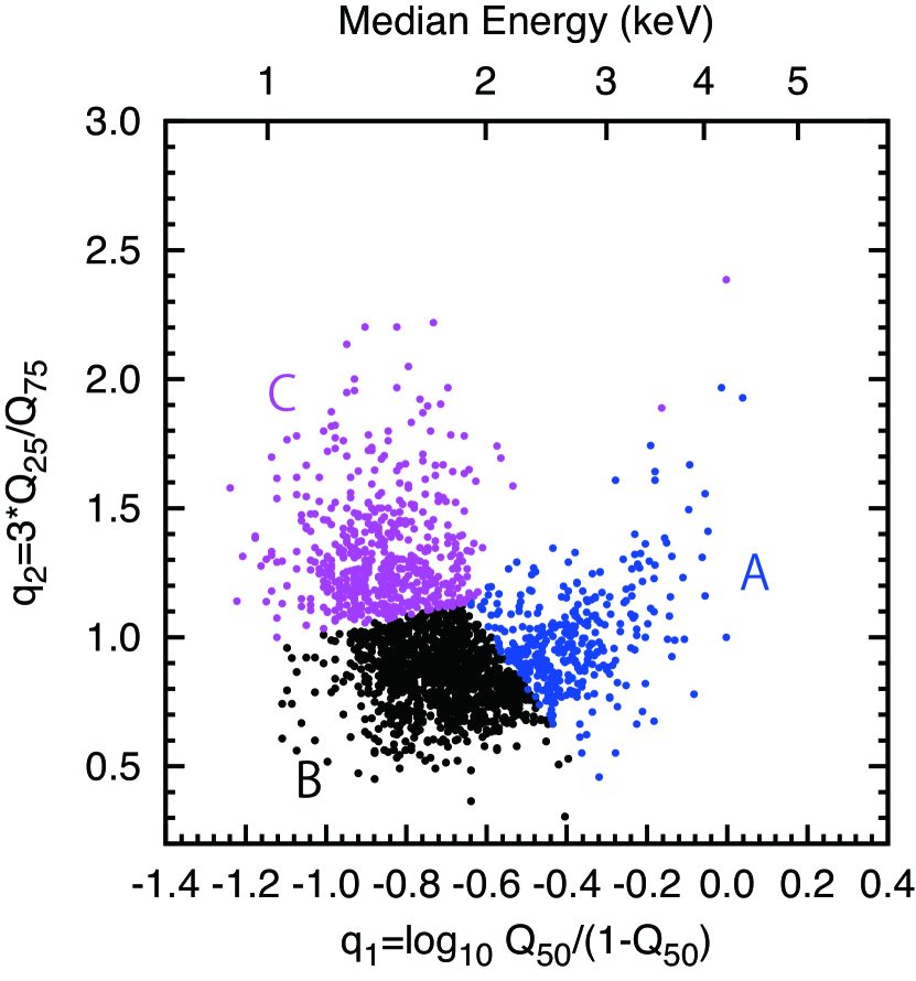
Figure 11.— X-ray color-color diagrams of all sources color-coded depending on their statistically-defined classes. The other symbols follow Figure 7.

4.2. X-ray Properties of Each Group

4.2.1 Fe K Feature

We made composite spectra of the three groups A, B. and C using the CIAO tool combine_spectra. The tool makes background-subtracted spectra as well as count-weighted ARFs and RMFs of multiple sources.

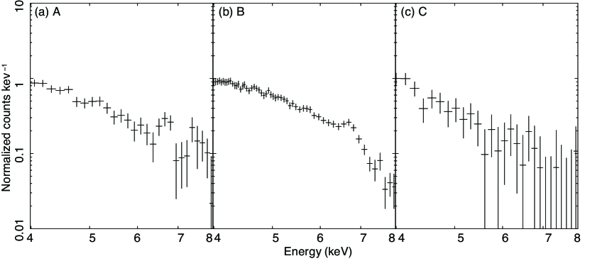
Figure 12.— Fe K feature in the combined spectra of point sources in the group (a) A, (b) B, and (c) C. The spectra are normalized at 4 keV.

Figure 12 shows the enlarged view in the 4–8 keV band, in which the Fe K feature appears differently for each group. We characterized the feature by fitting the 4–8 keV spectrum using a power-law plus a Gaussian model. The free parameters were the power-law index and normalization, and the Gaussian line center, width, and normalization. For the group C, the Gaussian component was not required, so we only constrained the upper limit to the emission. The result is shown in Table 5. For the best-fit value of the Gaussian line center, we found no significant differences among different groups.

Table 5Best-fit parameters of the power-law $+$ Gaussian model for the Fe K feature

Group	$E_{\mathrm{gau}}$	EWgau	$F_{\mathrm{pow}}$/$10^{-13}$	$f_{\mathrm{pow}}^{\mathrm{(PS)}}$	$f_{\mathrm{pow}}^{\mathrm{(Total)}}$	$F_{\mathrm{gau}}$/$10^{-13}$	$f_{\mathrm{gau}}^{\mathrm{(PS)}}$	$f_{\mathrm{gau}}^{\mathrm{(Total)}}$
	(keV)	(eV)	(${\rm ergs}\ {\rm cm}^{-2}\ {\rm s}^{-1}$)			(${\rm ergs}\ {\rm cm}^{-2}\ {\rm s}^{-1}$)
A	6.69${}_{-0.05}^{+0.06}$	268${}_{-99}^{+244}$	012.02${}_{-0.54}^{+0.58}$	0.68${}_{-0.03}^{+0.04}$	0.44${}_{-0.02}^{+0.02}$	0.98${}_{-0.12}^{+0.12}$	0.62${}_{-0.08}^{+0.08}$	0.26${}_{-0.03}^{+0.03}$
B	6.70${}_{-0.08}^{+0.08}$	413${}_{-216}^{+263}$	05.01${}_{-0.55}^{+0.61}$	0.28${}_{-0.03}^{+0.04}$	0.18${}_{-0.02}^{+0.02}$	0.50${}_{-0.19}^{+0.34}$	0.32${}_{-0.12}^{+0.22}$	0.13${}_{-0.05}^{+0.09}$
C	$\cdots$	$\cdots$	00.68${}_{-0.12}^{+0.19}$	0.04${}_{-0.01}^{+0.01}$	0.02${}_{-0.01}^{+0.01}$	$<$0.04	$\cdots$	$\cdots$
All PS	6.69${}_{-0.04}^{+0.05}$	321${}_{-122}^{+116}$	17.18${}_{-0.70}^{+0.71}$	$\cdots$	$\cdots$	1.58${}_{-0.51}^{+0.60}$	$\cdots$	$\cdots$
Total emission	6.74${}_{-0.04}^{+0.05}$	581${}_{-131}^{+100}$	27.22${}_{-0.54}^{+0.54}$	$\cdots$	$\cdots$	3.82${}_{-0.51}^{+0.50}$	$\cdots$	$\cdots$

The characterization of the Fe K feature was conducted also for the composite spectrum of all point sources and the total emission extracted from the entire field. The fractional contribution of the continuum (4–8 keV) and the Fe K band emission was derived separately for each group. The fraction of point sources among the entire emission is smaller than that reported ($\sim$80%) in Revnivtsev et al. (2009), which is presumably due to our lower sensitivity on average by using the entire field rather than the central part of the observations.

The presence of the Fe K feature in the combined spectrum of the group A sources (Fig. 12a) seemingly contradicts the result of the spectral fitting of individual bright sources (§ 3.5), because most of the bright sources in the group A hardly show signatures of the Fe K feature. Among the brightest ten sources shown in Figure 6, eight are group A sources (source numbers 1895, 438, 1149, 66, 33, 1831, 1252, and 1869), all of which are fitted with a power-law model (Table 4). This strongly suggests that the presence of the Fe K feature depends on the source flux within the group A. No such apparent contradiction was found in the other groups.

In order to investigate the flux dependence for the Fe K contribution, we constructed spectra stacking flux-sorted sources cumulatively from the brightest source toward the fainter end by increasing the source number by 1 (1–20), by 10 (20–40), and by 20 (40–) at each step. In other words, the composite spectrum was made for the brightest 1, 2, …, 20, 30, 40, 60, 80, … sources. We then applied a power-law plus a Gaussian model for the spectrum generated at each step to derive the EW of the Fe K feature. Figure 12 (a) shows the EW value against the decreasing flux. At the brightest end ($>$2$\times$10^-14 ${\rm ergs}\ {\rm cm}^{-2}\ {\rm s}^{-1}$), the EW is consistent with being zero, which gradually increases as the threshold flux decreases and eventually levels off. This suggests that different classes of sources are dominant in the brighter and fainter end of the flux and their ratio gradually changes along the flux.

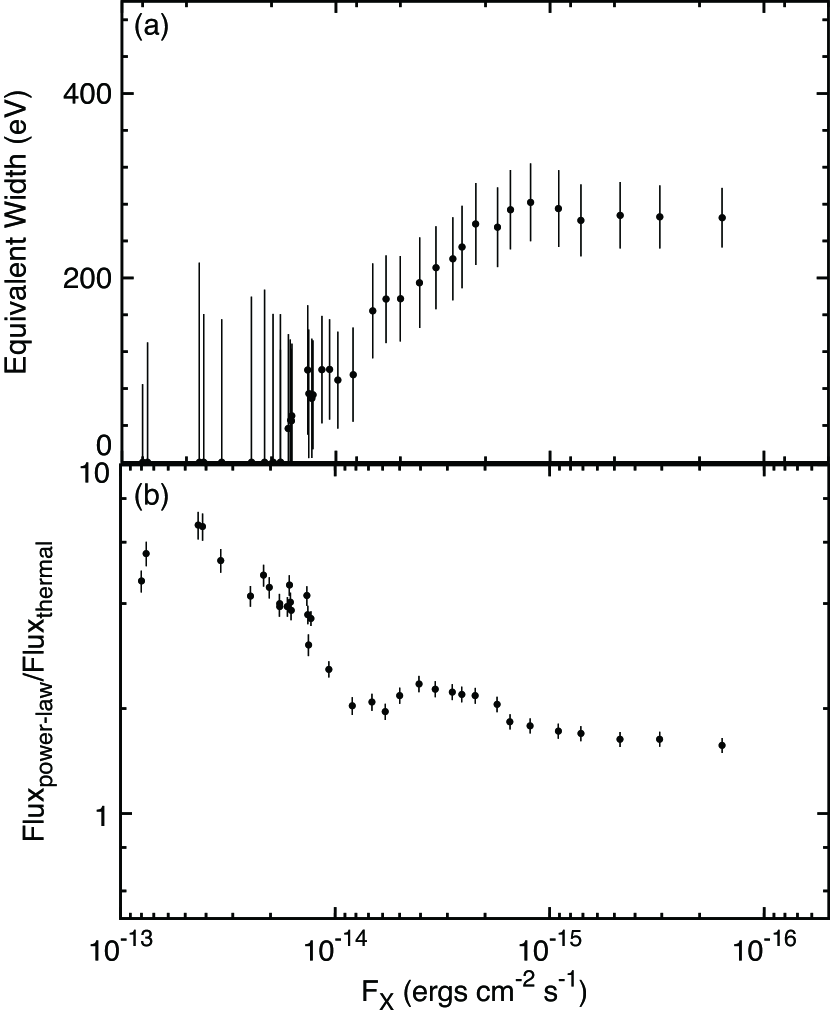
Figure 13.— (a) EW of the Fe K feature and (b) the 2–8 keV flux ratio of the power-law ($F_{\mathrm{power-law}}$) versus thermal ($F_{\mathrm{thermal}}$) components against the decreasing flux in 2–8 keV above which the cumulative combined spectra were constructed. The 1$\sigma$ statistical uncertainty is shown for each data point.

4.2.2 Global Spectral Fitting

We performed global spectral fitting using the entire energy band (0.5–8.0 keV) for the composite spectrum for each group (Fig. 11) in a similar manner for the individual bright sources (§ 3.4). For the thin-thermal plasma model, we fixed the abundance to that adopted in Güdel et al. (1999).

Group A

For the group A spectrum, neither a power-law nor a thin-thermal plasma model did not reproduce the spectrum well respectively because of the excess emission at 6.7 keV or a flatness of the continuum. In fact, these two are a signature respectively of a thin-thermal and a power-law model, so we fitted the spectrum with a combination of the two, which was successful. The best-fit model are given in Figure 14, whereas the best-fit parameters are in Table 6.

The EW of the Fe K feature becomes larger as the flux decreases (§ 4.2.1), which suggests that the thermal component becomes stronger against the non-thermal component as the flux decreases. In order to investigate this trend, we fitted the cumulatively stacked spectra (§ 4.2.1) with a power-law plus an optically-thin thermal plasma model. The free parameters are the normalization of the two components, and the other parameters were fixed to the values obtained in the fitting of all group A source (Table 6). As is expected, the flux ratio of the two components $F_{\mathrm{power-law}}$/$F_{\mathrm{thermal}}$ starts to decrease at $\sim$10^-14 ${\rm ergs}\ {\rm cm}^{-2}\ {\rm s}^{-1}$ (Fig. 13b), which is consistent with the EW trend (Fig. 13a).

Group B & C

For the group B spectrum, several emission lines are seen, including the 6.7 keV emission from Fe XXV and 2.5 keV from S XV. This set of emission lines indicates a multiple-temperature plasma, and indeed the spectrum was reproduced well with two thin-thermal plasma components, but not with one component. The free parameters are the plasma temperature, metallicity, and absorption column. The metallicity was the same among all the metals and was constrained to be the same between the two plasma components.

For the group C spectrum, several emission lines are also seen. Unlike the group B sources, the Fe XXV emission at 6.7 keV is absent. We fitted the spectrum using the same model with group B and obtained the best-fit parameters in Table 6.

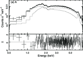
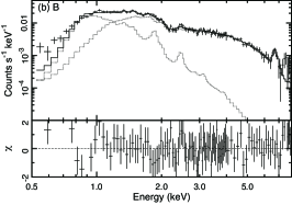
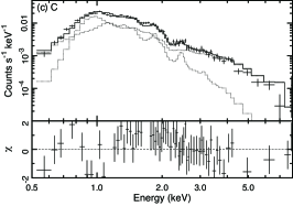
Figure 14.— Composite spectra and the best-fit global model of the group (a) A, (b) B, and (c) C. The symbols follow Figure 6.

Table 6Best-fit parameters for global spectral model in 0.5–8.0 keV

Group	$N_{\rm H}$(1)	$k_{\rm{B}}T$(1)	$N_{\rm H}$(2)	$k_{\rm{B}}T$(2)	Z	$\Gamma$	$N_{\mathrm{apec}}^{(1)}$/$N_{\mathrm{apec}}^{(2)}$	$\chi^{2}$/d.o.f.
	(1022 cm-2)	(keV)	(1022 cm-2)	(keV)
A	1.09${}_{-0.50}^{+0.39}$	6.65${}_{-3.03}^{+3.24}$	2.46${}_{-0.58}^{+2.35}$	$\cdots$	0.97${}_{-0.32}^{+0.36}$	1.29${}_{-0.40}^{+0.18}$	$\cdots$	0205.36/504
B	0.75${}_{-0.05}^{+0.06}$	0.74${}_{-0.45}^{+0.54}$	0.80${}_{-0.18}^{+0.22}$	7.87${}_{-4.84}^{+1.86}$	0.99${}_{-0.29}^{+0.33}$	$\cdots$	0.47${}_{-0.14}^{+0.18}$	098.68/103
C	0.70${}_{-0.11}^{+0.18}$	0.78${}_{-0.03}^{+0.04}$	0.04${}_{-0.04}^{+0.05}$	4.50${}_{-0.35}^{+0.65}$	0.15${}_{-0.12}^{+0.16}$	$\cdots$	6.70${}_{-0.20}^{+0.13}$	085.86/102

4.2.3 The $\log N$–$\log S$ Curve

We made the $\log N$–$\log S$ curve separately for all point sources and those for each group (solid histograms in Fig. 15). The curves were constructed in the hard band. For the group A curve, we divided the cumulative number into two, representing the power-law and plasma sources by using the smoothed flux ratio curve as a function of flux (Fig. 13b). We did not correct the $\log N$–$\log S$ curve because we do not discuss the absolute value of the vertical axis of the $\log N$–$\log S$ curve.

It is expected that a certain fraction of point sources are extra-galactic sources, which we represent with the $\log N$–$\log S$ curve constructed in a Chandra deep field (CDF; Rosati et al. 2002). Since the extra-galactic sources in our study field are more absorbed than those in the CDF at a high Galactic latitude, we took into account the flux reduction due to the Galactic absorption with a column density of 10²² cm^-2 assuming a typical spectral shape of sources in the CDF (Tozzi et al., 2006). The additional Galactic column density is a typical best-fit value among the sources with spectral fitting (Table 3).

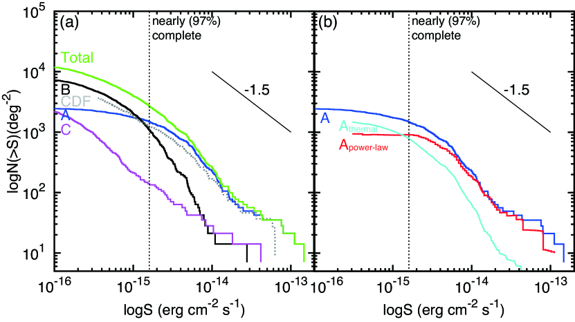
Figure 15.— Cumulative source surface number density $N$ (deg^-2) against the flux $S$ ${\rm ergs}\ {\rm cm}^{-2}\ {\rm s}^{-1}$ in the hard band (2–8 keV) separately for (a) all point sources (green) and those belonging to the group A (blue), B (black), and C (magenta), and (b) those decomposed into power-law (A_power-law; red) and thermal (A_thermal; cyan) sources. The curve for extra-galactic sources with an absorption of $\sim$10²² cm^-2 is shown with the gray dotted curve using the CDF data (Rosati et al., 2002) in (a). The slope of –1.5 for spatially uniform distribution is shown at the top right. All curves are not corrected for the detection completeness. The nearly (97%) completeness limit is shown with the vertical dashed line.

4.3. Likely Populations

We now discuss likely classes of the X-ray point sources in each group based on the results presented above. The transition from one class to another is continuous along the color and flux, so the groups are naturally a mixture of sources of different classes. We thus discuss the likely classes of sources that constitute the majority of each group.

First, we consider that the group A sources are mostly a mixture of AGNs and WD binaries, each responsible for the power-law and thermal plasma component in the composite spectrum (Fig. 14a). For the power-law component of the group A, the $\log N$–$\log S$ curve (Fig. 15) matches quite well to the completeness limit (Fig. 2) with that obtained in the CDF (Rosati et al., 2002). In the spectral fitting, the power-law component has a spectral index of 1.29${}^{+0.18}_{-0.40}$ (Table 6), which is similar to the typical spectral form of AGNs with a power-law index of about 1.63$\pm$0.13 in the X-ray band regardless of their types and luminosities (e.g., Rosati et al. 2002; Charles & Seward 1997).

For the thermal component of the composite spectrum (Fig. 14a) of the group A, a strong Fe K feature and a 7 keV temperature plasma (Table 6) are seen. Both of these features are observational characteristics of magnetic CVs (Ezuka & Ishida, 1999). Other classes of white dwarf (WD) binaries, such as dwarf novae, pre-CVs, and symbiotic stars, may also be considered for the likely classes. Pre-CVs are poorly recognized class of sources, which are detached binaries of a WD and a late-type star, unlike conventional CVs that are semi-detached systems. Some of them show strong Fe K emission in the hard X-rays (Matranga et al., 2012). Likewise, some symbiotic stars are also known to show strong Fe K emission feature (Eze et al., 2012). In fact, Morihana (2012) showed near-infrared spectra of selected X-ray sources presented in this paper, in which some thermal A sources do not exhibit the Br$\gamma$ emission that is typical for the conventional CVs (Dhillon et al., 1997). We thus consider that pre-CVs and symbiotic stars, most of which do not show the Br$\gamma$ emission (Howell et al., 2010; Schmidt & Mikołajewska, 2003), also account for at least some fraction of the thermal source population in the group A.

The group B and C sources are Galactic sources with a soft thermal spectrum, and we consider that most of them are likely to be X-ray active stars. The composite spectra of the two groups were fitted with two plasma components (Fig. 14 and Table 6). The lower temperature component and its absorption column are quite similar between the two, indicating that the difference between the B and C are not their typical distances. On the contrary, the higher temperature component is significantly higher for the group B; it is is high enough to produce a strong Fe K feature at 6.7 keV, which is absent in the C spectrum. We speculate that the difference between B and C is that most C sources represent active binary stars in the quiescence, while most B sources represent those during flares. Although most flare-like variable sources are indeed group B sources (Fig.  9), this can be a statistical bias because the group C sources are systematically fainter than group B sources (Fig.  8).

4.4. Comparison with Previous Studies and Contribution to GRXE

We have constructed a $\log N$–$\log S$ curve in the 2–8 keV band down to the flux $\sim$10^-16 ${\rm ergs}\ {\rm cm}^{-2}\ {\rm s}^{-1}$ using the CBF data (§ 4.2). Several major groups of sources account for different fractions of the GXRE continuum and Fe K$\alpha$ emission in different flux ranges.

For the continuum emission, low-mass X-ray binaries dominate in the flux range above $\approx$10^-12 ${\rm ergs}\ {\rm cm}^{-2}\ {\rm s}^{-1}$ in the $\log N$–$\log S$ curve, as was found in previous studies (e.g., Hands et al. 2004). These bright Galactic sources saturates, and background AGNs emerge as the most dominant class of sources in the next flux range of $\approx$10^-12–10^-14 ${\rm ergs}\ {\rm cm}^{-2}\ {\rm s}^{-1}$. The dominance of AGNs over Galactic population in this flux range was also discussed by Ebisawa et al. (2001, 2005); Hands et al. (2004); Revnivtsev et al. (2009); Motch et al. (2010). Below $\approx$10^-14 ${\rm ergs}\ {\rm cm}^{-2}\ {\rm s}^{-1}$, Galactic sources start to dominate the $\log N$–$\log S$ curve again. We decomposed the $\log N$–$\log S$ curve of the group A sources into non-thermal (AGNs in our speculation) and plasma sources (WD binaries) by utilizing the increasing EW of the Fe K$\alpha$ emission in the composite spectra along the decreasing flux. The group A thermal sources (WD binaries) and the group B sources (X-ray active stars) are the major contributers in this flux range. These two Galactic classes are also proposed to be dominant in this flux range by Revnivtsev et al. (2009); Hong (2012). The former study claimed that the X-ray active stars account for more than a half of the integrated flux, while the latter study claimed the opposite. In our study, the integrated number of sources of the group A thermal sources (WD binaries) are taken over by that of the group B sources (X-ray active stars) at $\sim$3$\times$10^-15 ${\rm ergs}\ {\rm cm}^{-2}\ {\rm s}^{-1}$ (Fig. 15).

For the Fe K$\alpha$ emission, we found that the group A thermal sources (WD binaries) and the group B sources (X-ray active stars) are the two major contributers (Table 5), despite their much smaller contributions to the continuum emission in comparison the group A non-thermal sources (AGNs). If we assume that all the Fe K$\alpha$ emission of the group A sources (Fig. 14a) is from its thermal component, the fractional contribution to the Fe K$\alpha$ emission by the group A thermal (WD binaries) and group B sources (X-ray active stars) is about 2:1 (Table 5).

5. Summary

We presented the result of coherent photometric and spectroscopic analysis of 2,002 X-ray point sources using the entire data set of the deep Chandra bulge field observations, based on which we discussed X-ray source population in the hard X-ray band in the flux range between $\approx$10^-13 ${\rm ergs}\ {\rm cm}^{-2}\ {\rm s}^{-1}$ and $\approx$10^-16 ${\rm ergs}\ {\rm cm}^{-2}\ {\rm s}^{-1}$ contributing to the GRXE. The main results are as follows:

1. Based on the X-ray photometric information, we phenomenologically classified all the sources into three groups A, B, and C. The group A sources are the mixture of two different classes of a thermal and non-thermal spectrum. From their X-ray properties, we speculated that the most dominant class of these groups are (1) background AGNs (group A non-thermal), (2) WD binaries (group A thermal), (3) X-ray active stars during the flare (group B) and (4) X-ray active stars in quiescence (group C).

2. We made a composite X-ray spectrum of each population and derived their fractional contributions to the GRXE separately for the hard-band continuum and the Fe K emission line feature. We found that the group A thermal and group B sources account for most of the Fe K emission.

3. We constructed the $\log N$–$\log S$ curves for each group in the flux range between $\approx$10^-13 ${\rm ergs}\ {\rm cm}^{-2}\ {\rm s}^{-1}$ and $\approx$10^-16 ${\rm ergs}\ {\rm cm}^{-2}\ {\rm s}^{-1}$ in the 2–8 keV band. We found that extra-Galactic sources dominate the flux range down to $\approx 5\times 10^{-15}$ ${\rm ergs}\ {\rm cm}^{-2}\ {\rm s}^{-1}$, which is taken over by the Galactic populations below this flux. For the Galactic sources, WD binaries such as magnetic and non-magnetic CVs, pre-CVs, and symbiotic stars, account for a larger fraction than X-ray active stars in the studied flux ranges.

References

- Anders & Grevesse (1989) Anders, E., & Grevesse, N. 1989, Geochim. Cosmochim. Acta, 53, 197
- Broos et al. (2010) Broos, P. S., Townsley, L. K., Feigelson, E. D., et al. 2010, ApJ, 714, 1582
- Charles & Seward (1997) Charles, P. A., & Seward, F. D. 1997, Journal of the British Astronomical Association, 107, 44
- Dhillon et al. (1997) Dhillon, V. S., Marsh, T. R., Duck, S. R., & Rosen, S. R. 1997, MNRAS, 285, 95
- Ebisawa et al. (2001) Ebisawa, K., Maeda, Y., Kaneda, H., & Yamauchi, S. 2001, Science, 293, 1633
- Ebisawa et al. (2005) Ebisawa, K., Tsujimoto, M., Paizis, A., et al. 2005, ApJ, 635, 214
- Eze et al. (2012) Eze, R. N. C., Saitou, K., & Ebisawa, K. 2012, PASJ submitted
- Ezuka & Ishida (1999) Ezuka, H., & Ishida, M. 1999, ApJS, 120, 277
- Fruscione et al. (2006) Fruscione, A., McDowell, J. C., Allen, G. E., et al. 2006, in Society of Photo-Optical Instrumentation Engineers (SPIE) Conference Series, Vol. 6270, Society of Photo-Optical Instrumentation Engineers (SPIE) Conference Series
- Garmire et al. (2003) Garmire, G. P., Bautz, M. W., Ford, P. G., Nousek, J. A., & Ricker, Jr., G. R. 2003, in Society of Photo-Optical Instrumentation Engineers (SPIE) Conference Series, Vol. 4851, Society of Photo-Optical Instrumentation Engineers (SPIE) Conference Series, ed. J. E. Truemper & H. D. Tananbaum, 28–44
- Güdel et al. (1999) Güdel, M., Linsky, J. L., Brown, A., & Nagase, F. 1999, ApJ, 511, 405
- Güdel et al. (2007) Güdel, M., Briggs, K. R., Arzner, K., et al. 2007, A&A, 468, 353
- Hands et al. (2004) Hands, A. D. P., Warwick, R. S., Watson, M. G., & Helfand, D. J. 2004, MNRAS, 351, 31
- Hong (2012) Hong, J. 2012, MNRAS, 427, 1633
- Hong et al. (2004) Hong, J., Schlegel, E. M., & Grindlay, J. E. 2004, ApJ, 614, 508
- Howell et al. (2010) Howell, S. B., Harrison, T. E., Szkody, P., & Silvestri, N. M. 2010, AJ, 139, 1771
- Koyama et al. (1986) Koyama, K., Makishima, K., Tanaka, Y., & Tsunemi, H. 1986, PASJ, 38, 121
- Matranga et al. (2012) Matranga, M., Drake, J. J., Kashyap, V., & Steeghs, D. 2012, ApJ, 747, 132
- Morihana (2012) Morihana, K. 2012, Dissertation, The University of Tokyo
- Motch et al. (2010) Motch, C., Warwick, R., Cropper, M. S., et al. 2010, A&A, 523, A92
- Revnivtsev et al. (2009) Revnivtsev, M., Churazov, E., Postnov, K., & Tsygankov, S. 2009, A&A, 507, 1211
- Revnivtsev et al. (2011) Revnivtsev, M., Sazonov, S., Forman, W., Churazov, E., & Sunyaev, R. 2011, MNRAS, 414, 495
- Rosati et al. (2002) Rosati, P., Tozzi, P., Giacconi, R., et al. 2002, ApJ, 566, 667
- Sazonov et al. (2006) Sazonov, S., Revnivtsev, M., Gilfanov, M., Churazov, E., & Sunyaev, R. 2006, A&A, 450, 117
- Schmidt & Mikołajewska (2003) Schmidt, M. R., & Mikołajewska, J. 2003, Near-Infrared Spectra of a Sample of Symbiotic Stars
- Smith et al. (2001) Smith, R. K., Brickhouse, N. S., Liedahl, D. A., & Raymond, J. C. 2001, ApJ, 556, L91
- Sugizaki et al. (2001) Sugizaki, M., Mitsuda, K., Kaneda, H., et al. 2001, ApJS, 134, 77
- Tozzi et al. (2006) Tozzi, P., Gilli, R., Mainieri, V., et al. 2006, A&A, 451, 457
- Warwick et al. (1985) Warwick, R. S., Turner, M. J. L., Watson, M. G., & Willingale, R. 1985, Nature, 317, 218
- Weisskopf et al. (2002) Weisskopf, M. C., Brinkman, B., Canizares, C., et al. 2002, PASP, 114, 1
- Wilms et al. (2000) Wilms, J., Allen, A., & McCray, R. 2000, ApJ, 542, 914
- Worrall et al. (1982) Worrall, D. M., Marshall, F. E., Boldt, E. A., & Swank, J. H. 1982, ApJ, 255, 111