Generalized Parton Distributions of the Photon with Helicity Flip

Abstract

We present a calculation of the generalized parton distributions (GPDs) of the photon when the helicity of the initial photon is different from the final photon. We calculate the GPDs using overlaps of photon light-front wave functions (LFWFs) at leading order in electromagnetic coupling $\alpha$ and zeroth order in the strong coupling $\alpha_{s}$, when the momentum transfer is purely in the transverse direction. These involve a contribution of orbital angular momentum of two units in the LFWFs. We express these GPDs in the impact parameter space.

Introduction

Generalized parton distributions (GPDs) of the nucleon are unified objects giving a wide range of information on nuclear structure and spin rev . These are non-perturbative objects appearing in the factorized amplitude of exclusive processes like deeply virtual Compton scattering (DVCS) and meson production; and can be expressed as an off-forward matrix element of light-cone bilocal operators. In pire the amplitude of the DVCS process on a photon target $\gamma^{*}(Q)\gamma\to\gamma\gamma$ at high $Q^{2}$ is written in terms of photon GPDs. These photon GPDs were calculated at leading order in electromagnetic coupling $\alpha$ and zeroth order in the strong coupling $\alpha_{s}$ and upto leading logs; in the kinematical limit that there is no momentum transfer in the transverse direction. In fact the parton content of the photon is known to play an important role in high energy scattering processes. The parton distributions of the photon are now well understood both theoretically and experimentally photon . On the other hand, the GPDs and generalized distribution amplitudes (GDAs) of the photon gda are much less investigated objects. In a couple of recent works ours1 ; ours2 , we extended the calculation of photon GPDs in the more general kinematics when the momentum transfer has both transverse and longitudinal components. We have developed an overlap representation using the light-front wave function of the photon. We also showed that the impact parameter space interpretation of the photon GPDs give a 3D position space description of them. In another recent work ter , GPDs of the photon have been used to investigate analyticity properties of DVCS amplitudes and related sum rules for the GPDs.

As we know, in the DVCS process $eP\to e\gamma P$, the helicity of the proton may or may not flip due to the scattering. When the proton helicity is flipped, the DVCS amplitude is parametrized in terms of the GPD $E$ rev . This flip requires non-zero orbital angular momentum in the overlapping light-front wave functions (LFWFs) and is not possible unless there is non-zero momentum transfer in the transverse direction. For a transversely polarized nucleon, this gives a distortion of the parton distributions in the transverse position or impact parameter space burkardt . In two previous articles, we calculated the impact parameter space representations of the photon GPDs when the helicity of the photon is not flipped. In this work, we calculate the GPDs that involve helicity flip of the photon and represent them in impact parameter space. Like the proton, these involve overlaps of LFWFs of the photon, with non-zero orbital angular momentum (OAM). The corresponding parton distributions in the impact parameter space show distortions related to the orbital angular momentum of the LFWFs.

GPDs of the photon with helicity flip

The GPDs of the photon can be expressed as the following off-forward matrix elements ours1 ; ours2

$$F^{q}=\int{dy^{-}\over 8\pi}e^{-iP^{+}y^{-}\over 2}\langle\gamma(P^{\prime}),\lambda^{\prime}\mid{\bar{\psi}}(0)\gamma^{+}\psi(y^{-})\mid\gamma(P),\lambda\rangle$$ (1)

$$\tilde{F^{q}}=\int{dy^{-}\over 8\pi}e^{-iP^{+}y^{-}\over 2}\langle\gamma(P^{\prime}),\lambda^{\prime}\mid{\bar{\psi}}(0)\gamma^{+}\gamma_{5}\psi(y^{-})\mid\gamma(P),\lambda\rangle$$ (2)

here $\mid\gamma(P),\lambda\rangle$ is the (real) photon target state of momentum $P$ and helicity $\lambda$. We work in the light-front gauge $A^{+}=0$. We use the standard LF coordinates $P^{\pm}=P^{0}\pm P^{3},~{}y^{\pm}=y^{0}\pm y^{3}$. Since the target photon is on-shell, $P^{+}P^{-}-{P^{\perp}}^{2}=0$, the momenta of the initial and final photon in the most general case of momentum transfer are given by:

$$P = \left(\ P^{+}\ ,\ {0^{\perp}}\ ,\ 0\ \right)\ ,$$ (3)

$$P^{\prime} = \left((1-\zeta)P^{+}\ ,\ -{\Delta^{\perp}}\ ,\ {{\Delta}^{\perp 2}\over(1-\zeta)P^{+}}\right)\ ,$$ (4)

The four-momentum transfer from the target is

$$\Delta = P-P^{\prime}\ =\ \left(\zeta P^{+}\ ,\ {\Delta^{\perp}}\ ,\ {t+{\Delta^{\perp}}^{2}\over\zeta P^{+}}\right)\ ,$$ (5)

where $t=\Delta^{2}$ and $\zeta$ is called the skewness variable. In addition, overall energy-momentum conservation requires $\Delta^{-}=P^{-}-P^{\prime-}$, which connects ${\Delta^{\perp}}^{2}$, $\zeta$, and $t$ according to

$$(1-\zeta)t=-{\Delta^{\perp}}^{2}.$$ (6)

In order to calculate the above matrix element, we use the Fock space expansion of the photon state, which can be written as ours1

$$\mid\gamma(P),\lambda\rangle = \sqrt{N}\Big{[}a^{\dagger}(P,\lambda)\mid 0\rangle+\sum_{\sigma_{1},\sigma_{2}}\int\{dk_{1}\}\int\{dk_{2}\}\sqrt{2{(2\pi)}^{3}P^{+}}\delta^{3}(P-k_{1}-k_{2})$$ (7)

$$~{}~{}~{}~{}\phi_{2}(k_{1},k_{2},\sigma_{1},\sigma_{2})b^{\dagger}(k_{1},\sigma_{1})d^{\dagger}(k_{2},\sigma_{2})\mid 0\rangle\Big{]}$$

where $\sqrt{N}$ is the normalization of the state; which in our calculation we can take as unity as any correction to it contributes at higher order in $\alpha$. $\{dk\}=\int{dk^{+}d^{2}k^{\perp}\over\sqrt{2{(2\pi)}^{3}k^{+}}}$, $\phi_{2}$ is the two-particle ($q\bar{q}$) light-front wave function (LFWF) and $\sigma_{1}$ and $\sigma_{2}$ are the helicities of the quark and antiquark. The wave function can be expressed in terms of Jacobi momenta $x_{i}={k_{i}^{+}\over P^{+}}$ and $q_{i}^{\perp}=k_{i}^{\perp}-x_{i}P^{\perp}$. These obey the relations $\sum_{i}x_{i}=1,\sum_{i}q_{i}^{\perp}=0$. The Lorentz boost invariant two-particle LFWFs are given by ${\psi_{2}(x_{i},q_{i}^{\perp})=\phi_{2}\sqrt{P^{+}}}$. $\psi_{2}(x_{i},q_{i}^{\perp})$ can be calculated order by order in perturbation theory. The two-particle LFWFs for the photon are given by

$$\psi_{2s_{1},s_{2}}^{\lambda}(x,q^{\perp}) = {1\over m^{2}-{m^{2}+{(q^{\perp})}^{2}\over x(1-x)}}{ee_{q}\over\sqrt{2{(2\pi)}^{3}}}\chi^{\dagger}_{s_{1}}\Big{[}{(\sigma^{\perp}\cdot q^{\perp})\over x}\sigma^{\perp}$$ (8)

$$-\sigma^{\perp}{(\sigma^{\perp}\cdot q^{\perp})\over 1-x}-i{m\over x(1-x)}\sigma^{\perp}\Big{]}\chi_{-s_{2}}\epsilon^{\perp*}_{\lambda}$$

where $m$ is the mass of $q(\bar{q})$. $\lambda$ is the helicity of the photon and $s_{1},s_{2}$ are the helicities of the $q$ and ${\bar{q}}$ respectively. We have used the two-component form of light-cone field theory two , namely the component $A^{-}$ of the photon field is constrained in the gauge $A^{+}=0$ and can be eliminated from the theory. So one has only the transverse components of the photon field $A^{\perp}$. Likewise, the ’bad’ component of the fermion field $\psi^{(-)}$ is eliminated using constraint equation and $\psi^{(+)}$ is written in terms of two-component spinors, $\chi_{s}$ two .

The GPDs can be written in terms of the overlaps of the LFWFs as follows :

$$F^{q} = \int d^{2}q^{\perp}dx_{1}\delta(x-x_{1})\psi_{2}^{*\lambda^{\prime}}(x_{1},q^{\perp}-(1-x_{1})\Delta^{\perp})\psi_{2}^{\lambda}(x_{1},q^{\perp})$$ (9)

$$~{}~{}-\int d^{2}q^{\perp}dx_{1}\delta(1+x-x_{1})\psi_{2}^{*\lambda^{\prime}}(x_{1},q^{\perp}+x_{1}\Delta^{\perp})\psi_{2}^{\lambda}(x_{1},q^{\perp})$$

We calculate the photon GPDs using overlaps of light-front wave functions. We take the momentum transfer to be purely in the transverse direction, unlike pire , where the momentum transfer was taken purely in the light-cone (plus) direction. GPDs in this case can be expressed in terms of diagonal (particle number conserving) overlaps of LFWFs. When there is non-zero momentum transfer in the longitudinal direction, there are off-diagonal particle number changing overlaps as well, similar to the proton GPDs overlap .

The transverse polarization vector of the photon can be written as :

$$\epsilon^{\perp}_{\pm}=\frac{1}{\sqrt{2}}(\mp 1,-i)$$ (10)

We extract the GPD that involves a helicity flip of the target photon from the non-vanishing coefficient of the combination $(\epsilon^{1}_{+1}\epsilon^{1*}_{-1}+\epsilon^{2}_{+1}\epsilon^{2*}_{-1})$. The corresponding GPD without a helicity flip of the photon contains a leading logarithmic term at leading order in $\alpha$ and zeroth order in strong coupling constant and has been discussed in two previous articles ours1 ; ours2 . The GPD with helicity flip is given by :

$$E_{1}=\frac{\alpha e_{q}^{2}}{2\pi^{2}}x(1-x)\Big{[}I_{1}-(1-x)I_{2}\Big{]}.$$ (11)

The integrals $I_{1}$ and $I_{2}$ are given by :

$$I_{1}=\int d^{2}q^{\perp}\frac{((q^{1})^{2}-(q^{2})^{2})}{D_{1}D_{2}}\hskip 28.45274ptI_{2}=\int d^{2}q^{\perp}\frac{(q^{1}\Delta^{1}-q^{2}\Delta^{2})}{D_{1}D_{2}};$$

where $q^{1}$ and $q^{2}$ are the $x$ and $y$ components of $q^{\perp}$ and $\Delta^{1}$ and $\Delta^{2}$ are the $x$ and $y$ components of $\Delta^{\perp}$ respectively. The denominators are given by :

$$D_{1}={(q^{\perp})}^{2}-m^{2}x(1-x)+m^{2}$$

$$D_{2}={(q^{\perp})}^{2}+(1-x)^{2}{(\Delta^{\perp})}^{2}-2q^{\perp}\cdot\Delta^{\perp}(1-x)-m^{2}x(1-x)+m^{2}.$$ (12)

In order to simplify the above expression we use the formula rad

$$\frac{1}{A^{k}}=\frac{1}{\Gamma(k)}\int_{0}^{\infty}\alpha^{k-1}e^{-\alpha A}d\alpha.$$ (13)

The integrals can be written in the form :

$$I_{1}=({(\Delta^{1})}^{2}-{(\Delta^{2})}^{2})\pi(1-x)^{2}\int_{0}^{1}dq\hskip 5.69046pt\frac{(1-q)^{2}}{B(q)};~{}~{}~{}I_{2}=({(\Delta^{1})}^{2}-{(\Delta^{2})}^{2})\pi(1-x)\int_{0}^{1}dq\hskip 5.69046pt\frac{(1-q)}{B(q)};$$

where

$$B(q)=m^{2}\Big{(}1-x(1-x)\Big{)}+q(1-q)(1-x)^{2}{(\Delta^{\perp})}^{2}.$$ (14)

(a)    (b)

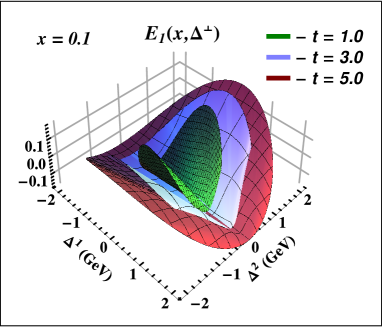
Figure 1: (Color online) Plots of $E_{1}(x,\Delta^{\perp})$ vs $\Delta^{1},\Delta^{2}$ for fixed values of $x$ and different $t$. $t$ is in ${\mathrm{GeV}}^{2}$. The innermost surface is for the smallest value of $-t$.

So we have;

$$E_{1}=\frac{\alpha e_{q}^{2}}{2\pi}x(1-x)^{3}({(\Delta^{1})}^{2}-{(\Delta^{2})}^{2})\Big{[}\int_{0}^{1}\frac{dq}{B(q)}\hskip 5.69046pt((1-q)^{2}-(1-q))\Big{]}.$$ (15)

The above has the expected quadrupole structure coming from $({(\Delta^{1})}^{2}-{(\Delta^{2})}^{2})$. As the photon is a spin one particle, in order to flip its helicity, the overlapping light-front wave functions should have a difference of orbital angular momentum of two units, which manifests itself in the quadrupole structure. This is in accordance with a similar observation for the helicity-flip GPD $E$ for the proton, which needs overlapping LFWFs of orbital angular momentum $\pm 1$ unit overlap ; spin .

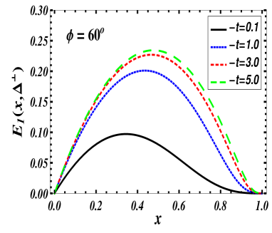
(a)    (b)

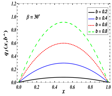
Figure 2: (Color online) Plots of (a) $E_{1}(x,\Delta^{\perp})$ vs $x$ for different values of $t$ in $\mathrm{GeV}^{2}$ and (b) $q_{1}(x,b^{\perp})$ vs. $x$ for different values of $b$ in $\mathrm{GeV}^{-1}$. $\phi={\mathrm{tan}}^{-1}{\Delta^{2}\over\Delta^{1}}$ and $\beta={\mathrm{tan}}^{-1}{b^{2}\over b^{1}}$.

From the off-forward matrix element $\tilde{F}_{q}$ we extract the GPDs that flip the helicity of the photon by calculating the coefficient of the combination $(\epsilon_{+1}^{1}\epsilon_{-1}^{2*}+\epsilon_{+1}^{2}\epsilon_{-1}^{1*})$ which gives:

$$\tilde{E_{1}}=\frac{\alpha e_{q}^{2}}{4\pi^{2}}(x-x^{\prime})\Big{[}\tilde{I}_{1}-(1-x^{\prime})\tilde{I}_{2}\Big{]}$$

$$\tilde{I}_{1}=\pi\int_{0}^{1}dq\hskip 5.69046pt\Big{(}(\Delta_{1}^{2}-\Delta_{2}^{2})\frac{(1-q)^{2}}{B(q)}(1-x^{\prime})^{2}\Big{)}$$

$$\tilde{I}_{2}=\pi\int_{0}^{1}dq\hskip 5.69046pt\hskip 5.69046pt(\Delta_{1}^{2}-\Delta_{2}^{2})\frac{(1-q)}{B(q)}(1-x^{\prime})$$

$$\tilde{E_{1}}=\frac{\alpha e_{q}^{2}}{2\pi}(x-x^{\prime})(1-x^{\prime})^{2}(\Delta_{1}^{2}-\Delta_{2}^{2})\Big{[}\int_{0}^{1}\frac{dq}{B(q)}\hskip 5.69046pt(-q)(1-q)\Big{]}$$ (16)

Here $x^{\prime}$ is the longitudinal momentum fracion of the quark in the final photon LFWF. As we have taken the momentum transfer to be purely in the transverse direction, $x^{\prime}=x$ and $\tilde{E}_{1}=0$. $E_{1}$ and $\tilde{E}_{1}$ are only two independent structures that cause helicity flip of the photon. Other helicity-flip GPDs that can be constructed from other combinations of the polarization vectors can be related to these by phase change in the $\Delta^{\perp}$ plane. However a proper counting of the photon GPD (both helicty non-flip and helicity flip) can only be done in a formal parametrization of Eqs. (1) and (2).

Like the GPD $E$ of a spin $1/2$ particle for example a dressed electron/quark quark , the helicity flip photon GPD has no logarithmic term depending on the hard scale of the process $Q^{2}$, which is the virtuality of the probing photon. Starting from the expressions of photon GPDs, we define the parton distributions burkardt with the helicity flip of the photon in transverse impact parameter space as:

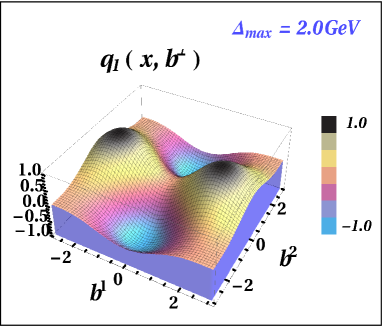
(a)    (b)

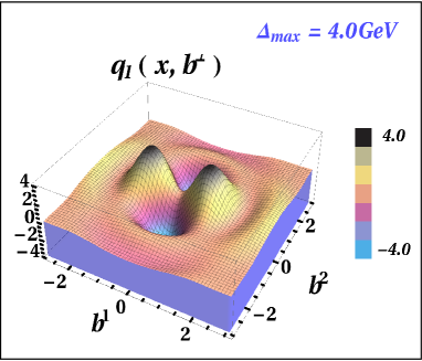
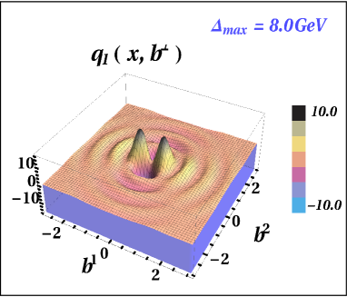
(c)    (d)

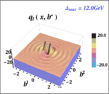
Figure 3: (Color online) Plots of $q_{1}(x,b^{\perp})$ vs. $b^{1},b^{2}$ for different values of $\Delta_{max}$. $b^{1}$ and $b^{2}$ are in $\mathrm{GeV}^{-1}$ and $\Delta_{max}$ is in GeV. $x=0.3$.

$$q_{1}(x,b^{\perp})={1\over 4\pi^{2}}\int d^{2}\Delta^{\perp}e^{-i\Delta^{\perp}\cdot b^{\perp}}E_{1}(x,\Delta^{\perp});$$ (17)

where $t=-{(\Delta^{\perp})}^{2}$ and $b^{\perp}$ is the transverse impact parameter conjugate to $\Delta^{\perp}$. One then gets

$$q_{1}(x,b^{\perp})=\frac{1}{4\pi^{2}}\int d^{2}\Delta^{\perp}e^{-ib^{\perp}\cdot\Delta^{\perp}}({(\Delta^{1})}^{2}-{(\Delta^{2})}^{2})f(x)Q(x,t),$$ (18)

where

$$f(x)=\frac{\alpha e_{q}^{2}}{2\pi}x(1-x)^{3}\hskip 14.22636pt,~{}~{}~{}~{}\hskip 14.22636ptQ(x,t)=\int_{0}^{1}\frac{dq}{B(q)}\hskip 5.69046pt((1-q)^{2}-(1-q));$$ (19)

This can be written as,

$$q_{1}(x,b^{\perp}) = \frac{1}{4\pi^{2}}\Big{(}\frac{\partial^{2}}{\partial{(b^{2})}^{2}}-\frac{\partial^{2}}{\partial{(b^{1})}^{2}}\Big{)}\int d^{2}\Delta^{\perp}e^{-ib^{\perp}\cdot\Delta^{\perp}}f(x)Q(x,t)$$ (20)

$$= \frac{1}{2\pi}\Big{(}\frac{\partial^{2}}{\partial{(b^{2})}^{2}}-\frac{\partial^{2}}{\partial{(b^{1})}^{2}}\Big{)}\Big{[}\int_{0}^{\infty}\Delta d\Delta\hskip 5.69046ptJ_{0}(b\Delta)\hskip 5.69046ptf(x)Q(x,t)\Big{]}.$$

Here $\Delta=\mid\Delta^{\perp}\mid$ and $b=\mid b\mid$. Using the integral representation for the Bessel function $J_{0}(x)$, the above can be written as,

$$q_{1}(x,b^{\perp})=\frac{1}{2\pi}\Big{(}\frac{\partial^{2}}{\partial{(b^{2})}^{2}}-\frac{\partial^{2}}{\partial{(b^{1})}^{2}}\Big{)}\Big{[}\int_{0}^{\infty}\Delta d\Delta\hskip 5.69046pt\frac{1}{\pi}\int_{0}^{\pi}\mathrm{cos}(b\Delta-\mathrm{\mathrm{sin}}\theta)d\theta\hskip 5.69046ptf(x)Q(x,t)\Big{]}.$$ (21)

We then get

$$q_{1}(x,b^{\perp})=\frac{1}{2\pi}\int_{0}^{\infty}\Delta d\Delta\hskip 5.69046pt\frac{1}{\pi}\int_{0}^{\pi}(P_{2}(b,\Delta,\theta)-P_{1}(b,\Delta,\theta))d\theta\hskip 5.69046ptf(x)Q(x,t);$$ (22)

where

$$P_{2}(b,\Delta,\theta)=-\frac{1}{b^{3}}\Delta\mathrm{sin}\theta\Big{[}{(b^{2})}^{2}b\Delta\mathrm{cos}\Big{(}b\Delta\mathrm{sin}\theta\Big{)}\mathrm{sin}\theta+$$ (23)

$${(b^{1})}^{2}\mathrm{sin}\Big{(}b\Delta\mathrm{sin}\theta\Big{)}\Big{]}$$

$$P_{1}(b,\Delta,\theta)=-\frac{1}{b^{3}}\Delta\mathrm{sin}\theta\Big{[}{(b^{1})}^{2}b\Delta\mathrm{cos}\Big{(}b\Delta\mathrm{sin}\theta\Big{)}\mathrm{sin}\theta+$$ (24)

$${(b^{2})}^{2}\mathrm{sin}\Big{(}b\Delta\mathrm{sin}\theta\Big{)}\Big{]}.$$

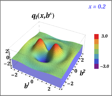
(a)    (b)

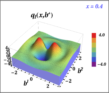
Figure 4: (Color online) Plots of $q_{1}(x,b^{\perp})$ vs $b^{1},b^{2}$ for different values of $x$ and at $\Delta_{max}=4.0$ GeV.

Numerical Results

We next discuss the numerical results. In Fig. 1, we have shown the helicity flip GPD of the photon as functions of $\Delta^{\perp}$. As we mentioned before, we took $\zeta=0$. In this kinematical limit, the GPDs are represented by overlaps of two-particle photon LFWFs. When $\zeta$ is non-zero or the momentum transfer between the initial to final photon has a longitudinal component, off-diagonal particle number changing overlaps of LFWFs has to be considered as well overlap . We take the mass of the quark and the antiquark in the photon to be the same and equal to 3.3 MeV. As seen in Eq. (9), the GPDs have two contributions. When $x$ is positive, the contribution comes from the active quark in the photon; and when $x$ is negative, the active antiquark contributes. In the numerical plots, we take $0<x<1$ and show the quark contribution. Fig. 1 shows the helicity flip GPD $E_{1}(x,\Delta^{\perp})$ as functions of $\Delta^{1}$ and $\Delta^{2}$ and for different values of $x$ for fixed values of $t$. $E_{1}(x,\Delta^{\perp})$ is zero when $\Delta^{1}=\Delta^{2}$. The curvature is sharper as $\mid t\mid$ decreases. As we already saw, $E_{1}(x,\Delta^{\perp})$ has a quadrupole structure in $\Delta^{\perp}$ plane coming from the ${(\Delta^{1})}^{2}-{(\Delta^{2})}^{2}$. Such quadrupole structure is due to the spin flip of a spin one particle and corresponds to an overlapping LFWF with two units of orbital angular momentum. The structure can be contrasted with the GPD $E(x,\Delta^{\perp})$ of a spin $1/2$ composite particle like a dressed electron or a proton quark ; model ; manohar2 . It is to be noted that the off-forward matrix element similar to Eq. (1) for a proton target is parametrized in terms of the GPDs $H$ and $E$. When the final proton has the same helicity as the initial proton, and $\zeta$ is non-zero, both the GPDs contribute. However when the helicity of the proton is flipped then only the GPD $E$ contributes. A parametrization of the off-forward matrix element for a spin one massive target like deuteron was given in one . So far no such parametrization is available for the photon GPDs and in this work as well as in two previous publications ours1 ; ours2 we calculate the full off-forward matrix element using overlaps of photon LFWFs. In Fig. 2(a) we have plotted the helicity flip photon GPD $E_{1}(x,\Delta^{\perp})$ vs. $x$ for different values of $t$ and a fixed value of $\phi=tan^{-1}{\Delta^{2}\over\Delta^{1}}$. As before, we have plotted for the region $0<x<1$, where the contribution to the GPD comes from the active quark. The peak of $E_{1}(x,\Delta^{\perp})$ increases as $-t$ increases and also shifts towards larger value of $x$. The GPD is zero both at $x=0$ and $x=1$. In fact, the GPD is zero when $\Delta^{\perp}=0$. This is because in order to flip the helicity one needs non-zero OAM in the two-particle LFWFs and the OAM is zero when there is no momentum transfer in the transverse direction. At $x=0$ and $x=1$ all momenta are carried by either the quark or the antiquark in the photon. Then there is no relative motion and no OAM contribution. In Fig. 2 (b) we have plotted the Fourier transform (FT) of the helicity-flip photon GPD, $q_{1}(x,b^{\perp})$ vs. $x$ for different $b=\mid b^{\perp}\mid$ at a fixed value of $\beta=tan^{-1}{b^{2}\over b^{1}}$. $q_{1}(x,b^{\perp})$ is symmetric with respect to $x=0$ and $x=1$ and maximum when $x=0.5$, that is when the quark and the antiquark carry equal momenta. As seen in Eq. (21), $q_{1}(x,b^{\perp})$ has a quadrupole structure, that comes because it involves a helicity flip of a spin one object (photon). This quadrupole structure is visible in the 3D plots of Figs 3 and 4. In the ideal definition of the Fourier transform, the limits of the $\Delta^{\perp}$ integration should be from $0$ to $\infty$. As we saw for the photon GPDs that do not involve a helicity flip ours1 ; ours2 , the $\Delta^{\perp}$ independent terms then give a $\delta(b^{\perp})$ in impact parameter space. For non-zero $\Delta^{\perp}$, we get a smearing in $b^{\perp}$. For the GPD with helicity flip, from Eq. (21), we see that it involves a distortion in $b^{\perp}$ space. The GPD as well as its FT is zero when $\Delta^{\perp}=0$, which means that it is purely an effect of the orbital angular momentum of the LFWF. In the actual numerical calculation we have imposed an upper limit on the $\Delta^{\perp}$ integration, denoted by $\Delta_{max}$. Fig. 3 shows a plot of $q_{1}(x,b^{\perp})$ vs. $b^{1}$ and $b^{2}$ for a fixed value of $x=0.3$ and different values of $\Delta_{max}$. It is seen that as $\Delta_{max}$ increases the peaks become sharper, which means that the distortion in $b^{\perp}$ space moves closer to the origin. Fig. 4 shows plots of $q_{1}(x,b^{\perp})$ vs. $b^{1}$ and $b^{2}$ for a fixed value of $\Delta_{max}$ and two different values of $x$. The magnitude of the peaks depend on $x$.

Conclusion

In this work we have calculated the GPDs of the photon when the helicity of the target photon is flipped. We expressed the GPDs in terms of overlaps of photon LFWFs. In the kinematics when the momentum transfer between the initial and the final photon is purely in the transverse direction, the GPDs involve diagonal overlaps of two-particle LFWFs at leading order in the electromagnetic coupling $\alpha$ and zeroth order in the strong coupling $\alpha_{s}$. Such two particle LFWFs of the photon can be calculated in light-front Hamiltonian perturbation theory. Taking a Fourier transform of the GPDs with respect to $\Delta^{\perp}$ we obtained impact parameter dependent parton distributions. Like the proton GPD $E$ the helicity flip GPD of the photon represents a distortion of the parton distribution in the impact parameter space. This is due to the orbital angular momentum contribution coming from the LFWFs. As photon is a spin one object, one needs OAM of two units in the overlapping LFWF to flip the helicity. The expected quadrupole structure is visible in impact parameter space. For the proton, such distortion in $b^{\perp}$ space has been found to be related to the Sivers function in some models. It will be interesting to check if such relations exist also for the photon. For this it is necessary to have a parametrization of the off-forward as well as the transverse momentum dependent matrix elements for the photon.

Acknowledgments

This work is supported by the DST project SR/S2/HEP-029/2010, Govt. of India. We thank B. Pire for suggesting this topic and for helpful discussions.

References

(1) For reviews on generalized parton distributions,
and DVCS, see M. Diehl,
Phys. Rept, 388, 41 (2003); A. V. Belitsky and A. V. Radyushkin, Phys.
Rept. 418 1, (2005); K. Goeke, M.
V. Polyakov, M. Vanderhaeghen, Prog. Part. Nucl. Phys. 47, 401 (2001).
(2) S. Friot, B. Pire, L. Szymanowski, Phys. Lett. B
645 153 (2007).
(3) T. F. Walsh and P. M. Zerwas, Phys. Lett. B 44, 95
(1974); E. Witten, Nucl. Phys. B 120, 189 (1977);
A. Buras, Acta. Phys. Polon. B 37, 683 (2006).
(4) M. El Beiyad, B. Pire, L. Szymanowski, S. Wallon,
Phys. Rev. D 78, 034009 (2008).
(5) A. Mukherjee, Sreeraj Nair, Phys. Lett. B
706 77 (2011).
(6) A. Mukherjee, Sreeraj Nair, Phys. Lett. B
707 99 (2012).
(7) I. R. Gabdrakhmanov, O. V. Teryaev, Phys. Lett. B 716,
417 (2012).
(8) M. Burkardt, Int. J. Mod. Phys. A 18, 173 (2003);
M. Burkardt, Phys. Rev. D 62, 071503 (2000), Erratum-
ibid, D 66, 119903 (2002); J. P. Ralston and B. Pire, Phys. Rev. D 66, 111501 (2002).
(9) W. M. Zhang, A. Harindranath, Phys. Rev. D48, 4881
(1993).
(10) S. J. Brodsky, M. Diehl, D. S. Hwang, Nucl. Phys. B
596, 99 (2001); M. Diehl, T. Feldman, R. Jakob, P. Kroll, Eur. Phys.
J. C 39, 1 (2005).
(11) A. Mukherjee, I. V. Musatov, H. C. Pauli, A. V. Radyushkin,
Phys. Rev. D 67, 073014 (2003).
(12) S. J. Brodsky, D. S. Hwang, B-Q. Ma, I. Schmidt, Nucl. Phys.
B 593, 311 (2001).
(13) D. Chakrabarti and A. Mukherjee,
Phys.Rev.D72, 034013 (2005);
Phys. Rev. D71, 014038 (2005).
(14) D. Chakrabarti, R. Manohar, A. Mukherjee,
Phys. Lett. B 682, 428 (2010);
(15) R. Manohar, A. Mukherjee, D.
Chakrabarti, Phys.Rev.D83, 014004,(2011).
(16) E. R. Berger, F. Cano, M. Diehl, B. Pire, Phys. Rev. Lett.
87, 142302 (2001).
(b)
(b)
(b)
(b)
(b)
(b)
(d)
(d)
(b)
(b)