General theory for interactions in sufficient cause models with dichotomous exposures

Abstract

The sufficient-component cause framework assumes the existence of sets of sufficient causes that bring about an event. For a binary outcome and an arbitrary number of binary causes any set of potential outcomes can be replicated by positing a set of sufficient causes; typically this representation is not unique. A sufficient cause interaction is said to be present if within all representations there exists a sufficient cause in which two or more particular causes are all present. A singular interaction is said to be present if for some subset of individuals there is a unique minimal sufficient cause. Empirical and counterfactual conditions are given for sufficient cause interactions and singular interactions between an arbitrary number of causes. Conditions are given for cases in which none, some or all of a given set of causes affect the outcome monotonically. The relations between these results, interactions in linear statistical models and Pearl’s probability of causation are discussed.

and t1Supported by the National Institutes of Health (R01 ES017876). t2Supported by NSF (CRI 0855230), the National Institutes of Health (R01 AI032475) and the Institute of Advanced Studies, University of Bologna.

1 Introduction

Rothman’s sufficient-component cause model Rothman1976 postulates a set of different causal mechanisms, each sufficient to bring about the outcome under consideration. Rothman refers to these hypothesized causal mechanisms as “sufficient causes,” conceiving of them as minimal sets of actions, events or states of nature which together initiate a process resulting in the outcome.

Thus each sufficient cause is hypothesized to consist of a set of “component causes.” Whenever all components of a particular sufficient cause are present, the outcome occurs; within every sufficient cause, each component would be necessary for that sufficient cause to lead to the outcome. Models of this kind have a long history: a simple version is considered by Cayley cayley1853 ; it also corresponds to the INUS model introduced by Mackie Mackie1965 in the philosophical literature; see also blisstoxicity1939 for an early application. Much recent work has sought to relate the model to other causal modeling frameworks Greenland2002 , Flanders2006 , VanderWeele2006 , VanderWeele2007a , VanderWeele2008a .

In traditional sufficient-component cause [SCC] models, the outcome and all the component causes are events, or equivalently, binary random variables. An SCC model with $k$ component causes implies a set of $2^{k}$ potential outcomes. Conversely, in Section 2 we show that for any given list of potential outcomes there is at least one SCC model which represents this set. However, in general there may be many such SCC models.

One question concerns whether, given a set of potential outcomes implied by some (unknown) SCC model, one may infer that two component causes are present within some sufficient cause in the unknown SCC model. In general, it is possible that two SCC models both imply the same set of potential outcomes, yet although $A$ and $B$ occur together in some sufficient component cause in the first model, $A$ and $B$ are not present together in any sufficient component cause in the second. In VanderWeele2008a two sufficient component causes are said to form a “sufficient cause interaction” (or to be “irreducible”) if they are both present within at least one sufficient cause in every SCC model for a given set of potential outcomes. Of course, in general, the distribution of potential outcomes for a given population is also unknown, though it is constrained (marginally) by the observed data from a randomized experiment. In VanderWeele2008a empirical conditions are given which are sufficient to ensure that for any set of potential outcomes compatible with experimental data, all compatible SCC models will contain a sufficient cause involving $A$ and $B$. These results were an improvement upon earlier empirical tests for the existence of a two-way interaction in an SCC model Rothman1998 , which required the assumption of monotonicity; see also Koopman1981 , Greenland1988 , Novick2004 , Aickin2002 , VanderWeele2007c . The new results are able to establish the existence of an interaction in situations where monotonicity does not hold. In this paper we develop empirical conditions that are sufficient for the existence of a sufficient cause containing a given subset of an arbitrary number of variables, both with and without monotonicity assumptions.

As illustrative motivation for the theoretical development, we will consider data presented in a study by Taylor1998 , summarized in Table 1, from a case-control study of bladder cancer examining possible three-way interaction between smoking ($1={}$present), and genetic variants on NAT2 ($0=R$, $1=S$ genotype) and NAT1 ($1$ for the *10 allele) for Caucasian individuals. We return to this example at the end of this paper to examine the evidence for a sufficient cause containing all three: smoking, the S genotype on NAT2 and the *10 allele on NAT1.

Table 1: Case-control data from a study of bladder cancer Taylor1998

			Cases	Controls
Smoking	NAT2	NAT1*10	$\bolds{(n=215)}$	$\bolds{(n=191)}$	Odds ratio (95% CI)
0	0	0	06	13	10000000000.
0	0	1	08	16	1.1 (0.3, 3.9)0
0	1	0	16	31	1.1 (0.4, 3.5)0
0	1	1	06	10	1.3 (0.3, 5.3)0
1	0	0	42	32	2.8 (1.1, 8.3)0
1	0	1	41	26	3.4 (1.2, 10.1)
1	1	0	61	51	2.6 (0.9, 7.3)0
1	1	1	35	12	6.3 (2.0, 20.3)

The remainder of this paper is organized as follows: Section 2 presents the sufficient-component cause framework as formalized by VanderWeele and Robins VanderWeele2008a . Section 3 describes general $n$-way irreducible interactions (aka “sufficient cause interactions”) and characterizes these in terms of potential outcomes. Section 4 derives empirical conditions for the existence of irreducible interactions both with and without monotonicity assumptions. Section 5 describes “singular” interactions which arise in genetic contexts, provides a characterization, derives empirical conditions that are sufficient for their existence and relates this notion to Pearl’s probability of causation. Section 6 discusses the relation between singular and sufficient cause interactions and linear statistical models. Section 7 provides some comments regarding stronger interpretations of sufficient cause models, and returns to the data presented in Table 1. Finally Section 8 offers some possible extensions to the present work.

2 Notation and basic concepts

We will use the following notation: An event is a binary random variable taking values in $\{0,1\}$. We use uppercase roman to indicate events ($X$), boldface to indicate sets of events ($\mathbf{C}$), and lowercase to indicate specific values both for single random variables ($X=x$), and, with slight abuse of notation, for sets $\{\mathbf{C=c}\}\equiv\{\forall i,(\mathbf{C})_{i}=(\mathbf{c})_{i}\}$ and $\{\mathbf{a\leq b}\}\equiv\{\forall i,(\mathbf{a})_{i}\leq(\mathbf{b})_{i}\}$; $\mathbf{1}$ and $\mathbf{0}$ are vectors of $1$’s and $0$’s; the cardinality of a set is denoted $|\mathbf{C}|$. We use fraktur (${\mathfrak{B}}$) to denote collections of sets of events.

The complement of some event $X$ is denoted by $\overline{X}\equiv 1-X$. A literal event associated with $X$, is either $X$ or $\overline{X}$. For a given set of events $\mathbf{C}$, $\mathbb{L}(\mathbf{C})$ is the associated set of literal events

$$\mathbb{L}(\mathbf{C})\equiv\mathbf{C}\cup\{\overline{X}|X\in\mathbf{C}\}.$$

For a literal $L\in\mathbb{L}(\mathbf{C})$, and an assignment $\mathbf{c}$ to $\mathbf{C}$, $(L)_{\mathbf{c}}$ denotes the value assigned to $L$ by $\mathbf{c}$. The conjunction of a set of literal events $\mathbf{B}=\{F_{1},\ldots,F_{m}\}\subseteq\mathbb{L}(\mathbf{C})$ is defined as

$$\bigwedge(\mathbf{B})\equiv\prod_{i=1}^{m}F_{i}=\min\{F_{1},\ldots,F_{m}\};$$

note that $\bigwedge(\mathbf{B})=1$ if and only if for all $i$, $F_{i}=1$. We also define $B_{1}\wedge B_{2}\equiv\bigwedge\{B_{1},B_{2}\}$. We will use ${\mathbb{I}}(A)$ to denote the indicator function for event $A$. There is a simple correspondence between conjunctions of literals and indicator functions: let $\mathbf{B}=\{X_{1},\ldots,X_{s}\}$ and $\mathbf{C}=\{Y_{1},\ldots,Y_{t}\}$, then

$$\bigwedge\bigl{(}\{X_{1},\ldots,X_{s},\overline{Y}_{1},\ldots,\overline{Y}_{t}\}\bigr{)}=1\quad\Leftrightarrow\quad{\mathbb{I}}\bigl{(}\{\mathbf{B}=\mathbf{1},\mathbf{C}=\mathbf{0}\}\bigr{)}=1.$$ (1)

Similarly, the set of literals corresponding to an assignment $\mathbf{c}$ to $\mathbf{C}$ is defined

$$\mathbf{B}^{[\mathbf{c}]}\equiv\bigl{\{}L|L\in{\mathbb{L}}(\mathbf{C}),(L)_{\mathbf{c}}=1\bigr{\}}$$

so that $\bigwedge(\mathbf{B}^{[\mathbf{c}]})={\mathbb{I}}(\mathbf{C}=\mathbf{c})$; note that $|\mathbf{B}^{[\mathbf{c}]}|=|\mathbf{C}|$. The disjunction of a set of binary random variables is defined as

$$\bigvee\bigl{(}\{Z_{1},\ldots,Z_{p}\}\bigr{)}\equiv\max\{Z_{1},\ldots,Z_{p}\};$$

note that $\bigvee(\{Z_{1},\ldots,Z_{p}\})=1$ if and only if for some $j$, $Z_{j}=1$. Similarly we let $B_{1}\vee B_{2}\equiv\bigvee\{B_{1},B_{2}\}$. Given a collection of sets of literals ${\mathfrak{B}}=\{\mathbf{C}_{1},\ldots,\mathbf{C}_{q}\}$, we define

$$\bigvee\bigwedge({\mathfrak{B}})\equiv\bigvee_{i}\Bigl{(}\bigwedge(\mathbf{C}_{i})\Bigr{)}.$$

We use $\dot{\mathbb{P}}(\mathbb{L}(\mathbf{C}))$ to denote the set of subsets of $\mathbb{L}(\mathbf{C})$ that do not contain both $X$ and $\overline{X}$ for any $X\in\mathbf{C}$; more formally,

$$\dot{\mathbb{P}}\bigl{(}\mathbb{L}(\mathbf{C})\bigr{)}\equiv\bigl{\{}\mathbf{B}|\mathbf{B}\subset\mathbb{L}(\mathbf{C})\mbox{ for all }X\in\mathbf{C},\{X,\overline{X}\}\nsubseteq\mathbf{B}\bigr{\}}.$$

Note that if $\mathbf{B}\in\dot{\mathbb{P}}(\mathbb{L}(\mathbf{C}))$, and $|\mathbf{B}|=|\mathbf{C}|$, so that for all $C\in\mathbf{C}$, exactly one of $C$ or $\overline{C}$ is in $\mathbf{B}$, then an assignment of values $\mathbf{b}$ to $\mathbf{B}$ induces a unique assignment $\mathbf{c}$ to $\mathbf{C}$ and vice versa.

2.1 Potential outcomes models

Consider a potential outcome model Neyman1923 , Rubin1974 , Rubin1978 with $s$ binary factors, $X_{1},\ldots,X_{s}$, which represent hypothetical interventions or causes, and let $D$ denote some binary outcome of interest. We use $\Omega$ to denote the sample space of individuals in the population and use $\omega$ for a particular sample point. Let $D_{x_{1},\ldots,x_{s}}(\omega)$ denote the counterfactual value of $D$ for individual $\omega$ if the cause $X_{j}$ were set to the value $x_{j}$ for $j=1,\ldots,s$. The potential outcomes framework we employ makes two assumptions: first, that for a given individual these counterfactual variables are deterministic; second, in asserting that the counterfactual $D_{x_{1},\ldots,x_{s}}(\omega)$ is well defined, it is implicitly assumed that the value that $D$ would take on for individual $\omega$ is determined solely by the values that $X_{1},\ldots,X_{s}$ are assigned for this individual, and not the assignments made to these variables for other individuals $\omega^{\prime}$. This latter assumption is often called “no interference” Cox1958 , or the stable unit treatment value assumption (SUTVA) Rubin1990 . An example of a situation where this assumption might fail is a vaccine trial where there is “herd” immunity.

We will use $D_{x_{1},\ldots,x_{s}}(\omega)$, $D_{X_{1}=x_{1},\ldots,X_{s}=x_{s}}(\omega)$, $D_{\mathbf{c}}$ and $D_{\mathbf{C=c}}(\omega)$, with $\mathbf{C}=\{X_{1},\ldots,X_{s}\}$ interchangeably. In this setting there will be $2^{s}$ potential outcomes for each individual $\omega$ in the population, one potential outcome for each possible value of $(X_{1},\ldots,X_{s})$; we use ${\mathcal{D}}(\mathbf{C};\omega)$ to denote the set of all such potential outcomes for an individual, and ${\mathcal{D}}(\mathbf{C};\Omega)$ for the population. Note that if $G=g(\mathbf{C})$ is some deterministic function of $\mathbf{C}$, then $G_{\mathbf{C=c}}(\omega)=g(\mathbf{c)}$, and hence is constant; thus our usage is consistent with the definition of $(L)_{\mathbf{c}}$ in the previous section.

Table 2: All potential outcomes and actual outcomes for three binary causes, $X_{1}$, $X_{2}$ and $X_{3}$, in a population with two individuals

Individual	$\bolds{D_{000}}$	$\bolds{D_{001}}$	$\bolds{D_{010}}$	$\bolds{D_{011}}$	$\bolds{D_{100}}$	$\bolds{D_{101}}$	$\bolds{D_{110}}$	$\bolds{D_{111}}$	$\bolds{(X_{1},X_{2},X_{3})}$	$\bolds{D}$
1	0	1	1	0	0	1	1	0	$(1,0,1)$	1
2	0	1	1	0	0	1	1	1	$(0,0,0)$	0

The actual observed value of $D$ for individual $\omega$ will be denoted by $D(\omega)$ and similarly the actual value of $X_{1},\ldots,X_{s}$ by $X_{1}(\omega),\ldots,X_{s}(\omega)$. Actual and counterfactual outcomes are linked by the consistency axiom which requires that

$$D_{X_{1}=X_{1}(\omega),\ldots,X_{s}=X_{s}(\omega)}(\omega)=D(\omega),$$ (2)

that is, that the value of $D$ which would have been observed if $X_{1},\ldots,X_{s}$ had been set to the values they actually took is equal to the value of $D$ which was in fact observed Robins1986 . It follows from this axiom that $D_{X_{1}(\omega),\ldots,X_{s}(\omega)}(\omega)=D$ is observed, but it is the only potential outcome for individual $\omega$ that is observed.

Example 1.

Consider a binary outcome $D$ with three binary causes of interest, $X_{1}$, $X_{2}$ and $X_{3}$. Suppose that the population consists of two individuals. The potential outcomes (left-hand side) and actual outcomes (right-hand side) are shown in Table 2.

We use the notation $A\perp\!\!\!\perp B|C$ to indicate that $A$ is independent of $B$, conditional on $C$ in the population distribution.

2.2 Definitions for sufficient cause models

The following definitions generalize those in VanderWeele2008a to sub-populations, $\varnothing\neq\Omega^{*}\subseteq\Omega$:

Definition 2.1 ((Sufficient cause)).

A subset $\mathbf{B}$ of the putative (binary) causes ${\mathbb{L}}(\mathbf{C})$ for $D$ forms a sufficient cause for $D$ (relative to $\mathbf{C}$) in sub-population $\Omega^{*}$ if for all $\mathbf{c}\in\{0,1\}^{|\mathbf{C}|}$ such that $(\bigwedge(\mathbf{B}))_{\mathbf{c}}=1$, $D_{\mathbf{c}}(\omega)=1$ for all $\omega\in\Omega^{*}\subseteq\Omega$. [We require that there exists a $\mathbf{c}^{*}$ such that $(\bigwedge(\mathbf{B}))_{\mathbf{c^{*}}}=1$.]

Observe that if $\mathbf{B}$ is a sufficient cause for $D$, then any intervention setting the variables $\mathbf{C}$ to $\mathbf{c}$ with $(\bigwedge(\mathbf{B}))_{\mathbf{c}}=1$ will ensure that $D_{\mathbf{c}}(\omega)=1$ for all $\omega\in\Omega^{*}$. We restrict the definition to nonempty sets $\Omega^{*}$, to preclude every set $\mathbf{B}$ being a sufficient cause in an empty sub-population. Likewise we require that there exists some $\mathbf{c}^{*}$ such that $(\bigwedge(\mathbf{B}))_{\mathbf{c^{*}}}=1$ in order to avoid logically inconsistent conjunctions, for example, $X_{1}\wedge\overline{X}_{1}$, being classified (vacuously) as a sufficient cause. As a direct consequence, for any binary random variable $X$, at most one of $X$ and $\overline{X}$ appear in any sufficient cause $\mathbf{B}$.

Proposition 2.2.

In $\Omega^{*}$ if $\mathbf{B}$ is a sufficient cause for $D$ relative to $\mathbf{C}$, then $\mathbf{B}$ is sufficient for $D$ in any set $\mathbf{C}^{*}$ with $\mathbf{B}\subseteq\mathbf{C}^{*}\subseteq\mathbf{C}$.

$\mathbf{B}$ may be sufficient for $D$ relative to $\mathbf{C}$ in $\Omega^{*}$, but not relative to $\mathbf{C}^{\prime}\supset\mathbf{C}$.

Proposition 2.3.

If $\mathbf{B}$ is a sufficient cause for $D$ relative to $\mathbf{C}$ in $\Omega^{*}$, then $\mathbf{B}$ is sufficient for $D$ relative to $\mathbf{C}$ in any subset $\varnothing\neq\Omega^{**}\subseteq\Omega^{*}$.

$\mathbf{B}$ may be sufficient for $D$ relative to $\mathbf{C}$ in $\Omega^{*}$, but not in $\Omega^{\prime}\supset\Omega^{*}$.

Definition 2.4 ((Minimal sufficient cause)).

A set $\mathbf{B}\subset{\mathbb{L}}(\mathbf{C})$ forms a minimal sufficient cause for $D$ (relative to $\mathbf{C}$) in sub-population $\Omega^{*}$ if $\mathbf{B}$ constitutes a sufficient cause for $D$ in $\Omega^{*}$, but no proper subset $\mathbf{B}^{*}\subset\mathbf{B}$ also forms a sufficient cause for $D$ in $\Omega^{*}$.

Note that (in some $\Omega^{*}$) $\mathbf{B}$ may be a minimal sufficient cause for $D$ relative to $\mathbf{C}$, but not relative to $\mathbf{C}^{*}\subset\mathbf{C}$, so the analog of Proposition 2.2 does not hold. For individual $2$ in Table 2 $\{{X}_{1},{X}_{3}\}$ is a minimal sufficient cause relative to $\{X_{1},X_{2},X_{3}\}$. However, if we suppose that for $\omega=2$, $X_{2}$ is not caused by $X_{1}$ and $X_{3}$, so for all $x_{1}$, $x_{3}$, $X_{2X_{1}=x_{1},X_{3}=x_{3}}(\omega=2)=X_{2}(\omega=2)$, then $\{{X}_{1},{X}_{3}\}$ is not a minimal sufficient cause relative to $\{X_{1},X_{3}\}$.

$$D_{X_{1}=0,X_{3}=1}(\omega=2) = D_{X_{1}=0,X_{2}=0,X_{3}=1}(\omega=2)=1,$$

$$D_{X_{1}=1,X_{3}=1}(\omega=2) = D_{X_{1}=1,X_{2}=0,X_{3}=1}(\omega=2)=1$$

[since $X_{2}(\omega=2)=0$]; hence $X_{3}$ is a sufficient cause of $D$ relative to $\{X_{1},X_{3}\}$; hence $\{X_{1},{X}_{3}\}$ is not minimal relative to $\{X_{1},X_{3}\}$ for $\omega=2$.

Similarly, if $\mathbf{B}$ is a minimal sufficient cause for $D$ relative to $\mathbf{C}$ in $\Omega^{*}$, it does not follow that $\mathbf{B}$ is a minimal sufficient cause for $D$ relative to $\mathbf{C}$ in subsets $\Omega^{**}\subseteq\Omega^{*}$, so the analog to Proposition 2.3 does not hold. In particular, it may be the case that for all $\omega\in\Omega^{*}$, $\mathbf{B}$ is not a minimal sufficient cause for $D$ in $\{\omega\}$.

In the language of digital circuit theory marcovitz2001 , sufficient causes are termed “implicants,” and minimal sufficient causes are “prime implicants.”

Definition 2.5 ((Determinative set of sufficient causes)).

A set of sufficient causes for $D$, ${\mathfrak{B}}=\{\mathbf{B}_{1},\ldots,\mathbf{B}_{n}\}\subseteq\dot{\mathbb{P}}({\mathbb{L}}(\mathbf{C}))$, is said to be determinative for $D$ (relative to $\mathbf{C}$) in sub-population $\Omega^{*}$ if for all $\omega\in\Omega^{*}$ and for all $\mathbf{c}$, $D_{\mathbf{c}}(\omega)=1$ if and only if $(\bigvee\bigwedge({\mathfrak{B}}))_{\mathbf{c}}=1$.

We will refer to a determinative set of sufficient causes for $D$ as a sufficient cause model. Observe that in any sub-population $\Omega^{*}$ for which there exists a determinative set of sufficient causes, the vectors of potential outcomes for $D$ are identical, so ${\mathcal{D}}(\mathbf{C},\omega)={\mathcal{D}}(\mathbf{C},\omega^{\prime})$ for all $\omega,\omega^{\prime}\in\Omega^{*}$.

Definition 2.6 ((Nonredundant set of sufficient causes)).

A determinative set of sufficient causes ${\mathfrak{B}}$, for $D$, is said to be nonredundant (in $\Omega^{*}$, relative to C) if there is no proper subset ${\mathfrak{B}}^{*}\subset{\mathfrak{B}}$ that is also determinative for $D$.

Note that sufficient causes are conjunctions, while sets of sufficient causes form disjunctions of conjunctions; minimality refers to the components in a particular conjunction, that each component is required for the conjunction to be sufficient for $D$; nonredundancy implies that each conjunction is required for the disjunction of the set of conjunctions to be determinative. If for some set of sufficient causes $\mathfrak{B}\subseteq\dot{\mathbb{P}}(\mathbb{L}(\mathbf{C}))$, for all $X\in\mathbf{C}$, and all $\mathbf{B}\in\mathfrak{B}$, either $X\in\mathbf{B}$ or $\overline{X}\in\mathbf{B}$, then $\mathfrak{B}$ is a nonredundant set of sufficient causes.

Example 1 ((Revisited)).

The set $\mathfrak{B}_{1}=\{\{X_{1},X_{2}\},\{X_{2},\overline{X}_{3}\},\{\overline{X}_{2},X_{3}\}\}$ forms a determinative set of sufficient causes for the individual $\omega=2$, since

$$D_{\mathbf{c}}(\omega=2)=\bigl{(}(X_{1}\wedge X_{2})\vee(X_{2}\wedge\overline{X}_{3})\vee(\overline{X}_{2}\wedge X_{3})\bigr{)}_{\mathbf{c}}$$ (3)

as does $\mathfrak{B}_{2}=\{\{X_{1},X_{3}\},\{X_{2},\overline{X}_{3}\},\{\overline{X}_{2},X_{3}\}\}$:

$$D_{\mathbf{c}}(\omega=2)=\bigl{(}(X_{1}\wedge X_{3})\vee(X_{2}\wedge\overline{X}_{3})\vee(\overline{X}_{2}\wedge X_{3})\bigr{)}_{\mathbf{c}}.$$ (4)

As this example shows, determinative sets of sufficient causes are not, in general, unique.

2.3 Sufficient cause representations for a population

As noted, if $\mathbf{B}$ is a sufficient cause for $D$ in $\Omega^{*}$, then all the units in $\Omega^{*}$ will have $D=1$ for any assignment $\mathbf{c}$ to $\mathbf{C}$, such that $(\bigwedge(\mathbf{B}))_{\mathbf{c}}=1$. In most realistic settings it is unlikely that any set $\mathbf{B}$ will be sufficient to ensure $D=1$ in an entire population. Consequently, different sets of sufficient causes will be required within different sub-populations. A sufficient cause representation is a set of sub-populations, each with its own determinative sufficient cause representation.

Definition 2.7.

A sufficient cause representation $(\mathbf{A},{\mathfrak{B}})$ for ${\mathcal{D}}(\mathbf{C};\Omega)$ is an ordered set $\mathbf{A}=\langle A_{1},\ldots,A_{p}\rangle$ of binary random variables, with $(A_{i})_{\mathbf{c}}=A_{i}$ for all $i,\mathbf{c}$, and a set ${\mathfrak{B}}=\langle\mathbf{B}_{1},\ldots,\mathbf{B}_{p}\rangle$, with $\mathbf{B}_{i}\in\dot{\mathbb{P}}(\mathbb{L}(\mathbf{C}))$, such that for all $\omega$, $\mathbf{c}$, $D_{\mathbf{c}}(\omega)=1\Leftrightarrow\mbox{ for some }j,A_{j}(\omega)=1\mbox{ and }(\bigwedge(\mathbf{B}_{j}))_{\mathbf{c}}=1$.

Note that the binary random variables $A_{i}$ and the sets $\mathbf{B}_{i}$ are naturally paired via the orderings of $\mathbf{A}$ and ${\mathfrak{B}}$; we will refer to a pair $(A_{i},\mathbf{B}_{i})$ as occurring in the representation. The requirement that $(A_{i})_{\mathbf{c}}=A_{i}$ for all $i,\mathbf{c}$ implies that $\mathbf{A}\cap\mathbf{C}=\varnothing$, and further that the $A_{i}$ are unaffected by interventions on the $X_{i}$; this is in keeping with the interpretation of the $A_{i}$ as defining pre-existing sub-populations with particular sets of potential outcomes for $D$.

Proposition 2.8.

If $(\mathbf{A},{\mathfrak{B}})$ is a sufficient cause representation for ${\mathcal{D}}(\mathbf{C};\Omega)$, then $\mathbf{B}_{i}$ is a sufficient cause of $D$ in the sub-population in which $A_{i}(\omega)=1$.

Proposition 2.9.

If $(\mathbf{A},{\mathfrak{B}})$ is a sufficient cause representation for ${\mathcal{D}}(\mathbf{C};\Omega)$, then for all $\mathbf{A}^{*}\subseteq\mathbf{A}$, if

$$\varnothing\neq\Omega^{\mathbf{A}^{*}}_{\mathbf{A}\setminus\mathbf{A}^{*}}\equiv\bigl{\{}\omega|\mbox{ for all }A_{i}\in\mathbf{A},A_{i}(\omega)=1\mbox{ iff }A_{i}\in\mathbf{A}^{*}\bigr{\}},$$

then

$${\mathfrak{B}}^{\mathbf{A}^{*}}\equiv\bigl{\{}\mathbf{B}_{i}|\mathbf{B}_{i}\in{\mathfrak{B}};A_{i}\in\mathbf{A^{*}}\bigr{\}}$$

forms a determinative set of sufficient causes (relative to $\mathbf{C}$) for $\Omega^{\mathbf{A}^{*}}_{\mathbf{A}\setminus\mathbf{A}^{*}}$.

Note that $\Omega^{\mathbf{A}^{*}}_{\mathbf{A}\setminus\mathbf{A}^{*}}$ consists of the sub-population in which $A_{i}(\omega)=1$ for all $A_{i}\in\mathbf{A}^{*}$ and $A_{j}(\omega)=0$ for all $A_{j}\in\mathbf{A}\setminus\mathbf{A}^{*}$.

Suppose for some $\omega\in\Omega^{\mathbf{A}^{*}}_{\mathbf{A}\setminus\mathbf{A}^{*}}$, $\mathbf{B}_{j}\in{\mathfrak{B}}^{\mathbf{A}^{*}}$, and $\mathbf{c}$ we have$(\bigwedge(\mathbf{B}_{j}))_{\mathbf{c}}=1$. Since $\omega\in\Omega^{\mathbf{A}^{*}}_{\mathbf{A}\setminus\mathbf{A}^{*}}$, $A_{j}(\omega)=1$. It then follows from the definition of a sufficient cause representation that $D_{\mathbf{c}}(\omega)=1$. Conversely, suppose $D_{\mathbf{c}}(\omega)=1$. As $(\mathbf{A},{\mathfrak{B}})$ is a sufficient cause representation, for some $j$, $A_{j}(\omega)=1$ and $(\bigwedge(\mathbf{B}_{j}))_{\mathbf{c}}=1$. Since, by hypothesis, $\omega\in\Omega^{\mathbf{A}^{*}}_{\mathbf{A}\setminus\mathbf{A}^{*}}$, it follows that $A_{j}\in\mathbf{A}^{*}$, hence $\mathbf{B}_{j}\in{\mathfrak{B}}^{\mathbf{A}^{*}}$.

Theorem 2.10

For any ${\mathcal{D}}(\mathbf{C};\Omega)$, there exists a sufficient cause representation $(\mathbf{A},{\mathfrak{B}})$.

Let $p=2^{|\mathbf{C}|}$, and define ${\mathfrak{B}}\equiv\{\mathbf{B}|\mathbf{B}\subseteq\dot{\mathbb{P}}({\mathbb{L}}(\mathbf{C})),|\mathbf{B}|=|\mathbf{C}|\}\equiv\langle\mathbf{B}_{1},\ldots,\mathbf{B}_{p}\rangle$, ordered arbitrarily. Further define $A_{i}(\omega)\equiv D_{\mathbf{B}_{i}=\mathbf{1}}(\omega)$. Given an arbitrary $\mathbf{c}$, for some $j$, $\mathbf{B}^{[\mathbf{c}]}=\mathbf{B}_{j}$, by construction of ${\mathfrak{B}}$. We then have

$$D_{\mathbf{c}}(\omega)=1\quad\Leftrightarrow\quad D_{\mathbf{B}_{j}=\mathbf{1}}(\omega)=1\quad\Leftrightarrow\quad A_{j}(\omega)=1\quad\mbox{and}\quad\Bigl{(}\bigwedge(\mathbf{B}_{j})\Bigr{)}_{\mathbf{c}}=1$$

as required. The last step follows since by definition $\mathbf{B}^{[\mathbf{c}]}=\mathbf{1}$ if and only if $\mathbf{C}=\mathbf{c}$.

VanderWeele2008a prove this for the case of $|\mathbf{C}|=2$; see also Flanders2006 and VanderWeele2006 for discussion of the case $|\mathbf{C}|=1$.

Example 1 ((Revisited)).

The construction given in the proof of Theorem 2.10 would yield the following sets of sufficient causes to represent ${\mathcal{D}}(\mathbf{C};\Omega)$ shown in Table 2:

$${\mathfrak{B}} = \langle\mathbf{B}_{1},\ldots,\mathbf{B}_{8}\rangle$$

$$= \bigl{\langle}\{X_{1},X_{2},X_{3}\},\{X_{1},X_{2},\overline{X}_{3}\},\{X_{1},\overline{X}_{2},X_{3}\},\{X_{1},\overline{X}_{2},\overline{X}_{3}\},$$

$$\hskip 6.0pt\{\overline{X}_{1},X_{2},X_{3}\},\{\overline{X}_{1},X_{2},\overline{X}_{3}\},\{\overline{X}_{1},\overline{X}_{2},X_{3}\},\{\overline{X}_{1},\overline{X}_{2},\overline{X}_{3}\}\bigr{\rangle}$$

$\mbox{with }A_{1}={\mathbb{I}}\bigl{(}\{\omega=2\}\bigr{)},A_{4}=A_{5}=A_{8}=0,A_{2}=A_{3}=A_{6}=A_{7}=1.$

3 Irreducible conjunctions

We saw in Example 1 above with $\omega=2$ that an individual’s potential outcomes may be such that there are two determinative sets of common causes $\mathfrak{B}$ and $\mathfrak{B}^{\prime}$ and $\{X_{1},X_{2}\}$ is in $\mathfrak{B}$, but not in $\mathfrak{B}^{\prime}$. However, certain conjunctions are such that in every representation either the conjunction is present or it is contained in some larger conjunction; such conjunctions are said to be “irreducible.”

Definition 3.1.

$\mathbf{B}\in\dot{\mathbb{P}}({\mathbb{L}}(\mathbf{C}))$ is said to be irreducible for ${\mathcal{D}}(\mathbf{C},\Omega)$ if in every representation $(\mathbf{A},{\mathfrak{B}})$ for ${\mathcal{D}}(\mathbf{C},\Omega)$, there exists $\mathbf{B}_{i}\in{\mathfrak{B}}$, with $\mathbf{B}\subseteq\mathbf{B}_{i}$.

VanderWeele2008a also refer to irreducibility of $\mathbf{B}$ for ${\mathcal{D}}(\mathbf{C},\Omega)$ as a “sufficient cause interaction” between the components of $\mathbf{B}$. (Note, however, that if $\mathbf{B}$ is irreducible, this does not, in general, imply that $\mathbf{B}$ is either a minimal sufficient cause, or even a sufficient cause, only that there is a sufficient cause that contains $\mathbf{B}$.) It can be shown (via Theorem 3.2 below) that $\{X_{2},\overline{X}_{3}\}$ and $\{\overline{X}_{2},X_{3}\}$ are irreducible for ${\mathcal{D}}(\mathbf{C};\Omega)$ in Table 2. In Section 7 we provide an interpretation of irreducibility in terms of the existence of a mechanism involving the variables in $\mathbf{B}$. Using $\mathbf{C}_{1}\,\dot{\cup}\,\mathbf{C}_{2}$ to indicate the disjoint union of $\mathbf{C}_{1}$ and $\mathbf{C}_{2}$, we now characterize irreducibility:

Theorem 3.2

Let $\mathbf{C}=\mathbf{C}_{1}\,\dot{\cup}\,\mathbf{C}_{2}$, $\mathbf{B}\in\dot{\mathbb{P}}({\mathbb{L}}(\mathbf{C}_{1}))$, $|\mathbf{B}|=|\mathbf{C}_{1}|$.Then $\mathbf{B}$ is irreducible for ${\mathcal{D}}(\mathbf{C},\Omega)$ if and only if there exists $\omega^{*}\in\Omega$ and values $\mathbf{c}^{*}_{2}$ for $\mathbf{C}_{2}$ such that: (i) $D_{\mathbf{B}=\mathbf{1},\mathbf{C}_{2}=\mathbf{c}_{2}^{*}}(\omega^{*})=1$; (ii) for all $L\in\mathbf{B}$,$D_{\mathbf{B}\setminus\{L\}=\mathbf{1},L=0,\mathbf{C}_{2}=\mathbf{c}_{2}^{*}}(\omega^{*})=0$.

Thus $\mathbf{B}$ is irreducible if and only if there exists an individual in $\Omega$ who would have response $D=1$ if every literal in $\mathbf{B}$ is set to $1$, but $D=0$ whenever one literal is set to $0$ and the rest to $1$ (in some context $\mathbf{C}_{2}=\mathbf{c}_{2}^{\ast}$). Note that conditions (i) and (ii) are equivalent to

$$D_{\mathbf{B}=\mathbf{1},\mathbf{C}_{2}=\mathbf{c}_{2}^{\ast}}\bigl{(}\omega^{\ast}\bigr{)}-\sum_{L\in\mathbf{B}}D_{\mathbf{B}\setminus\{L\}=\mathbf{1},L=0,\mathbf{C}_{2}=\mathbf{c}_{2}^{\ast}}\bigl{(}\omega^{\ast}\bigr{)}>0.$$ (6)

($\Rightarrow$) We adapt the proof of Theorem 2.10 to show that if for all $\omega\in\Omega$ and assignments $\mathbf{c}_{2}^{*}$ to $\mathbf{C}_{2}$, at least one of (i) or (ii) does not hold, then there exists a representation $(\mathbf{A},{\mathfrak{B}})$ for ${\mathcal{D}}(\mathbf{C},\Omega)$ such that for all $\mathbf{B}_{i}\in{\mathfrak{B}}$, $\mathbf{B}\nsubseteq\mathbf{B}_{i}$. Define

$${\mathfrak{B}}^{{\dagger}} \equiv \bigl{\langle}\mathbf{B}^{\dagger}_{i}\bigr{\rangle}\equiv\bigl{\{}\mathbf{B}^{*}|\mathbf{B}^{*}\in\dot{\mathbb{P}}\bigl{(}{\mathbb{L}}(\mathbf{C})\bigr{)},|\mathbf{B}^{*}|=|\mathbf{C}|,\mathbf{B}\nsubseteq\mathbf{B}^{*}\bigr{\}},$$

$${\mathfrak{B}}^{{\ddagger}} \equiv \bigl{\langle}\mathbf{B}^{\ddagger}_{i}\bigr{\rangle}\equiv\bigl{\{}\mathbf{B}^{*}|\mathbf{B}^{*}\in\dot{\mathbb{P}}\bigl{(}{\mathbb{L}}(\mathbf{C})\bigr{)},|\mathbf{B}^{*}|=|\mathbf{C}|-1,\mathbf{B}\setminus\mathbf{B}^{*}=\{L\},L\in\mathbf{B}\bigr{\}},$$

under arbitrary orderings. Thus ${\mathfrak{B}}^{{\dagger}}$ is the set of subsets of exactly $|\mathbf{C}|$ literals that do not include $\mathbf{B}$ as a subset, while ${\mathfrak{B}}^{{\ddagger}}$ contains those subsets of size $|\mathbf{C}|-1$ that contain all but one literals in $\mathbf{B}$.

[]

For $\mathbf{B}^{\dagger}_{i}\in{\mathfrak{B}}^{{\dagger}}$ define the corresponding $A^{\dagger}_{i}(\omega)\equiv D_{\mathbf{B}^{\dagger}_{i}=\mathbf{1}}(\omega)$;

For $\mathbf{B}^{\ddagger}_{i}\in{\mathfrak{B}}^{{\ddagger}}$ define $A^{\ddagger}_{i}(\omega)\equiv D_{\mathbf{B}^{\ddagger}_{i}=\mathbf{1},L_{i}=0}(\omega)D_{\mathbf{B}^{\ddagger}_{i}=\mathbf{1},L_{i}=1}(\omega)$, where$\{L_{i}\}\equiv\mathbf{B}\setminus\mathbf{B}^{\ddagger}_{i}$.

The representation is given by $(\mathbf{A},{\mathfrak{B}})\equiv(\mathbf{A}^{\dagger}\cup\mathbf{A}^{{\ddagger}},{\mathfrak{B}}^{{\dagger}}\cup{\mathfrak{B}}^{{\ddagger}})$, where $\mathbf{A}^{\dagger}\equiv\langle A_{i}^{\dagger}\rangle$, $\mathbf{A}^{\ddagger}\equiv\langle A_{i}^{\ddagger}\rangle$. To see this, first note that if for some $\omega$ and $\mathbf{c}$, there is a pair $(A_{j},\mathbf{B}_{j})$ in $(\mathbf{A},{\mathfrak{B}})$ such that $A_{j}(\omega)=1$ and $(\bigwedge(\mathbf{B}_{j}))_{\mathbf{c}}=1$. Then by construction of $\mathbf{A}^{\dagger}$ and $\mathbf{A}^{{\ddagger}}$ it follows that $D_{\mathbf{c}}(\omega)=1$. For the converse, suppose that for some $\mathbf{c}$ and $\omega$, $D_{\mathbf{c}}(\omega)=1$. There are two cases to consider:

In this case $\mathbf{B}\nsubseteq\mathbf{B}^{[\mathbf{c}]}$, so for some $j$, $\mathbf{B}^{\dagger}_{j}=\mathbf{B}^{[\mathbf{c}]}$, hence $A_{j}^{\dagger}(\omega)\equiv D_{\mathbf{B}^{\dagger}_{j}=\mathbf{1}}(\omega)=D_{\mathbf{c}}(\omega)=1$, as required.

Let $\mathbf{c}$ be partitioned as $(\mathbf{c}_{1},\mathbf{c}_{2})$. Since (i) holds with $\mathbf{c}_{2}^{*}=\mathbf{c}_{2}$, (ii) does not. Thus for some $L\in\mathbf{B}$, $D_{\mathbf{B}\setminus\{L\}=\mathbf{1},L=0,\mathbf{C}_{2}=\mathbf{c}_{2}}(\omega)=1$. By construction of ${\mathfrak{B}}^{{\ddagger}}$, for some $j$, $\mathbf{B}^{\ddagger}_{j}=\mathbf{B}^{[\mathbf{c}]}\setminus\{L\}$, so $(\bigwedge(\mathbf{B}^{\ddagger}_{j}))_{\mathbf{c}}=1$. Since $1=D_{\mathbf{c}}(\omega)=D_{\mathbf{B}\setminus\{L\}=\mathbf{1},L=1,\mathbf{C}_{2}=\mathbf{c}_{2}}(\omega)$, we have $A_{j}^{\ddagger}(\omega)=1$, as required.

($\Leftarrow$) Suppose for a contradiction, that for some $\omega^{*}$ and $\mathbf{c}_{2}^{*}$, (i) and (ii) hold, but $\mathbf{B}$ is not irreducible. Then there exists a representation $(\mathbf{A},{\mathfrak{B}})$ such that for all $\mathbf{B}_{i}\in{\mathfrak{B}}$, $\mathbf{B}\nsubseteq\mathbf{B}_{i}$. By (i), $D_{\mathbf{B}=\mathbf{1},\mathbf{c}_{2}^{*}}(\omega^{*})=1$. Thus for some pair $(A_{j},\mathbf{B}_{j})$, $A_{j}(\omega^{*})=1$ and $\mathbf{B}_{j}\subseteq\mathbf{B}\cup\mathbf{B}^{[\mathbf{c}_{2}^{*}]}$. Since $\mathbf{B}\nsubseteq\mathbf{B}_{j}$ there exists some $L\in\mathbf{B}\setminus\mathbf{B}_{j}$, but then since $A_{j}(\omega^{*})=1$ and $(\bigwedge(\mathbf{B}_{j}))_{\mathbf{B}\setminus\{L\}=\mathbf{1},L=0,\mathbf{C}_{2}=\mathbf{c}_{2}^{*}}=1$, we have $D_{\mathbf{B}\setminus\{L\}=\mathbf{1},L=0,\mathbf{C}_{2}=\mathbf{c}_{2}^{*}}(\omega^{*})=1$, which is a contradiction.

Corollary 3.3.

If $\mathbf{B}$ is irreducible for ${\mathcal{D}}(\mathbf{C},\Omega)$, then for any $\Omega^{*}\supset\Omega$, $\mathbf{B}$ is irreducible for ${\mathcal{D}}(\mathbf{C},\Omega^{*})$.

By Theorem 3.2, since if $\Omega$ satisfies (i) and (ii), then so does $\Omega^{*}$.

3.1 $\mathbf{B}$ irreducible for ${\mathcal{D}}(\mathbf{C},\Omega)$ with $|\mathbf{B}|=|\mathbf{C}|$

In the special case where $|\mathbf{B}|=|\mathbf{C}|$, the concepts of minimal sufficient cause for some $\omega^{*}$ and irreducibility coincide.

Proposition 3.4.

If $\mathbf{B}\in\dot{\mathbb{P}}({\mathbb{L}}(\mathbf{C}))$ and $|\mathbf{B}|=|\mathbf{C}|$, then $\mathbf{B}$ is a minimal sufficient cause for some $\omega^{*}\in\Omega$ relative to $\mathbf{C}$ if and only if $\mathbf{B}$ is irreducible for ${\mathcal{D}}(\mathbf{C},\Omega)$.

If $|\mathbf{B}|=|\mathbf{C}|$, then condition (i) in Theorem 3.2 (taking $\mathbf{C}_{2}=\varnothing$) holds if and only if $\mathbf{B}$ is a sufficient cause for $D$ for $\omega^{*}$, and similarly condition (ii) holds if and only if $\mathbf{B}$ is a minimal sufficient cause for $D$ (for $\omega^{*}$).

Thus we have the following:

Corollary 3.5.

If $\mathbf{B}\in\dot{\mathbb{P}}({\mathbb{L}}(\mathbf{C}))$, $|\mathbf{B}|=|\mathbf{C}|$ and $\mathbf{B}$ is a minimal sufficient cause for $D$ for some $\omega^{*}\in\Omega$, then $\mathbf{B}\in{\mathfrak{B}}$ for every representation $(\mathbf{A},{\mathfrak{B}})$ for ${\mathcal{D}}(\mathbf{C},\Omega)$.

Immediate from Proposition 3.4.

3.2 $\mathbf{B}$ irreducible for ${\mathcal{D}}(\mathbf{C},\Omega)$ with $|\mathbf{B}|<|\mathbf{C}|$

When $|\mathbf{B}|<|\mathbf{C}|$, the conditions for irreducibility and for being a minimal sufficient cause are logically distinct. Condition (i) in Theorem 3.2 requires $D_{\mathbf{B}=\mathbf{1},\mathbf{C}_{2}=\mathbf{c}_{2}^{*}}(\omega^{*})=1$ for one assignment $\mathbf{c}_{2}^{*}$ (and some $\omega^{*}$), while if $\mathbf{B}$ is a sufficient cause (for $\omega^{*}$), then this condition is required to hold for all assignments $\mathbf{c}_{2}^{*}$; in contrast condition (ii) in Theorem 3.2 requires that there exists a single $\mathbf{c}_{2}^{*}$ (and some $\omega^{*}$) such that for all $L\in\mathbf{B}$, $D_{\mathbf{B}\setminus\{L\}=\mathbf{1},L=0,\mathbf{C}_{2}=\mathbf{c}_{2}^{*}}(\omega^{*})=0$, while for $\mathbf{B}$ to be a minimal sufficient cause for $\omega^{*}$ merely requires that for all $L\in\mathbf{B}$, there exists an assignment $\mathbf{c}_{2}^{L}$ such that $D_{\mathbf{B}\setminus\{L\}=\mathbf{1},L=0,\mathbf{C}_{2}=\mathbf{c}_{2}^{L}}(\omega^{*})=0$.

Example 1 ((Revisited)).

Let $\mathbf{C}=\{X_{1},X_{2},X_{3}\}$, $\Omega=\{2\}$. Relative to $\mathbf{C}$, $\{X_{1},X_{2}\}$ is a minimal sufficient cause for $\omega=2$ since $D_{111}(2)=D_{110}(2)=1$, and $D_{011}(2)=D_{100}(2)=0$. However $\{X_{1},X_{2}\}$ is not irreducible for ${\mathcal{D}}(\mathbf{C},\Omega)$ because we have $D_{101}(2)=D_{010}(2)=1$, hence condition (ii) in Theorem 3.2 is not satisfied for either $X_{3}=0$, or $X_{3}=1$. Conversely $\{X_{1}\}$ is irreducible for $\Omega=\{2\}$ since $D_{111}(2)=1$, while $D_{011}(2)=0$, but $\{X_{1}\}$ is not a sufficient cause because $D_{100}(2)=0$.

Though irreducibility of $\mathbf{B}$ for ${\mathcal{D}}(\mathbf{C},\Omega)$ neither implies, nor is implied by $\mathbf{B}$ being a minimal sufficient cause for some $\omega\in\Omega$, it does imply that every sufficient cause representation for ${\mathcal{D}}(\mathbf{C},\Omega)$ contains at least one conjunction $\mathbf{B}_{j}$ of which $\mathbf{B}$ is a (possibly proper) subset. However, prima facie this still leaves open the possibility that, for example, every representation either includes $\mathbf{B}\cup\{L\}$ or $\mathbf{B}\cup\{\overline{L}\}$, for some $L$, but no representation includes both. However, this cannot occur:

Corollary 3.6.

Let $\mathbf{C}=\mathbf{C}_{1}\,\dot{\cup}\,\mathbf{C}_{2}$, $\mathbf{B}\in\dot{\mathbb{P}}({\mathbb{L}}(\mathbf{C}_{1}))$, if $\mathbf{B}$ is irreducible for ${\mathcal{D}}(\mathbf{C},\Omega)$ then there exists a set $\mathbf{B}^{*}\in\dot{\mathbb{P}}({\mathbb{L}}(\mathbf{C}))$, with $|\mathbf{B}^{*}|=|\mathbf{C}|$ such that in every representation $(\mathbf{A},{\mathfrak{B}})$ for ${\mathcal{D}}(\mathbf{C},\Omega)$ there exists $\mathbf{B}_{j}\in{\mathfrak{B}}$, with $\mathbf{B}\subseteq\mathbf{B}_{j}\subseteq\mathbf{B}^{*}$.

Thus irreducibility of $\mathbf{B}$ further implies that there is a set $\mathbf{B}^{*}$ of size $|\mathbf{C}|$ such that in every representation there is at least one conjunct containing $\mathbf{B}$ that is itself contained in $\mathbf{B}^{*}$. However, it should be noted that, in general, there may be more than one conjunct $\mathbf{B}_{j}$ with $\mathbf{B}\subseteq\mathbf{B}_{j}\subseteq\mathbf{B}^{*}$.

Immediate from Theorem 3.2, taking $\mathbf{B}^{*}=\mathbf{B}\cup\mathbf{B}^{[\mathbf{c}_{2}^{*}]}$.

Finally, we note that a conjunction that is both irreducible and a minimal sufficient cause corresponds to an “essential prime implicant” in digital circuit theory marcovitz2001 . The Quine–McCluskey algorithm quine1952 , quine1955 , mccluskey1956 finds the set of essential prime implicants for a given Boolean function, which here corresponds to the potential outcomes ${\mathcal{D}}(\mathbf{C},\omega)$ for an individual.

3.3 Enlarging the set of potential causes

As noted in Section 2.2 a set $\mathbf{B}$ may be a minimal sufficient cause for $\mathbf{C}$ but not a superset $\mathbf{C}^{\prime}$. Irreducibility is also not preserved without further conditions. To state these conditions that preserve irreducibility we require the following:

Definition 3.7.

$X^{\prime}$ is said to be not causally influenced by a set $\mathbf{C}$ if for all $\omega\in\Omega$, the potential outcomes $X^{\prime}_{\mathbf{C}=\mathbf{c}}(\omega)$ are constant as $\mathbf{c}$ varies.

We will also assume that if every $X^{\prime}\in\mathbf{C}^{\prime}$ is not causally influenced by $\mathbf{C}$, then the following relativized consistency axiom holds:

$$D_{\mathbf{C}=\mathbf{c},\mathbf{C}^{\prime}=\mathbf{C}^{\prime}(\omega)}(\omega)=D_{\mathbf{C}=\mathbf{c}}(\omega),$$ (7)

that is, that if variables in $\mathbf{C}^{\prime}$ are not causally influenced by the variables in $\mathbf{C}$, then the counterfactual value of $D$ intervening to set $\mathbf{C}$ to $\mathbf{c}$ is the same as the counterfactual value of $D$ intervening to set $\mathbf{C}$ to $\mathbf{c}$ and the variables in $\mathbf{C}^{\prime}$ to the values they actually took on.

We now have the following corollary to Theorem 3.2:

Corollary 3.8.

Let $\mathbf{C}=\mathbf{C}_{1}\,\dot{\cup}\,\mathbf{C}_{2}$, $\mathbf{B}\in\dot{\mathbb{P}}({\mathbb{L}}(\mathbf{C}_{1}))$, $|\mathbf{B}|=|\mathbf{C}_{1}|$. If $\mathbf{B}$ is irreducible for ${\mathcal{D}}(\mathbf{C},\Omega)$, $\mathbf{C}^{\prime}\cap\mathbf{C}=\varnothing$ and for all $X^{\prime}\in\mathbf{C}^{\prime}$, $X^{\prime}$ is not causally influenced by $\mathbf{C}$, then $\mathbf{B}$ is irreducible for ${\mathcal{D}}(\mathbf{C}\cup\mathbf{C}^{\prime},\Omega)$.

By Theorem 3.2 there exists $\omega^{*}\in\Omega$ and an assignment $\mathbf{c}_{2}^{*}$ to $\mathbf{C}_{2}$ such that (i) and (ii) hold. Let $\mathbf{c}^{\prime}=\mathbf{C}^{\prime}(\omega^{*})$. Since variables in $\mathbf{C}^{\prime}$ are not causally influenced by $\mathbf{C}$, for all assignments $\mathbf{b}$,

$$D_{\mathbf{B}=\mathbf{b},\mathbf{C}_{2}=\mathbf{c}_{2}^{*},\mathbf{C}^{\prime}=\mathbf{c}^{\prime}}\bigl{(}\omega^{*}\bigr{)}=D_{\mathbf{B}=\mathbf{b},\mathbf{C}_{2}=\mathbf{c}_{2}^{*},\mathbf{C}^{\prime}=\mathbf{C}^{\prime}(\omega^{*})}\bigl{(}\omega^{*}\bigr{)}=D_{\mathbf{B}=\mathbf{b},\mathbf{C}_{2}=\mathbf{c}_{2}^{*}}\bigl{(}\omega^{*}\bigr{)};$$

the second equality here follows from (7). It follows that $\omega^{*}$ and $(\mathbf{c}_{2}^{*},\mathbf{c}^{\prime})$ obey (i) and (ii) in Theorem 3.2 with respect to $\mathbf{C}\cup\mathbf{C}^{\prime}$.

The assumption that every variable in $\mathbf{C}^{\prime}$ is not causally influenced by $\mathbf{C}$, is required because otherwise we may have $\mathbf{C}^{\prime}(\omega^{*})\neq(\mathbf{C}^{\prime})_{\mathbf{B}=\mathbf{b}^{*}}(\omega^{*})$ for some assignment $\mathbf{b}^{*}$ to $\mathbf{B}$. For example, let $\mathbf{C}=\{X_{1},X_{2},X_{3}\}$, and suppose that

$$D_{X_{1}=x_{1},X_{2}=x_{2},X_{3}=x_{3}}(\omega) = x_{3},$$

$$(X_{3})_{X_{1}=x_{1},X_{2}=x_{2}}(\omega) = x_{1}\wedge x_{2}$$

for all $\omega\in\Omega$. In this case $\{X_{1},X_{2}\}$ is irreducible for ${\mathcal{D}}(\{X_{1},X_{2}\},\Omega)$, but not for ${\mathcal{D}}(\{X_{1},X_{2},X_{3}\},\Omega)$. We saw earlier that if $\mathbf{B}$ is a minimal sufficient cause for $\mathbf{C}$, then this does not imply that $\mathbf{B}$ is a minimal sufficient cause with respect to subsets of $\mathbf{C}$. Here we see that if $\mathbf{B}$ is irreducible with respect for ${\mathcal{D}}(\mathbf{C},\Omega)$, then this does not imply irreducibility for supersets $\mathbf{C}^{*}\supset\mathbf{C}$, unless every variable in $\mathbf{C}^{*}\setminus\mathbf{C}$ is not causally influenced by a variable in $\mathbf{C}$.

4 Tests for irreducibility

In this section we derive empirical conditions which imply that a given conjunction $\mathbf{B}$ is irreducible for ${\mathcal{D}}(\mathbf{C},\Omega)$. Our first approach is via condition (6).

4.1 Adjusting for measured confounders

To detect that (6) holds requires us to identify the mean of potential outcomes in certain subpopulations. This is only possible if we have no unmeasured confounders Rosenbaum1983 , Robins1986 :

Definition 4.1.

A set of covariates $\mathbf{W}$ suffices to adjust for confounding of (the effect of) $\mathbf{C}$ on $D$ if

$$D_{\mathbf{C}=\mathbf{c}}\perp\!\!\!\perp\mathbf{C}|\mathbf{W}=\mathbf{w}$$ (8)

for all $\mathbf{c}$, $\mathbf{w}$.

Proposition 4.2.

If a set $\mathbf{W}$ suffices to adjust for confounding of $\mathbf{C}$ on $D$ and $P(\mathbf{C}=\mathbf{c},\mathbf{W}=\mathbf{w})>0$, then

$$E[D_{\mathbf{C}=\mathbf{c}}|\mathbf{W}=\mathbf{w}]=E[D|\mathbf{C}=\mathbf{c},\mathbf{W}=\mathbf{w}].$$

The proof of this is standard and hence omitted.

Note that if $\mathbf{W}$ is sufficient to adjust for confounding of $\mathbf{C}$ on $D$, then $\mathbf{W}$ is also sufficient to adjust for confounding of $\mathbf{B}$ on $D$, where $\mathbf{B}\in\dot{\mathbb{P}}({\mathbb{L}}(\mathbf{C}))$, $|\mathbf{B}|=|\mathbf{C}|$.

4.2 Tests for irreducibility without monotonicity

Theorem 4.3

Let $\mathbf{C}=\mathbf{C}_{1}\,\dot{\cup}\,\mathbf{C}_{2}$, $\mathbf{B}\in\dot{\mathbb{P}}({\mathbb{L}}(\mathbf{C}_{1}))$, $|\mathbf{B}|=|\mathbf{C}_{1}|$. If $\mathbf{W}$ is sufficient to adjust for confounding of $\mathbf{C}$ on $D$, and for some $\mathbf{c}_{2}$, $\mathbf{w}$,

$$0 < E[D|\mathbf{B}=\mathbf{1},\mathbf{C}_{2}=\mathbf{c}_{2},\mathbf{W}=\mathbf{w}],$$

$${}-\sum_{L\in\mathbf{B}}E\bigl{[}D|\mathbf{B}\setminus\{L\}=\mathbf{1},L=0,\mathbf{C}_{2}=\mathbf{c}_{2},\mathbf{W}=\mathbf{w}\bigr{]},$$

then $\mathbf{B}$ is irreducible for ${\mathcal{D}}(\mathbf{C},\Omega)$.

We prove the contrapositive. Suppose that $\mathbf{B}$ is not irreducible for ${\mathcal{D}}(\mathbf{C},\Omega)$. Then by Theorem 3.2, for all $\omega\in\Omega$, and all $\mathbf{c}_{2}$,

$$D_{\mathbf{B}=\mathbf{1},\mathbf{C}_{2}=\mathbf{c}_{2}}(\omega)-\sum_{L\in\mathbf{B}}D_{\mathbf{B}\setminus\{L\}=\mathbf{1},L=0,\mathbf{C}_{2}=\mathbf{c}_{2}}(\omega)\leq 0.$$

Hence for any $\mathbf{w}$,

$$E\biggl{[}D_{\mathbf{B}=\mathbf{1},\mathbf{C}_{2}=\mathbf{c}_{2}}-\sum_{L\in\mathbf{B}}D_{\mathbf{B}\setminus\{L\}=\mathbf{1},L=0,\mathbf{C}_{2}=\mathbf{c}_{2}}\Big{|}\mathbf{W}=\mathbf{w}\biggr{]}\leq 0.$$

Applying Proposition 4.2 to each term implies the negation of (4.3).

The condition provided in Theorem 4.3 can be empirically tested with $t$-test type statistics if $\mathbf{W}$ consists of a small number of categorical or binary variables or using regression or inverse probability of treatment weighting methods Robins1999 , vanderweelemarginal2010 , vansteelandtmarginal2012 , Vansteelandt2003 , otherwise.

It follows from Corollary 3.8 that condition (4.3) further establishes that $\mathbf{B}$ is irreducible for ${\mathcal{D}}(\mathbf{C}\cup\mathbf{C}^{\prime},\Omega)$ so long as every variable in $\mathbf{C}^{\prime}$ is not causally influenced by variables in $\mathbf{C}$.

It may be shown that condition (4.3) is the sole restriction on the law of $(D,{\mathbf{C}},{\mathbf{W}})$ implied by the negation of irreducibility.

4.3 Graphs

In the next section we develop more powerful tests under monotonicity assumptions. However, to state these conditions we first introduce some concepts from graph theory:

Definition 4.4.

A graph ${\mathfrak{G}}$ defined on a set $\mathbf{B}$ is a collection of pairs of elements in $\mathbf{B}$, ${\mathfrak{G}}\equiv\{\mathbf{E}|\mathbf{E}=\{B_{1},B_{2}\}\subseteq\mathbf{B},B_{1}\neq B_{2}\}$.

This is the usual definition of a graph, except that the vertex set here is a set of literals. We will refer to sets in ${\mathfrak{G}}$ as edges, which we will represent pictorially as $B_{1}\hskip 3.0pt\rule[2.5pt]{12.0pt}{0.3pt}\hskip 3.0ptB_{2}$.

Definition 4.5.

Two elements $L,L^{*}\in\mathbf{B}$ are said to be connected in ${\mathfrak{G}}$ if there exists a sequence $L=L_{1},\ldots,L_{p}=L^{*}$ of distinct elements in $\mathbf{B}$ such that $\{L_{i},L_{i+1}\}\in{\mathfrak{G}}$ for $i=1,\ldots,p-1$.

The sequence of edges joining $L$ and $L^{*}$ is said to form a path in ${\mathfrak{G}}$.

Definition 4.6.

A graph ${\mathfrak{G}}$ on $\mathbf{B}$ is said to form a tree if $|{\mathfrak{G}}|=|\mathbf{B}|-1$, and any pair of distinct elements in $\mathbf{B}$ are connected in ${\mathfrak{G}}$.

In a tree there is a unique path between any two elements.

Proposition 4.7.

Let ${\mathfrak{T}}$ be a tree on $\mathbf{B}$. For each element $R\in\mathbf{B}$ there is a natural bijection

$$\phi^{\mathfrak{T}}_{R}\dvtx\mathbf{B}\setminus\{R\}\leftrightarrow\mathfrak{T}$$

given by $\phi^{\mathfrak{T}}_{R}(L)=\mathbf{E}=\{L^{\prime},L\}$ where $\mathbf{E}\in\mathfrak{T}$ is the last edge on a path from $R$ to $L$.

It is not hard to show that for a graph $\mathfrak{G}$, if the bijections described in Proposition 4.7 exist, then $\mathfrak{G}$ is a tree.

Theorem 4.8 ((Cayley cayley1889 ))

On a set $\mathbf{B}$ there are $|\mathbf{B}|^{|\mathbf{B|-2}}$ different trees.

4.4 Monotonicity

Sometimes it may be known that a certain cause has an effect on an outcome that is either always positive or always negative.

Definition 4.9.

$B_{i}$ has a positive monotonic effect on $D$ relative to a set $\mathbf{B}$ (with $B_{i}\in\mathbf{B}$) in a population $\Omega$ if for all $\omega\in\Omega$ and all values $\mathbf{b}_{-i}$ for the variables in $\mathbf{B}\setminus\{B_{i}\}$, $D_{\mathbf{B}\setminus\{B_{i}\}=\mathbf{b}_{-i},B_{i}=1}(\omega)\geq D_{\mathbf{B}\setminus\{B_{i}\}=\mathbf{b}_{-i},B_{i}=0}(\omega)$.

Similarly we say that $L$ has a negative monotonic effect relative to $\mathbf{B}\cup\{L\}$ if $\overline{L}$ has a positive monotonic effect relative to $\mathbf{B}\cup\{\overline{L}\}$. Note that the case in which $D_{\mathbf{B}\setminus\{B_{i}\}=\mathbf{b}_{-i},B_{i}=1}(\omega)=D_{\mathbf{B}\setminus\{B_{i}\}=\mathbf{b}_{-i},B_{i}=0}(\omega)$ for all $\omega$, and hence $B_{i}$ has no effect on $D$ relative to $\mathbf{B}$, is included as a degenerate case.

The definition of a positive monotonic effect requires that an intervention does not decrease $D$ for every individual, not simply on average, regardless of the other interventions taken. This is thus a strong assumption; see VanderWeele2008c for further discussion.

Monotonic Boolean functions have been studied in other contexts:

Proposition 4.10.

If for all $C_{i}\in{\mathbf{C}}$, $C_{i}$ has a (positive or negative) monotonic effect on $D$ relative to $\mathbf{C}$, and $k=|{\mathbf{C}}|$, then the number of distinct sets of potential outcomes in ${\mathcal{D}}(\mathbf{C},\Omega)$ is given by the $k$th Dedekind number (Dedekind dedekind1897 , Wiedemann wiedemann1991 ).

4.5 Tests for irreducibility with monotonicity

Knowledge of the monotonicity of certain potential causes allows for the construction of more powerful statistical tests for irreducibility than those given by Theorem 4.3.

Theorem 4.11

Let $\mathbf{C}=\mathbf{C}_{1}\,\dot{\cup}\,\mathbf{C}_{2}$, $\mathbf{B}=(\mathbf{B}_{+}\,\dot{\cup}\,\mathbf{B}^{\prime})\in\dot{\mathbb{P}}({\mathbb{L}}(\mathbf{C}_{1}))$, $|\mathbf{B}|=|\mathbf{C}_{1}|$ and suppose that every $L\in\mathbf{B}_{+}$ has a positive monotonic effect on $D$ relative to $\mathbf{C}$. If for some tree ${\mathfrak{T}}$ on $\mathbf{B}_{+}$, $\omega^{*}\in\Omega$ and some $\mathbf{c}_{2}$, we have

$$0 < D_{\mathbf{B}=\mathbf{1},\mathbf{C}_{2}=\mathbf{c}_{2}}\bigl{(}\omega^{*}\bigr{)},$$

$${}-\sum_{L\in\mathbf{B}}D_{\mathbf{B}\setminus\{L\}=\mathbf{1},L=0,\mathbf{C}_{2}=\mathbf{c}_{2}}\bigl{(}\omega^{*}\bigr{)}+\sum_{\mathbf{E}\in{\mathfrak{T}}}D_{\mathbf{B}\setminus\mathbf{E}=\mathbf{1},\mathbf{E}=\mathbf{0},\mathbf{C}_{2}=\mathbf{c}_{2}}\bigl{(}\omega^{*}\bigr{)},$$

then $\mathbf{B}$ is irreducible for ${\mathcal{D}}(\mathbf{C},\Omega)$.

If we know that $X$ has a negative monotonic effect on $D$, then we may use this theorem to construct more powerful tests of the irreducibility of sets containing $\overline{X}$ with respect to ${\mathcal{D}}(\mathbf{C},\Omega)$. Under the assumption that every $L\in\mathbf{C}$ has a monotonic effect on $D$, we have shown via direct calculation using cddlib fukuda2005 that for $|\mathbf{C}|\leq 4$, the conditions in (4.11) are the sole restrictions on the law of $(D,{\mathbf{C}},{\mathbf{W}})$ implied by the negation of irreducibility. We conjecture that this holds in general.

By Theorem 3.2 it is sufficient to prove that under the monotonicity assumption on $\mathbf{B}_{+}$, (4.11) implies (6). Suppose that (6) does not hold, so that for all values $\mathbf{c}_{2}$, and all $\omega^{*}\in\Omega$,

$$D_{\mathbf{B}=\mathbf{1},\mathbf{C}_{2}=\mathbf{c}_{2}}\bigl{(}\omega^{*}\bigr{)}-\sum_{L\in\mathbf{B}}D_{\mathbf{B}\setminus\{L\}=\mathbf{1},L=0,\mathbf{C}_{2}=\mathbf{c}_{2}}\bigl{(}\omega^{*}\bigr{)}\leq 0.$$

Then for each $\omega^{*}\in\Omega$, there exists $R\in\mathbf{B}_{+}$ such that

$$D_{\mathbf{B}=\mathbf{1},\mathbf{C}_{2}=\mathbf{c}_{2}}\bigl{(}\omega^{*}\bigr{)}-\sum_{L\in\mathbf{B}^{\prime}\cup\{R\}}D_{\mathbf{B}\setminus\{L\}=\mathbf{1},L=0,\mathbf{C}_{2}=\mathbf{c}_{2}}\bigl{(}\omega^{*}\bigr{)}\leq 0.$$

For a given tree $\mathfrak{T}$, the remaining terms on the right-hand side of (4.11) are

$$-\sum_{L\in\mathbf{B}_{+}\setminus\{R\}}D_{\mathbf{B}\setminus\{L\}=\mathbf{1},L=0,\mathbf{C}_{2}=\mathbf{c}_{2}}\bigl{(}\omega^{*}\bigr{)}+\sum_{\mathbf{E}\in{\mathfrak{T}}}D_{\mathbf{B}\setminus\mathbf{E}=\mathbf{1},\mathbf{E}=\mathbf{0},\mathbf{C}_{2}=\mathbf{c}_{2}}\bigl{(}\omega^{*}\bigr{)}$$

$$\qquad=\sum_{L\in\mathbf{B}_{+}\setminus\{R\}}\bigl{(}D_{\mathbf{B}\setminus\phi_{R}^{\mathfrak{T}}(L)=\mathbf{1},\phi_{R}^{\mathfrak{T}}(L)=\mathbf{0},\mathbf{C}_{2}=\mathbf{c}_{2}}\bigl{(}\omega^{*}\bigr{)}-D_{\mathbf{B}\setminus\{L\}=\mathbf{1},L=0,\mathbf{C}_{2}=\mathbf{c}_{2}}\bigl{(}\omega^{*}\bigr{)}\bigr{)},$$

by Proposition 4.7. Finally since $\phi_{R}^{\mathfrak{T}}(L)=\{L,L^{\prime}\}\subseteq\mathbf{B}_{+}$, $L^{\prime}$ has a positive monotonic effect

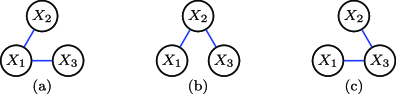
Figure 1: The three trees on $\{X_{1},X_{2},X_{3}\}$.

on $D$ relative to $\mathbf{C}$, thus no term in the sum is positive. Consequently for all $\omega^{*}\in\Omega$, (4.11) does not hold for any tree $\mathfrak{T}$.

Example 2.

In the case $\mathbf{B}=\{X_{1},X_{2}\}=\mathbf{B}_{+}=\mathbf{C}$, there is only one tree on $\mathbf{B}_{+}$, consisting of a single edge $X_{1}\hskip 3.0pt\rule[2.5pt]{12.0pt}{0.3pt}\hskip 3.0ptX_{2}$. Thus if $X_{1}$ and $X_{2}$ have a positive monotonic effect on $D$ (relative to $\mathbf{C}$) then Theorem 4.11 implies that if the following inequality holds for some $\omega\in\Omega$,

$$D_{11}(\omega)-\bigl{(}D_{10}(\omega)+D_{01}(\omega)\bigr{)}+D_{00}(\omega)>0,$$

then $\{X_{1},X_{2}\}$ is irreducible for ${\mathcal{D}}(\mathbf{C},\Omega)$.

Example 3.

If $\mathbf{B}=\{X_{1},X_{2},X_{3}\}=\mathbf{B}_{+}=\mathbf{C}$, then there are three trees on $\mathbf{B}_{+}$; see Figure 1. These correspond to the following conditions:

$$\mathrm{(a)}\quad D_{111}(\omega)-\bigl{(}D_{110}(\omega)+D_{101}(\omega)+D_{011}(\omega)\bigr{)}+\bigl{(}D_{010}(\omega)+D_{001}(\omega)\bigr{)}>0,$$

$$\mathrm{(b)}\quad D_{111}(\omega)-\bigl{(}D_{110}(\omega)+D_{101}(\omega)+D_{011}(\omega)\bigr{)}+\bigl{(}D_{100}(\omega)+D_{001}(\omega)\bigr{)}>0,$$

$$\mathrm{(c)}\quad D_{111}(\omega)-\bigl{(}D_{110}(\omega)+D_{101}(\omega)+D_{011}(\omega)\bigr{)}+\bigl{(}D_{100}(\omega)+D_{010}(\omega)\bigr{)}>0.$$

Thus $\mathbf{B}$ is irreducible for ${\mathcal{D}}(\mathbf{C},\Omega)$ if at least one holds for some $\omega\in\Omega$.

Corollary 4.12.

Let $\mathbf{C}=\mathbf{C}_{1}\,\dot{\cup}\,\mathbf{C}_{2}$, $\mathbf{B}=(\mathbf{B}_{+}\,\dot{\cup}\,\mathbf{B}^{\prime})\in\dot{\mathbb{P}}({\mathbb{L}}(\mathbf{C}_{1}))$, $|\mathbf{B}|=|\mathbf{C}_{1}|$. Suppose that every $L\in\mathbf{B}_{+}$ has a positive monotonic effect on $D$ relative to $\mathbf{C}$, and $\mathbf{W}$ is sufficient to adjust for confounding of $\mathbf{C}$ on $D$. If for some tree ${\mathfrak{T}}$ on $\mathbf{B}_{+}$, and some $\mathbf{c}_{2}$, $\mathbf{w}$ we have

$$0 < E[D|\mathbf{B}=\mathbf{1},\mathbf{C}_{2}=\mathbf{c}_{2},\mathbf{W}=\mathbf{w}]$$

$${}-\sum_{L\in\mathbf{B}}E\bigl{[}D|\mathbf{B}\setminus\{L\}=\mathbf{1},L=0,\mathbf{C}_{2}=\mathbf{c}_{2},\mathbf{W}=\mathbf{w}\bigr{]}$$

$${}+\sum_{\mathbf{E}\in{\mathfrak{T}}}E[D|\mathbf{B}\setminus\mathbf{E}=\mathbf{1},\mathbf{E}=\mathbf{0},\mathbf{C}_{2}=\mathbf{c}_{2},\mathbf{W}=\mathbf{w}],$$

then $\mathbf{B}$ is irreducible for ${\mathcal{D}}(\mathbf{C},\Omega)$.

Directly analogous to the proof of Theorem 4.3.

The special case of the previous Corollary where $|\mathbf{B_{+}}|=|\mathbf{C}|=2$, and $\mathbf{W}=\varnothing$, appears in Rothman and Greenland Rothman1998 ; see also Koopman Koopman1981 . Theorem 4.8 implies that if every literal in $\mathbf{B}$ has a positive monotonic effect on $D$, then we will have $|\mathbf{B}|^{|\mathbf{B}|-2}$ conditions to test, each of which is sufficient to establish the irreducibility of $\mathbf{B}$ for ${\mathcal{D}}(\mathbf{C},\Omega)$. As before, the conditions (4.12) may be tested via $t$-test type statistics or using various statistical models.

As with the results in Section 4.2, we may apply Corollary 3.8 to establish that $\mathbf{B}$ is irreducible for ${\mathcal{D}}(\mathbf{C}\cup\mathbf{C}^{\prime},\Omega)$ if every variable in $\mathbf{C}^{\prime}$ is not causally influenced by variables in $\mathbf{C}$.

4.6 Tests for a minimal sufficient cause under monotonicity

As noted in Section 3.1 if $|\mathbf{B}|=|\mathbf{C}|$, then irreducible conjunctions are also minimal sufficient causes. Thus in this special case, the tests of irreducibility given in Theorem 4.3 and Corollary 4.12 also establish that $\mathbf{B}$ is a minimal sufficient cause relative to $\mathbf{C}$. When $|\mathbf{B}|<|\mathbf{C}|$ these tests do not in general establish this. However, under positive monotonicity assumptions on $\mathbf{C}_{2}$, such tests may be obtained by taking $\mathbf{c}_{2}=\mathbf{0}$:

Proposition 4.13.

Let $\mathbf{C}=\mathbf{C}_{1}\,\dot{\cup}\,\mathbf{C}_{2}$, $\mathbf{B}\in\dot{\mathbb{P}}({\mathbb{L}}(\mathbf{C}_{1}))$, $|\mathbf{B}|=|\mathbf{C}_{1}|$. Suppose every $L\in\mathbf{C}_{2}$ has a positive monotonic effect on $D$ relative to $\mathbf{C}$. If (i) $D_{\mathbf{B}=\mathbf{1},\mathbf{C}_{2}=\mathbf{0}}(\omega^{*})=1$ and (ii) for all $L\in\mathbf{B}$, $D_{\mathbf{B}\setminus\{L\}=\mathbf{1},L=0,\mathbf{C}_{2}=\mathbf{0}}(\omega^{*})=0$, then $\mathbf{B}$ is a minimal sufficient cause for $D$ relative to $\mathbf{C}$ for $\omega^{*}$.

For any $\mathbf{c}_{2}$, $D_{\mathbf{B}=\mathbf{1},\mathbf{C}_{2}=\mathbf{c}_{2}}(\omega^{*})\geq D_{\mathbf{B}=\mathbf{1},\mathbf{C}_{2}=\mathbf{0}}(\omega^{*})=1$ by the monotonicity assumption. Hence $\mathbf{B}$ is a sufficient cause for $D$ relative to $\mathbf{C}$ for $\omega^{*}$. Minimality follows directly from condition (ii).

We have the following corollaries which provide conditions under which $\mathbf{B}$ is a minimal sufficient cause for $D$ relative to $\mathbf{C}$ for some $\omega\in\Omega$, in addition to being irreducible for $\mathcal{D}(\mathbf{C},\Omega)$:

Corollary 4.14.

Let $\mathbf{C}=\mathbf{C}_{1}\,\dot{\cup}\,\mathbf{C}_{2}$, $\mathbf{B}\in\dot{\mathbb{P}}({\mathbb{L}}(\mathbf{C}_{1}))$, $|\mathbf{B}|=|\mathbf{C}_{1}|$. Suppose every $L\in\mathbf{C}_{2}$ has a positive monotonic effect on $D$ relative to $\mathbf{C}$, and $\mathbf{W}$ is sufficient to adjust for confounding of $\mathbf{C}$ on $D$. If (4.3) holds with $\mathbf{c}_{2}=\mathbf{0}$ for some $\mathbf{w}$, then $\mathbf{B}$ is a minimal sufficient cause of $D$ relative to $\mathbf{C}$ for some $\omega\in\Omega$.

The proof follows immediately from Proposition 4.13 and Theorem 4.3.

Corollary 4.15.

Let $\mathbf{C}=\mathbf{C}_{1}\,\dot{\cup}\,\mathbf{C}_{2}$, $\mathbf{B}=(\mathbf{B}_{+}\,\dot{\cup}\,\mathbf{B}^{\prime})\in\dot{\mathbb{P}}({\mathbb{L}}(\mathbf{C}_{1}))$, $|\mathbf{B}|=|\mathbf{C}_{1}|$. Suppose that every $L\in\mathbf{B}_{+}\cup\mathbf{C}_{2}$ has a positive monotonic effect on $D$ relative to $\mathbf{C}$, and $\mathbf{W}$ is sufficient to adjust for confounding of $\mathbf{C}$ on $D$. If (4.12) holds with $\mathbf{c}_{2}=\mathbf{0}$ for some $\mathbf{w}$ and some tree ${\mathfrak{T}}$ on $\mathbf{B}_{+}$, then $\mathbf{B}$ is a minimal sufficient cause of $D$ relative to $\mathbf{C}$ for some $\omega\in\Omega$.

The proof follows immediately from Proposition 4.13 and Corollary 4.12.

5 Singular interactions

In the genetics literature, in the context of two binary genetic factors, $X_{1}$ and $X_{2}$, “compositional” epistasis Bateson1909 , Cordell2002 , Phillips2008 is said to be present if for some $\omega^{\ast}$, $D_{11}(\omega^{\ast})=1$ but $D_{10}(\omega^{\ast})=D_{01}(\omega^{\ast})=D_{00}(\omega^{\ast})=0$; in this case the effect of one genetic factor is effectively masked when the other genetic factor is absent. If $\{X_{1},X_{2}\}$ is a minimal sufficient cause of $D$ relative to $\{X_{1},X_{2}\}$ for $\omega^{*}$ then although this implies $D_{11}(\omega^{\ast})=1$ and $D_{10}(\omega^{\ast})=D_{01}(\omega^{\ast})=0$, it does not imply $D_{00}(\omega^{\ast})=0$. This motivates the following:

Definition 5.1.

A minimal sufficient cause $\mathbf{B}$ for $D$ relative to $\mathbf{C}$ for $\omega^{*}$ is said to be singular if there is no $\mathbf{B}^{\prime}\in\dot{\mathbb{P}}(\mathbb{L}(\mathbf{C}))$, $\mathbf{B}^{\prime}\neq\mathbf{B}$, forming a minimal sufficient cause for $D$ relative to $\mathbf{C}$ for $\omega^{*}$. $\mathbf{B}$ is singular for $\mathcal{D}(\mathbf{C},\Omega)$ if $\mathbf{B}$ is singular relative to $\mathbf{C}$ for some $\omega^{*}\in\Omega$.

If $\mathbf{B}$ is singular for ${\mathcal{D}}(\mathbf{C},\Omega)$, then we will also refer to a singular interaction between the components of $\mathbf{B}$. We now characterize singularity in terms of potential outcomes:

Theorem 5.2

Let $\mathbf{C}=\mathbf{C}_{1}\cup\mathbf{C}_{2}$, $\mathbf{B}\in\dot{\mathbb{P}}(\mathbb{L}(\mathbf{C}_{1}))$, $|\mathbf{B}|=|\mathbf{C}_{1}|$. Then $\mathbf{B}$ is singular for $\mathcal{D}(\mathbf{C},{\Omega})$ if and only if there exists $\omega^{\ast}\in{\Omega}$ such that

$$\mbox{for all values }\mathbf{c}_{2}^{\ast},\mathbf{b}\dvtx\qquad D_{\mathbf{B}=\mathbf{b},\mathbf{C}_{2}=\mathbf{c}_{2}^{\ast}}\bigl{(}\omega^{\ast}\bigr{)}=1\quad\Longleftrightarrow\quad\mathbf{b}=\mathbf{1}.$$ (12)

Note that (12) is equivalent to

$$D_{\mathbf{C}=\mathbf{c}}\bigl{(}\omega^{\ast}\bigr{)}=\Bigl{(}\bigwedge(\mathbf{B})\Bigr{)}_{\mathbf{c}}\qquad\mbox{for all }\mathbf{c}.$$ (13)

Thus if $\mathbf{B}$ is singular for $\mathcal{D}(\mathbf{C},\Omega)$, then there is some individual $\omega^{*}$ whose potential outcomes are given by the single conjunction $\mathbf{B}$.

By definition, $\mathbf{B}$ is a sufficient cause for $D$ for $\omega^{*}$ if and only if ($\mathbf{b}=\mathbf{1}$ $\Rightarrow$ $D_{\mathbf{B}=\mathbf{b},\mathbf{C}_{2}=\mathbf{c}_{2}^{*}}(\omega^{*})=1$). Thus it is sufficient to show that, assuming $\mathbf{B}$ is a minimal sufficient cause for $D$ for $\omega^{*}$, there are no other minimal sufficient causes of $D$ for $\omega^{*}$ if and only if ($D_{\mathbf{B}=\mathbf{b},\mathbf{C}_{2}=\mathbf{c}_{2}^{*}}(\omega^{*})=1$ $\Rightarrow$ $\mathbf{b}=\mathbf{1}$).

Suppose $\mathbf{B}$ is the only minimal sufficient cause for $D$ for $\omega^{*}$, but that for some $\mathbf{b}^{*}\neq\mathbf{1}$, $D_{\mathbf{B}=\mathbf{b}^{*},\mathbf{C}_{2}=\mathbf{c}_{2}^{*}}(\omega^{*})=1$. Let $\mathbf{B}^{\dagger}\equiv\mathbf{B}^{[\mathbf{B}=\mathbf{b}^{*},\mathbf{C}_{2}=\mathbf{c}_{2}^{*}]}$. $\mathbf{B}^{\dagger}$ forms a sufficient cause for $D$ for $\omega^{*}$, and $\mathbf{B}\nsubseteq\mathbf{B}^{\dagger}$. Hence there is some $\mathbf{B}^{\prime}\subseteq\mathbf{B}^{\dagger}$ that is a minimal sufficient cause for $D$ for $\omega^{*}$, and $\mathbf{B}\neq\mathbf{B}^{\dagger}$, a contradiction.

Conversely suppose ($D_{\mathbf{B}=\mathbf{b},\mathbf{C}_{2}=\mathbf{c}_{2}^{*}}(\omega^{*})=1$ $\Rightarrow$ $\mathbf{b}=\mathbf{1}$) but there exists another minimal sufficient cause $\mathbf{B}^{\prime}$ for $D$ for $\omega^{*}$, and $\mathbf{B}\neq\mathbf{B}^{\dagger}$. Since $\mathbf{B}^{\prime}$ is minimal, $\mathbf{B}\nsubseteq\mathbf{B}^{\prime}$. Thus there exists a $\tilde{\mathbf{c}}$ such that $(\mathbf{B})_{\tilde{\mathbf{c}}}\neq\mathbf{1}$, but $(\mathbf{B}^{\prime})_{\tilde{\mathbf{c}}}=\mathbf{1}$ and hence $D_{\mathbf{C}={\tilde{\mathbf{c}}}}(\omega^{*})=1$, a contradiction.

Corollary 5.3.

For $\mathcal{D}(\mathbf{C},{\Omega})$, if $\mathbf{B}$ is singular then $\mathbf{B}$ is irreducible.

The proof follows immediately from (12) and the definition of irreducibility.

Theorem 5.4 relates singular interactions to properties of the set of sufficient cause representations for $\mathcal{D}(\mathbf{C},{\Omega})$.

Theorem 5.4

Let $\mathbf{B}\in\dot{\mathbb{P}}(\mathbb{L}(\mathbf{C}))$. $\mathbf{B}$ is singular for $\mathcal{D}(\mathbf{C},{\Omega})$ if and only if there exists $\omega^{\ast}\in{\Omega}$ such that in every representation $(\mathbf{A},\mathfrak{B})$ for $\mathcal{D}(\mathbf{C},{\Omega})$, (i) for all $\mathbf{B}^{\ast}\in\dot{\mathbb{P}}(\mathbb{L}(\mathbf{C}))$, with $|\mathbf{B}^{\ast}|=|\mathbf{C}|$ and $\mathbf{B}\subseteq\mathbf{B}^{\ast}$ there exists $\mathbf{B}_{i}\in\mathfrak{B}$ with $\mathbf{B}_{i}\subseteq\mathbf{B}^{\ast}$ and $A_{i}(\omega^{\ast})=1$; (ii) for all $\mathbf{B}_{i}\in\mathfrak{B}$ such that $\mathbf{B}\nsubseteq\mathbf{B}_{i}$, $A_{i}(\omega^{\ast})=0$.

Let $\mathbf{C}=\mathbf{C}_{1}\,\dot{\cup}\,\mathbf{C}_{2}$, where $\mathbf{B}\in\dot{\mathbb{P}}(\mathbb{L}(\mathbf{C}_{1}))$, and $|\mathbf{B}|=|\mathbf{C}_{1}|$.

$(\Rightarrow)$ Suppose $\mathbf{B}$ is singular for $\mathcal{D}(\mathbf{C},{\Omega})$, so that some $\omega^{\ast}\in{\Omega}$ satisfies (13). Then for any representation $(\mathbf{A},\mathfrak{B})$ for $\mathcal{D}(\mathbf{C},{\Omega})$ and any $\mathbf{B}^{\ast}$ such that $|\mathbf{B}^{\ast}|=|\mathbf{C}|$ and $\mathbf{B}\subseteq\mathbf{B}^{\ast}$, we can select values $\mathbf{c}_{2}^{\ast}$ so that $\mathbf{B}^{\ast}=\mathbf{B}^{[\mathbf{B}=\mathbf{1},\mathbf{C}_{2}=\mathbf{c}_{2}^{\ast}]}$. Since $D_{\mathbf{B}=\mathbf{1},\mathbf{C}_{2}=\mathbf{c}_{2}^{\ast}}(\omega^{\ast})=1$ there exists $A_{i}\in\mathbf{A}$, $\mathbf{B}_{i}\in\mathfrak{B}$ with $A_{i}(\omega^{\ast})=1$ and $(\bigwedge(\mathbf{B}_{i}))_{\mathbf{B}=\mathbf{1},\mathbf{C}_{2}=\mathbf{c}_{2}^{\ast}}=1$. Thus $\mathbf{B}_{i}\subseteq\mathbf{B}^{\ast}$, so (i) holds. For all $\mathbf{B}_{i}\in\mathfrak{B}$ such that $\mathbf{B}\nsubseteq\mathbf{B}_{i}$, we can choose $\widetilde{\mathbf{B}}\in\dot{\mathbb{P}}(\mathbb{L}(\mathbf{C}_{1}))$, $|\widetilde{\mathbf{B}}|=|\mathbf{C}_{1}|$ with $\widetilde{\mathbf{B}}\neq\mathbf{B}$ and values $\tilde{\mathbf{c}}_{2}$ so that $\mathbf{B}_{i}\subseteq\mathbf{B}^{[\widetilde{\mathbf{B}}=\mathbf{1},\mathbf{C}_{2}=\tilde{\mathbf{c}}_{2}]}$. Since $D_{\widetilde{\mathbf{B}}=\mathbf{1},\mathbf{C}_{2}=\tilde{\mathbf{c}}_{2}}(\omega^{\ast})=0$ we have $A_{i}(\omega^{\ast})=0$ since $(\bigwedge(\mathbf{B}_{i}))_{\widetilde{\mathbf{B}}=\mathbf{1},\mathbf{C}_{2}=\tilde{\mathbf{c}}_{2}}=1$, so (ii) holds as required.

$(\Leftarrow)$ Suppose there exists $\omega^{\ast}\in{\Omega}$ such that every representation $(\mathbf{A},\mathfrak{B})$ satisfies (i) and (ii). We will show that (12) holds. For any values $\mathbf{c}_{2}^{\ast}$ let $\mathbf{B}^{\ast}\equiv\mathbf{B}^{[\mathbf{B}=\mathbf{1},\mathbf{C}_{2}=\mathbf{c}_{2}^{\ast}]}$, so $|\mathbf{B}^{\ast}|=|\mathbf{C}|$ and $\mathbf{B}\subseteq\mathbf{B}^{\ast}$. Thus by (i) there exists $\mathbf{B}_{i}\in\mathfrak{B}$ with $\mathbf{B}_{i}\subseteq\mathbf{B}^{\ast}$ and $A_{i}(\omega^{\ast})=1$. Hence $D_{\mathbf{B}=\mathbf{1},\mathbf{C}_{2}=\mathbf{c}_{2}^{\ast}}(\omega^{\ast})=1$ since $A_{i}(\omega^{\ast})=1$ and $(\bigwedge(\mathbf{B}_{i}))_{\mathbf{B}=\mathbf{1},\mathbf{C}_{2}=\mathbf{c}_{2}^{\ast}}=1$. Conversely for any $\mathbf{b}^{\prime}\neq\mathbf{1}$, let $\mathbf{B}^{\prime}\equiv\mathbf{B}^{[\mathbf{B}=\mathbf{b}^{\prime}]}$, so $|\mathbf{B}^{\prime}|=|\mathbf{C}_{1}|$ with $\mathbf{B}^{\prime}\neq\mathbf{B}$. Thus for all $\mathbf{B}_{i}\in\mathfrak{B}$ such that $(\bigwedge(\mathbf{B}_{i}))_{\mathbf{B}^{\prime}=\mathbf{1},\mathbf{C}_{2}=\mathbf{c}_{2}^{\ast}}=1$, $\mathbf{B}\nsubseteq\mathbf{B}_{i}$ and thus by (ii) $A_{i}(\omega^{\ast})=0$. Hence $D_{\mathbf{B}^{\prime}=\mathbf{1},\mathbf{C}_{2}=\mathbf{c}_{2}^{\ast}}(\omega^{\ast})=0$.

We now consider results relevant for testing for singular interactions with or without monotonicity assumptions.

Theorem 5.5

Let $\mathbf{B}=\mathbf{B}_{+}\,\dot{\cup}\,\mathbf{B}^{\prime}\in\dot{\mathbb{P}}(\mathbb{L}(\mathbf{C}))$, $|\mathbf{B}|=|\mathbf{C}|$ and suppose that every $L\in\mathbf{B}_{+}$ has a positive monotonic effect on $D$ relative to $\mathbf{C}$. If for some tree $\mathfrak{T}$ on $\mathbf{B}_{+}$ and some $\omega^{\ast}\in{\Omega}$, we have

$$D_{\mathbf{B}=\mathbf{1}}\bigl{(}\omega^{\ast}\bigr{)}-\sum_{L\in\mathbf{B}_{+}}D_{\mathbf{B}\setminus\{L\}=\mathbf{1},L=0}\bigl{(}\omega^{\ast}\bigr{)}$$

(14)

$$\qquad{}-\sum_{\widetilde{\mathbf{B}}\dvtx\varnothing\neq\widetilde{\mathbf{B}}\subseteq\mathbf{B}^{\prime}}D_{\mathbf{B}\setminus\widetilde{\mathbf{B}}=\mathbf{1},\widetilde{\mathbf{B}}=\mathbf{0}}\bigl{(}\omega^{\ast}\bigr{)}+\sum_{\mathbf{E}\in\mathfrak{T}}D_{\mathbf{B}\setminus\mathbf{E}=\mathbf{1},\mathbf{E}=\mathbf{0}}\bigl{(}\omega^{\ast}\bigr{)}>0,$$

then $\mathbf{B}$ is singular for $\mathcal{D}(\mathbf{C},{\Omega})$.

By Theorem 5.4, $\mathbf{B}$ is singular for $\mathcal{D}(\mathbf{C},{\Omega})$ if and only if

$$\mbox{for some }\omega^{\ast}\in{\Omega},\qquad D_{\mathbf{B}=\mathbf{1}}\bigl{(}\omega^{\ast}\bigr{)}-\sum_{\widetilde{\mathbf{B}}\subseteq\mathbf{B}}D_{\mathbf{B}\setminus\widetilde{\mathbf{B}}=\mathbf{1},\widetilde{\mathbf{B}}=\mathbf{0}}\bigl{(}\omega^{\ast}\bigr{)}>0.$$ (15)

Suppose for a contradiction that (15) does not hold but (5.5) holds for some $\omega^{*}\in\Omega$. Since $\mathbf{B}_{+}$ has a positive monotonic effect on $D$ relative to $\mathbf{C}$, if $\widetilde{\mathbf{B}}\subseteq\mathbf{B}$ is such that $\widetilde{\mathbf{B}}\cap\mathbf{B}_{+}\neq\varnothing$, then $D_{\mathbf{B}\setminus\widetilde{\mathbf{B}}=\mathbf{1},\widetilde{\mathbf{B}}=\mathbf{0}}(\omega^{*})=1$ implies $D_{\mathbf{B}\setminus\{L\}=\mathbf{1},L=0}(\omega^{*})=1$ for some $L\in\widetilde{\mathbf{B}}$. Hence for all $\omega\in\Omega$,

$$\qquad D_{\mathbf{B}=\mathbf{1}}(\omega)-\sum_{L\in\mathbf{B}}D_{\mathbf{B}\setminus\{L\}=\mathbf{1},L=0}(\omega)-\sum_{\widetilde{\mathbf{B}}\subseteq\mathbf{B}^{\prime},|\widetilde{\mathbf{B}}|\geq 2}D_{\mathbf{B}\setminus\widetilde{\mathbf{B}}=\mathbf{1},\widetilde{\mathbf{B}}=\mathbf{0}}(\omega)\leq 0.$$ (16)

By applying the same argument to the first two terms on the left-hand side of (16) as was applied in the proof of Theorem 4.11, we have that (5.5) does not hold for all $\omega\in\Omega$, which is a contradiction.

The following corollary to Theorem 5.5 generalizes the discussion in VanderWeele2010a , VanderWeele2010b to an arbitrary number of dichotomous factors:

Corollary 5.6.

Let $\mathbf{B}=\mathbf{B}_{+}\,\dot{\cup}\,\mathbf{B}^{\prime}\in\dot{\mathbb{P}}(\mathbb{L}(\mathbf{C}))$, $|\mathbf{B}|=|\mathbf{C}|$. Suppose that every $L\in\mathbf{B}_{+}$ has a positive monotonic effect on $D$ relative to $\mathbf{B}$, and $\mathbf{W}$ is sufficient to adjust for confounding of $\mathbf{C}$ on $D$. If for some tree $\mathfrak{T}$ on $\mathbf{B}_{+}$, and some $\mathbf{w}$, we have

$$0 < E[D|\mathbf{B}=\mathbf{1},\mathbf{W}=\mathbf{w}]-\sum_{L\in\mathbf{B}_{+}}E\bigl{[}D|\mathbf{B}\setminus\{L\}=\mathbf{1},L=0,\mathbf{W}=\mathbf{w}\bigr{]}$$

$${}-\sum_{\widetilde{\mathbf{B}}\dvtx\varnothing\neq\widetilde{\mathbf{B}}\subseteq\mathbf{B}^{\prime}}E[D|\mathbf{B}\setminus\widetilde{\mathbf{B}}=\mathbf{1},\widetilde{\mathbf{B}}=\mathbf{0},\mathbf{W}=\mathbf{w}]$$

$${}+\sum_{\mathbf{E}\in\mathfrak{T}}E[D|\mathbf{B}\setminus\mathbf{E}=\mathbf{1},\mathbf{E}=\mathbf{0},\mathbf{W}=\mathbf{w}],$$

then $\mathbf{B}$ is singular for $\mathcal{D}(\mathbf{C},{\Omega})$.

By applying Proposition 4.2 to each term in (5.5), the proof is complete.

Condition (5.6) leads directly to a statistical test of compositional epistasis. This is notable since some claims in the genetics literature appear to suggest that such tests did not exist Cordell2002 .

As stated in the next corollary, from Theorem 5.5, if all or all but one of the elements of $\mathbf{B}$ have positive monotonic effects on $D$, then singularity and irreducibility coincide:

Corollary 5.7.

Suppose $|\mathbf{B}|=|\mathbf{C}|$ and that for all or all but one of $B_{i}\in\mathbf{B}$, $B_{i}$ has a positive monotonic effect on $D$ relative to $\mathbf{B}$, then $\mathbf{B}$ is singular for $\mathcal{D}(\mathbf{C},{\Omega})$ if and only if $\mathbf{B}$ is irreducible for $\mathcal{D}(\mathbf{C},{\Omega})$.

An important consequence of this corollary is that when there is at most one variable that does not have a positive monotonic effect, condition (4.12) establishes that $\mathbf{B}$ is singular in addition to being irreducible for $\mathcal{D}(\mathbf{C},{\Omega})$.

Let $\mathbf{B}^{\prime}$ denote the one or zero elements of $\mathbf{B}$ that do not have a monotonic effect on $D$ relative to $\mathbf{C}$. If $\mathbf{B}$ is irreducible for $\mathcal{D}(\mathbf{C},{\Omega})$, then by the argument in the proof of Theorem 4.11,

$$D_{\mathbf{B}=\mathbf{1}}\bigl{(}\omega^{\ast}\bigr{)}-\sum_{L\in\mathbf{B}}D_{\mathbf{B}\setminus\{L\}=\mathbf{1},L=0}\bigl{(}\omega^{\ast}\bigr{)}+\sum_{\mathbf{E}\in\mathfrak{T}}D_{\mathbf{B}\setminus\mathbf{E}=\mathbf{1},\mathbf{E}=\mathbf{0}}\bigl{(}\omega^{\ast}\bigr{)}>0.$$

Since the third term on the left-hand side of (5.5) vanishes when $|\mathbf{B}^{\prime}|\leq 1$, it follows that $\mathbf{B}$ is singular for $\mathcal{D}(\mathbf{C},{\Omega})$. The converse is given in Corollary 5.3.

Corollary 5.8.

Suppose $|\mathbf{B}|=|\mathbf{C}|$ and that for all or all but one of $B_{i}\in\mathbf{B}\,\dot{\cup}\,\mathbf{C}^{\prime}$, $B_{i}$ has a positive monotonic effect on $D$ relative to $\mathbf{B}\cup\mathbf{C}^{\prime}$, for all $X^{\prime}\in\mathbf{C}^{\prime}$, $X^{\prime}$ is not causally influenced by $\mathbf{C}$ and $\mathbf{B}$ is singular for $\mathcal{D}(\mathbf{C},{\Omega})$, then $\mathbf{B}$ is singular for $\mathcal{D}(\mathbf{C}\cup\mathbf{C}^{\prime},{\Omega})$.

By Corollary 5.7, $\mathbf{B}$ is irreducible relative to $\mathcal{D}(\mathbf{C},{\Omega})$. Hence by Corollary 3.8 $\mathbf{B}$ is irreducible relative to $\mathcal{D}(\mathbf{C}\cup\mathbf{C}^{\prime},{\Omega})$. The conclusion then follows from a further application of Corollary 5.7.

5.1 Relation to Pearl’s probability of causation

Pearl Pearl2000 , Chapter 9, defined the probability of necessity and sufficiency (PNS) of cause $X$ for outcome $D$ to be $P(D_{X=1}(\omega)=1,D_{X=0}(\omega)=0)$. In other words $\operatorname{PNS}(D,X)$ is the probability that $D$ would occur if $X$ occurred and would not have done so had $X$ not occurred. We generalize this to the setting in which there are multiple causes $\mathbf{B}$:

Definition 5.9.

For $\mathbf{B}\subseteq\dot{\mathbb{P}}({\mathbb{L}}(\mathbf{C}))$, the probability of necessity and sufficiency of $\mathbf{B}$ causing $D$ is

$$\operatorname{PNS}(D,\mathbf{B})\equiv P(D_{\mathbf{B}=\mathbf{1}}=1\mbox{ and for all }\mathbf{b}\neq\mathbf{1},D_{\mathbf{B}=\mathbf{b}}=0).$$

Thus $\operatorname{PNS}(D,\mathbf{B})$ is the probability that $D$ would occur if every literal $L\in\mathbf{B}$ occurred and would not have done so had at least one literal in $\mathbf{B}$ not occurred.

Proposition 5.10.

If $|\mathbf{B}|=|\mathbf{C}|$, then $\operatorname{PNS}(D,\mathbf{B})>0$ if and only if $\mathbf{B}$ is singular for $\mathcal{D}(\mathbf{C},{\Omega})$.

The proof follows directly from Theorem 5.4 and Definition 5.9.

This connection also provides an interpretation for condition (5.6). For expositional convenience in the following proposition, we assume that $\mathbf{B}$ and $D$ are unconfounded and do not make monotonicity assumptions; it would be straightforward to do so.

Proposition 5.11.

Under the conditions of Corollary 5.6, with $\mathbf{W}=\varnothing=\mathbf{B}_{+}$, $\operatorname{PNS}(\mathbf{B},D)$ is bounded below by the right-hand side of (5.6).

$$\operatorname{PNS}(D,\mathbf{B}) = P(D_{\mathbf{B}=\mathbf{1}}=1\mbox{ and for all }\mathbf{b}\neq\mathbf{1},D_{\mathbf{B}=\mathbf{b}}=0)$$

$$\geq P(D_{\mathbf{B}=\mathbf{1}}=1)+P(\mbox{for all }\mathbf{b}\neq\mathbf{1},D_{\mathbf{B}=\mathbf{b}}=0)-1$$

$$= P(D_{\mathbf{B}=\mathbf{1}}=1)-P(\mbox{for some }\mathbf{b}\neq\mathbf{1},D_{\mathbf{B}=\mathbf{b}}=1)$$

$$\geq P(D_{\mathbf{B}=\mathbf{1}}=1)-\sum_{\mathbf{b}\neq\mathbf{1}}P(D_{\mathbf{B}=\mathbf{b}}=1)$$

$$= E[D=1|{\mathbf{B}=\mathbf{1}}]-\sum_{\mathbf{b}\neq\mathbf{1}}E[D|{\mathbf{B}=\mathbf{b}}]$$

which is the right-hand side of (5.6) with $\mathbf{W}=\varnothing=\mathbf{B}_{+}$.

This generalizes some of the lower bounds on $\operatorname{PNS}(D,X)$ given by Pearl Pearl2000 , Section 9.2.

6 Relation to statistical models with linear links

In related work VanderWeele2008a it is noted that the presence of interaction terms in statistical models do not, in general, correspond to sufficient conditions for irreducibility. Consider, for example, a saturated Bernoulli regression model for $D$ with identity link and binary regressors $\mathbf{C}=\{X_{1},\ldots,X_{p}\}$,

$$E[D|\mathbf{C}=\mathbf{c}]=\sum_{\widetilde{\mathbf{B}}\subseteq\mathbf{C}}\beta_{\widetilde{\mathbf{B}}}\Bigl{(}\bigwedge(\widetilde{\mathbf{B}})\Bigr{)}_{\mathbf{c}}.$$ (18)

Note that with $\mathbf{c}=(x_{1},\ldots,x_{p})$, then $(\bigwedge(\widetilde{\mathbf{B}}))_{\mathbf{c}}=\prod_{X_{i}\in\widetilde{\mathbf{B}}}x_{i}$, the usual product interaction term. The conditions, given earlier, for detecting the presence of irreducibility and singularity lead to linear restrictions on the regression coefficients $\beta_{\widetilde{\mathbf{B}}}$.

$$\sum_{\widetilde{\mathbf{B}}\subseteq\mathbf{C}}m_{\widetilde{\mathbf{B}}}\beta_{\widetilde{\mathbf{B}}}>0.$$ (19)

Note that (19) includes an intercept $\beta_{\varnothing}$. First we define

$$\deg_{\mathfrak{T}}(L)\equiv\bigl{|}\{\mathbf{E}|\mathbf{E}\in{\mathfrak{T}},L\in\mathbf{E}\}\bigr{|},$$

the degree of $L$ in a tree $\mathfrak{T}$, to be the number of edges in $\mathfrak{T}$ that contain $L$.

Proposition 6.1.

Under the conditions of Theorem 4.11, with $\mathbf{B}=\mathbf{C}$, condition (4.11) is equivalent to restriction (19) with $m_{\widetilde{\mathbf{B}}}=m_{\widetilde{\mathbf{B}}}^{\mathrm{irred}}$ where

$$m_{\widetilde{\mathbf{B}}}^{\mathrm{irred}} \equiv 1-|\mathbf{B}\setminus\widetilde{\mathbf{B}}|+|\mathfrak{T}|$$

$${}-\sum_{L\in\widetilde{\mathbf{B}}\cap\mathbf{B}_{+}}\deg_{\mathfrak{T}}(L)+\bigl{|}\{\mathbf{E}|\mathbf{E}\in{\mathfrak{T}},\mathbf{E}\subseteq\widetilde{\mathbf{B}}\cap\mathbf{B}_{+}\}\bigr{|}.$$

Note that since $\mathfrak{T}$ is a tree on $\mathbf{B}_{+}$, the last term in (6.1) has a natural graphical interpretation as the number of edges in the “induced subgraph” of $\mathfrak{T}$ on the subset $\widetilde{\mathbf{B}}$. Definition (6.1) also subsumes condition (4.3) given in Theorem 4.3 (without monotonicity), in which case the last three terms in (6.1) vanish. Though Proposition 6.1 assumes that $\mathbf{C}_{2}=\varnothing$, the condition given by (19) and (6.1) continues to apply in the case where $\mathbf{c}_{2}=\mathbf{0}$, as in Corollaries 4.14 and 4.15; obvious extensions apply to the case where $\mathbf{c}_{2}\neq\mathbf{0}$.

This follows by counting the number (and sign) of expectations in (4.11) for which $\widetilde{\mathbf{B}}$ is a subset of the variables assigned the value $1$ in the conditioning event. The first two terms in (4.11) correspond, respectively, to the first two terms in (6.1). The remaining three terms in (6.1) correspond to the last sum in (4.11): $|\mathfrak{T}|$, the number of edges in $\mathfrak{T}$, is the total number of terms in the sum. The sum over degrees subtracts the number of terms in which some $L\in\widetilde{\mathbf{B}}$ is assigned zero. Since this double counts terms corresponding to edges contained in $\widetilde{\mathbf{B}}$, the last term corrects for this.

Proposition 6.2.

Under the conditions of Theorem 5.5, with $\mathbf{B}=\mathbf{C}$, condition (5.5) is equivalent to restriction (19) with $m_{\widetilde{\mathbf{B}}}=m_{\widetilde{\mathbf{B}}}^{\mathrm{sing}}$ where

$$m_{\widetilde{\mathbf{B}}}^{\mathrm{sing}}\equiv m_{\widetilde{\mathbf{B}}}^{\mathrm{irred}}+\bigl{(}\bigl{|}\mathbf{B}^{\prime}\setminus\widetilde{\mathbf{B}}\bigr{|}\bigr{)}-\bigl{(}2^{|\mathbf{B}^{\prime}\setminus\widetilde{\mathbf{B}}|}-1\bigr{)}.$$ (21)

Expression (21) follows from another counting argument similar to the proof of Proposition 6.1, together with the observation that conditions (4.11) and (5.5) only differ in that the terms in the sum over $L$ in (4.11) for $L\in\mathbf{B}^{\prime}$ are replaced by a sum over all subsets of $\mathbf{B}^{\prime}$.

Example 4 ((Two-way interactions)).

Consider the saturated Bernoulli regression with identity link with $\mathbf{C}=\{X_{1},X_{2}\}$.

$$E[D|X_{1}=x_{1},X_{2}=x_{2}]=\beta_{\varnothing}+\beta_{1}x_{1}+\beta_{2}x_{2}+\beta_{12}x_{1}x_{2}.$$

Suppose that $X_{1}$ and $X_{2}$ are unconfounded with respect to $D$, so (8) holds with $\mathbf{W}=\varnothing$. Proposition 6.1 implies that $\{X_{1},X_{2}\}$ is irreducible relative to $\mathbf{C}$ if $\beta_{12}>\beta_{\varnothing}$; Proposition 6.2 implies that $\{X_{1},X_{2}\}$ is singular relative to $\mathbf{C}$ if $\beta_{12}>2\beta_{\varnothing}$. If one of $X_{1}$ or $X_{2}$ have positive monotonic effects on $D$ relative to $\mathbf{C}$, then Proposition 6.1 and Corollary 5.7 imply that $\{X_{1},X_{2}\}$ is both irreducible and singular relative to $\mathbf{C}$ if $\beta_{12}>\beta_{\varnothing}$. If $X_{1}$ and $X_{2}$ have positive monotonic effects on $D$ relative to $\mathbf{C}$, then Proposition 6.1 and Corollary 5.7 imply that $\{X_{1},X_{2}\}$ is both irreducible and singular relative to $\mathbf{C}$ if $\beta_{12}>0$.

Thus only under the assumption of positive monotonic effects for both $X_{1}$ and $X_{2}$ does the sufficient condition for the irreducibility and singularity of $\{X_{1},X_{2}\}$ coincide with the classical two-way interaction term $\beta_{12}$ being positive. Note that under the assumption of negative monotonic effects of $X_{1}$ and $X_{2}$ on $D$, $\beta_{12}<0$ is equivalent to irreducibility and singularity for $\bar{D}\equiv(1-D)$; see vanderweeleremarks2011 for this and other remarks on recoding of exposures or outcomes.

It also follows from Proposition 3.4 that if $\{X_{1},X_{2}\}$ is irreducible relative to $\mathbf{C}$, then there exists some $\omega\in\Omega$ for whom $\{X_{1},X_{2}\}$ is a minimal sufficient cause relative to $\mathbf{C}$ (since $|\mathbf{B}|=|\mathbf{C}|$).

Example 5 ((Three-way interactions)).

The saturated Bernoulli regression with three binary variables and a identity link can be written as

$$E[D=1|X_{1}=x_{1},X_{2}=x_{2},X_{3}=x_{3}]$$

$$\qquad=\beta_{\varnothing}+\beta_{1}x_{1}+\beta_{2}x_{2}+\beta_{3}x_{3}+\beta_{12}x_{1}x_{2}+\beta_{13}x_{1}x_{3}$$

$$\qquad\quad{}+\beta_{23}x_{2}x_{3}+\beta_{123}x_{1}x_{2}x_{2}.$$

Suppose that $\mathbf{C}=\{X_{1},X_{2},X_{3}\}$ is unconfounded for $D$. Proposition 6.1 implies that $\{X_{1},X_{2},X_{3}\}$ is irreducible relative to $\mathbf{C}$ if

$$\beta_{123}>2\beta_{\varnothing}+\beta_{1}+\beta_{2}+\beta_{3}.$$ (22)

It follows from Proposition 3.4 that if $\{X_{1},X_{2},X_{3}\}$ is irreducible relative to $\mathbf{C}$, then there exists some $\omega\in\Omega$ for whom $\{X_{1},X_{2},X_{3}\}$ is a minimal sufficient cause relative to $\mathbf{C}$ (since $|\mathbf{B}|=|\mathbf{C}|$).

Proposition 6.2 implies $\{X_{1},X_{2},X_{3}\}$ is singular relative to $\mathbf{C}$ if

$$\beta_{123}>6\beta_{\varnothing}+2\beta_{1}+2\beta_{2}+2\beta_{3}.$$

However, if $X_{1}$, $X_{2}$ and $X_{3}$ have positive monotonic effects on $D$ (relative to $\mathbf{C}$), then Proposition 6.1 implies $\{X_{1},X_{2},X_{3}\}$ is irreducible relative to $\mathbf{C}$ if any of the following hold:

$$\beta_{123}>\beta_{1},\qquad\beta_{123}>\beta_{2},\qquad\beta_{123}>\beta_{3};$$ (23)

equivalently, $\beta_{123}>\min\{\beta_{1},\beta_{2},\beta_{3}\}$. By Corollary 5.7 this also establishes that $\{X_{1},X_{2},X_{3}\}$ is singular relative to $\mathbf{C}$.

If only $X_{1}$ and $X_{2}$ have positive monotonic effects on $D$ relative to $\mathbf{C}$, then Proposition 6.1 implies that $\{X_{1},X_{2},X_{3}\}$ is irreducible relative to $\mathbf{C}$ if

$$\beta_{123}>\beta_{\varnothing}+\beta_{1}+\beta_{2}.$$ (24)

By Corollary 5.7, condition (24) also implies that $\{X_{1},X_{2},X_{3}\}$ is singular relative to $\mathbf{C}$ (since only $X_{3}$ does not have a positive monotonic effect on $D$). As we would expect condition (24) is weaker than (22), but stronger than any of the conditions in (23). If only one potential cause has a monotonic effect on $D$ relative to $\mathbf{C}$, then we can only use (22) to establish irreducibility.

Thus for three-way interactions, $\beta_{123}>0$ does not correspond to any of the sufficient conditions for irreducibility or singularity of $\{X_{1},X_{2},X_{3}\}$ relative to $\mathbf{C}$, regardless of whether or not monotonicity assumptions hold.

7 Interpretation of sufficient cause models

As mentioned in Section 2.1 the observed data for an individual $(\mathbf{C}(\omega),D(\omega))$ represents a strict subset of the potential outcomes ${\mathcal{D}}(\mathbf{C},\omega)$; this is the “fundamental problem of causal inference.” Further, as we have seen, for a given set of potential outcomes there can exist different determinative sets of minimal sufficient causes ${\mathfrak{B}}$ for the same set of potential outcomes; see (3) and (4). Thus we have the following for an individual:

$$\begin{array}[]{ccccc}\vdots&\searrow&\vdots&\searrow&\\[3.0pt] {\mathfrak{B}}&\rightarrow&{\mathcal{D}}(\mathbf{C},\omega)&\rightarrow&\bigl{(}\mathbf{C}(\omega),D(\omega)\bigr{)}.\\ \vdots&\nearrow&\vdots&\nearrow&\\ &\mbox{\scriptsize many-one}&&\mbox{\scriptsize many-one}&\end{array}$$ (25)

It is typically impossible to know the set of potential outcomes for an individual ${\mathcal{D}}(\mathbf{C},\omega)$, even when $\mathbf{C}=\{X\}$, even from randomized experiments. However, possession of this knowledge would permit one to predict how a given individual would respond under any given pattern of exposures $\mathbf{C}=\mathbf{c}$.

The results in this paper demonstrate that, given data from a randomized experiment (or when sufficient variables are measured to adjust for confounding), it is possible to infer the existence of an individual for whom all sets of minimal sufficient causes $\mathfrak{B}$ have certain features in common. However, given the double many-one relationship (25), and the fact that the set of potential outcomes ${\mathcal{D}}(\mathbf{C},\omega)$, if they were known, apparently address all potential counterfactual queries, it is natural to ask what is to be gained by considering such representations. We now motivate our results by presenting several different interpretations of sufficient cause representations.

7.1 The descriptive interpretation

Under this view, sets of minimal sufficient causes are merely a way to describe the set of potential outcomes ${\mathcal{D}}(\mathbf{C},\Omega)$. The representation $(\mathbf{A},{\mathfrak{B}})$ may be more compact; compare Table 2 and (1). Extending this to a population $\Omega$, the variables $\mathbf{A}$ in a representation $(\mathbf{A},{\mathfrak{B}})$ merely describe subpopulations with particular patterns of potential outcomes.

Knowing that there exists an individual for whom all representations ${\mathfrak{B}}$ have certain features in common provides qualitative information about the set of potential outcomes.

For two binary causes $\{X_{1},X_{2}\}$, Theorem 3.2 implies that $\{X_{1},X_{2}\}$ is irreducible relative to $\mathbf{C}$ for $\omega^{\ast}$ if $D_{11}(\omega^{\ast})=1$ and $D_{10}(\omega^{\ast})=D_{01}(\omega^{\ast})=0$. Such a pattern is of interest insofar as it indicates that the causal process resulting in this individual’s potential outcomes ${\mathcal{D}}(\mathbf{C},\omega^{\ast})$ is such that (for some setting of the variables in $\mathbf{C}\setminus\{X_{1},X_{2}\}$), $D=1$ if both $X_{1}=1$ and $X_{2}=1$, but not when $X_{1}=1$ and $X_{2}=0$ or vice versa.

Similarly it follows from Theorem 5.2 that if $\{X_{1},X_{2}\}$ is singular relative to $\mathbf{C}$ for $\omega^{\ast}$ then $D_{11}(\omega^{\ast})=1$ and $D_{10}(\omega^{\ast})=D_{01}(\omega^{\ast})=D_{00}(\omega^{\ast})=0$. Hence the causal process producing ${\mathcal{D}}(\mathbf{C},\omega^{\ast})$ is such that, for some setting of the variables in $\mathbf{C}\setminus\{X_{1},X_{2}\}$, $D=1$ if both $X_{1}=1$ and $X_{2}=1$, but not when either $X_{1}=0$ or $X_{2}=0$.

In contrast to the classical notions of interaction arising in linear models (see Section 6), irreducibility and singularity are causal in that they relate to the potential outcomes. Sections 4 and 5 contain empirical tests for the presence of irreducible or singular interactions.

7.2 Generative mechanism interpretations

A minimal sufficient cause representation may be interpreted in terms of a “generative mechanism”:

Definition 7.1.

A mechanism $M(\omega)$ relative to $\mathbf{C}$ takes as input an assignment $\mathbf{c}$ to $\mathbf{C}$, and outputs a “state” $M_{\mathbf{c}}(\omega)$ which is either “active” ($1$) or “inactive” ($0$). A mechanism is said to be generative for $D$ if whenever it is active, the event $D=1$ is caused, so that $M_{\mathbf{c}}(\omega)=1$ implies $D_{\mathbf{c}}(\omega)=1$. Conversely, a mechanism is said to be preventive for $D$ if whenever $M_{\mathbf{c}}(\omega)=1$, $D_{\mathbf{c}}(\omega)=0$ is caused.

Though this definition refers to a mechanism “causing” $D=1$ or $D=0$, we abstain from defining this more formally in terms of potential outcomes until the next section. Our reason for proceeding in this way is that there may be circumstances in which an investigator is able to posit the existence of a causal mechanism causing $D=1$ or $D=0$, for example, based on experiments manipulating the inputs $\mathbf{C}$ and output $D$, but lacks sufficiently detailed information to posit well-defined counterfactual outcomes involving interventions on these (hypothesized) mechanisms.

Definition 7.2.

A set of generative mechanisms $\mathbf{M}=\langle M^{1},\ldots,M^{p}\rangle$ will be said to be exhaustive for a given set of potential outcomes ${\mathcal{D}}(\mathbf{C},\Omega)$ if for all $\omega\in\Omega$, and all $\mathbf{c}$, if $D_{\mathbf{c}}(\omega)=1$, then for some $M^{i}\in\mathbf{M}$, $M^{i}_{\mathbf{c}}(\omega)=1$.

Note that if $\mathbf{M}$ forms an exhaustive set of mechanisms for ${\mathcal{D}}(\mathbf{C},\Omega)$, then it follows that in a context in which no mechanism $M^{i}$ is active, $D=0$.

Proposition 7.3.

If $\mathbf{M}=\langle M^{1},\ldots,M^{p}\rangle$ forms an exhaustive set of generative mechanisms for ${\mathcal{D}}(\mathbf{C},\Omega)$, then $D=\bigvee(\mathbf{M})$ and $D_{\mathbf{c}}(\omega)=\bigvee(\mathbf{M}_{\mathbf{c}}(\omega)).$

The proof follows from Definitions 7.1 and 7.2.

Proposition 7.4.

Suppose $\mathbf{M}$ forms an exhaustive set of generative mechanisms for ${\mathcal{D}}(\mathbf{C},\Omega)$. If $\mathbf{B}\in\dot{\mathbb{P}}(\mathbb{L}(\mathbf{C}))$, $|\mathbf{B}|=|\mathbf{C}|$ and $\mathbf{B}$ is irreducible for ${\mathcal{D}}(\mathbf{C};\Omega)$, then there exists an individual $\omega^{\ast}$ and a mechanism $M^{i}$ such that $M^{i}_{\mathbf{B}=\mathbf{1}}(\omega^{\ast})=1$ but for all $L\in{\mathbf{B}}$, $M^{i}_{\mathbf{B}\setminus\{L\}=\mathbf{1},L=0}(\omega^{\ast})=0$.

Thus if there exists an exhaustive set of generative mechanisms for ${\mathcal{D}}(\mathbf{C},\Omega)$ and $\mathbf{B}$ is irreducible, then there is an individual $\omega^{*}$ and a mechanism $M^{i}$ such that $M^{i}$ is active when all the literals in $\mathbf{B}$ take the value $1$, and is inactive when any one literal is $0$, and the rest continue to take the value $1$.

By Theorem 3.2, since $\mathbf{B}$ is irreducible for ${\mathcal{D}}(\mathbf{C};\Omega)$, there exists $\omega^{\ast}\in\Omega$ such that $D_{\mathbf{B}=\mathbf{1}}(\omega^{\ast})=1$ and for all $L\in\mathbf{B}$, $D_{\mathbf{B}\setminus\{L\}=\mathbf{1},L=0}(\omega^{\ast})$. Since $\mathbf{M}$ is an exhaustive set of generative mechanisms for ${\mathcal{D}}(\mathbf{C},\Omega)$, we have that for all $\mathbf{c}$, $D_{\mathbf{c}}(\omega^{\ast})=\bigvee(\mathbf{M}_{\mathbf{c}}(\omega)^{\ast})$. Since $D_{\mathbf{B}=\mathbf{1}}(\omega^{\ast})=1$, for some $M_{i}\in\mathbf{M}$, $M^{i}_{\mathbf{B}=\mathbf{1}}(\omega^{\ast})=1$. Since for all $L\in\mathbf{B}$, $D_{\mathbf{B}\setminus\{L\}=\mathbf{1},L=0}(\omega^{\ast})=0$ we have that $M^{i}_{\mathbf{B}\setminus\{L\}=\mathbf{1},L=0}(\omega^{\ast})=0$.

Proposition 7.5.

Suppose $\mathbf{M}$ forms an exhaustive set of generative mechanisms for ${\mathcal{D}}(\mathbf{C},\Omega)$. If $\mathbf{B}\in\dot{\mathbb{P}}(\mathbb{L}(\mathbf{C}))$, $|\mathbf{B}|=|\mathbf{C}|$ and $\mathbf{B}$ is singular for ${\mathcal{D}}(\mathbf{C};\Omega)$, then there exists an individual $\omega^{\ast}$ and a mechanism $M^{i}$ such that $M^{i}_{\mathbf{B}=\mathbf{b}}(\omega^{\ast})=1$ if and only if $\mathbf{b}=\mathbf{1}$.

Hence under the conditions of Proposition 7.5, if $\mathbf{B}$ is singular, then there is an individual $\omega^{*}$ and a mechanism $M^{i}$ such that $M^{i}$ is active if and only if all the literals in $\mathbf{B}$ take the value $1$.

The proof is similar to the proof of Proposition 7.4, replacing Theorem 3.2 by Theorem 5.2.

As the next example shows, the assumption that there exists an exhaustive set of generative mechanisms is substantive, and does not hold in all cases.

Example 6.

Suppose $\mathbf{C}=\{X_{1},X_{2}\}$ where $X_{1}$ and $X_{2}$ denote the presence of a variant allele at two particular loci. Let $M^{1}$ and $M^{2}$ denote two different proteins such that $M^{i}$ is produced if and only if $X_{i}=0$, that is, the associated allele is not present. Finally, let $D$ denote some characteristic whose occurrence is blocked by the presence of either $M^{1}$ or $M^{2}$ (or both). In this example,

$$M^{i}_{x_{1}x_{2}}(\omega) = (1-x_{i}),$$

$$D_{x_{1}x_{2}}(\omega) = \bigl{(}1-M^{1}_{x_{1}x_{2}}\bigr{)}\vee\bigl{(}1-M^{2}_{x_{1}x_{2}}\bigr{)}=x_{1}x_{2}.$$

By De Morgan’s law, the second equation here may also be expressed as

$$1-D_{x_{1}x_{2}}(\omega)=M^{1}_{x_{1}x_{2}}(\omega)M^{2}_{x_{1}x_{2}}(\omega)=1-x_{1}x_{2}.$$

The mechanisms $M^{1}$ and $M^{2}$ are preventive for $D$, so that $D=1$ only occurs when both mechanisms are inactive. An exhaustive set of generative mechanisms does not exist because in this example there are no generative mechanisms (all mechanisms are preventive).

It is natural to suppose that mechanisms are “modular” and thus may be isolated or rendered inactive without affecting other such mechanisms. This may be formalized via potential outcomes:

Definition 7.6.

An exhaustive set of generative mechanisms $\mathbf{M}$ for ${\mathcal{D}}(\mathbf{C},\Omega)$ are said to support counterfactuals if there exist well-defined potential outcomes $D_{\mathbf{C}=\mathbf{c},\mathbf{M}=\mathbf{m}}(\omega)$ and $D_{\mathbf{M}=\mathbf{m}}(\omega)$ such that

$$D_{\mathbf{C}=\mathbf{c},\mathbf{M}=\mathbf{m}}(\omega)=D_{\mathbf{M}=\mathbf{m}}(\omega)=\Bigl{(}\bigvee(\mathbf{M})\Bigr{)}_{\mathbf{m}}.$$

The important assumption here is the existence of the potential outcomes $D_{\mathbf{m}}(\omega)$ and $D_{\mathbf{c},\mathbf{m}}(\omega)$. Note that if $\mathbf{M}$ supports counterfactuals then interventions on $\mathbf{C}$ do not affect $D$ if interventions are also made on $\mathbf{M}$.

Proposition 7.7.

If the exhaustive set of generative mechanisms $\mathbf{M}$ support counterfactuals, then

$$D_{\mathbf{M}=\mathbf{M}(\omega)}(\omega)=D_{\mathbf{C}=\mathbf{C}(\omega),\mathbf{M}=\mathbf{M}(\omega)}(\omega)=D(\omega)$$

so that consistency holds for the potential outcomes $D_{\mathbf{m}}(\omega)$ and $D_{\mathbf{c},\mathbf{m}}(\omega)$.

This follows because

$$D_{\mathbf{C}=\mathbf{C}(\omega),\mathbf{M}=\mathbf{M}(\omega)}(\omega)=D_{\mathbf{M}=\mathbf{M}(\omega)}(\omega)=\bigvee\bigl{(}\mathbf{M}(\omega)\bigr{)}=D(\omega).$$

7.3 Counterfactual interpretation of a sufficient cause representation

If we have an exhaustive set of generative mechanisms which supports counterfactuals, and further each mechanism is a conjunction of literals, then there will be a sufficient cause representation that itself supports counterfactuals.

Definition 7.8.

A representation $(\mathbf{A},{\mathfrak{B}})$ for ${\mathcal{D}}(\mathbf{C},\Omega)$ will be said to be structural if for each pair $(A_{i},\mathbf{B}_{i})$, $A_{i}\mathbf{\in A}$, $\mathbf{B}_{i}\mathbf{\in{\mathfrak{B}}}$ there exists a generative mechanism (or mechanisms) $M^{i}$ such that $M^{i}=A_{i}\wedge(\bigwedge(\mathbf{B}_{i}))$ and

$$M^{i}{}_{\mathbf{C}=\mathbf{c}}(\omega)=A_{i}(\omega)\wedge\Bigl{(}\bigwedge(\mathbf{B}_{i})\Bigr{)}{}_{\mathbf{c}}.$$

Thus if $(\mathbf{A},{\mathfrak{B}})$ is structural, then each pair $(A_{i},\mathbf{B}_{i})$, $A_{i}\mathbf{\in A}$, $\mathbf{B}_{i}\mathbf{\in{\mathfrak{B}}}$ corresponds to a mechanism $M^{i}$. Thus in this case the variables $A_{i}(\omega)$ may be interpreted as indicating whether the corresponding mechanism(s) $M^{i}$ is “present” in individual $\omega$. We may thus associate potential outcomes with the $A_{i}$, corresponding to removing (or inserting) the corresponding mechanism(s). This interpretation of the $A_{i}$’s is consistent with the notion of “co-cause” which arises in the literature on minimal sufficient causes.

We note that “structural” is often used as a synonym for “causal.” However, even under the weak interpretation, a sufficient cause representation is causal in that it represents a set of potential outcomes. The word is used in Definition 7.8 to connote that the structure of the representation itself represents (additional) potential outcomes for a set of mechanisms $\mathbf{M}$ that correspond with the pairs $(A_{i},\mathbf{B}_{i})$, $A_{i}\mathbf{\in A}$, $\mathbf{B}_{i}\mathbf{\in{\mathfrak{B}}}$. Note that there need not be a unique structural representation $(\mathbf{A},{\mathfrak{B}})$ for ${\mathcal{D}}(\mathbf{C},\Omega)$. There might be several functionally equivalent, yet substantively different, generative mechanisms corresponding to a given pair $(A_{i},\mathbf{B}_{i})$; see Example 6.

Proposition 7.9.

If a representation $(\mathbf{A},{\mathfrak{B}})$ for ${\mathcal{D}}(\mathbf{C},\Omega)$, where $\mathbf{A}=\langle A_{1},\ldots,A_{p}\rangle$, is structural, then the associated set of generative mechanisms $\langle M^{1},\ldots,M^{p}\rangle$ is exhaustive.

This follows from Definitions 2.7 and 7.2.

Proposition 7.10.

Suppose that $\mathbf{M}$ forms an exhaustive set of generative mechanisms for ${\mathcal{D}}(\mathbf{C},\Omega)$, and $\mathbf{M}$ supports counterfactuals. If for all $M^{i}\in\mathbf{M}$ there exists $\mathbf{B}_{i}\in\dot{\mathbb{P}}({\mathbb{L}}(\mathbf{C}))$, and an $A_{i}$ such that for all $\mathbf{c}$, and $\omega\in\Omega$, if $A_{i}(\omega)=1$, then $(M^{i})_{\mathbf{c}}(\omega)=\bigwedge(\mathbf{B}_{i})_{\mathbf{c}}$, then $(\mathbf{A}=\langle A_{1},\ldots,A_{p}\rangle,\mathfrak{B}=\langle\mathbf{B}_{1},\ldots,\mathbf{B}_{p}\rangle)$ forms a representation for ${\mathcal{D}}(\mathbf{C},\Omega)$ that is structural.

This follows from Definitions 2.7 and 7.8.

Proposition 7.11.

If there is some representation $(\mathbf{A},{\mathfrak{B}})$ that is structural, and $\mathbf{B}\in\dot{\mathbb{P}}(\mathbb{L}(\mathbf{C}))$ is irreducible for ${\mathcal{D}}(\mathbf{C};\Omega)$, then there exists a mechanism $M_{i}$ that is active only if $\mathbf{B}=\mathbf{1}$.

If $\mathbf{B}$ is irreducible for ${\mathcal{D}}(\mathbf{C};\Omega)$, then there exists $\mathbf{B}_{i}\in{\mathfrak{B}}$ with $\mathbf{B\subseteq B}_{i}$; the mechanism $M^{i}=A_{i}\wedge(\bigwedge(\mathbf{B}_{i}))$ is such that $M^{i}=1$ only if $\mathbf{B}=\mathbf{1}$.

Note that the conclusion of Proposition 7.11, unlike those of Propositions 7.4 and 7.5, does not make reference to an individual $\omega^{*}$. This is because Proposition 7.11 assumes that there is a representation $(\mathbf{A},{\mathfrak{B}})$ that is structural: in this representation the $A_{i}$ variables may be seen as a constituent part of the corresponding mechanism $M_{i}$.

Note that there may exist a set of exhaustive generative mechanisms, but these mechanisms may not themselves be conjunction of literals so that there is no sufficient cause representation for ${\mathcal{D}}(\mathbf{C};\Omega)$ that is structural:

Example 7.

Suppose $\mathbf{C}=\{X_{1},X_{2}\}$ where $X_{1}$ and $X_{2}$ again denote the presence of variant alleles, acquired by maternal and paternal inheritance, respectively, at a particular locus. Let $M$ denote a protein that is produced if and only if either $X_{1}=X_{2}=1$ or $X_{1}=X_{2}=0$ and let $D$ denote some characteristic that occurs if and only if $M=1$. Suppose we can intervene to remove or add the protein. We then have that

$$M_{x_{1}x_{2}}(\omega) = x_{1}x_{2}\vee(1-x_{1})(1-x_{2}),$$

$$D_{x_{1}x_{2}}(\omega) = M_{x_{1}x_{2}}(\omega),$$

$$D_{x_{1}x_{2}m}(\omega)=D_{m}(\omega) = m.$$

Thus $\{M\}$ constitutes an exhaustive set of generative mechanisms for ${\mathcal{D}}(\mathbf{C},\Omega)$. We have the following representation for ${\mathcal{D}}(\mathbf{C},\Omega)$:

$$D_{x_{1}x_{2}}(\omega)=\bigl{(}A_{1}(\omega)X_{1}X_{2}\vee A_{2}(\omega)(1-X_{1})(1-X_{2})\bigr{)}_{x_{1}x_{2}}$$

with $A_{1}(\omega)=A_{2}(\omega)=1$ for all $\omega\in\Omega$. However, this representation is not structural because $A_{1}(\omega)X_{1}X_{2}$ and $A_{2}(\omega)(1-X_{1})(1-X_{2})$ do not constitute separate mechanisms for which interventions are conceivable; there is only one mechanism $M$, the protein. Since for any $\omega\in\Omega$, $D_{11}(\omega)=1$ and $D_{10}(\omega)=D_{01}(\omega)=0$, $\{X_{1},X_{2}\}$ is irreducible relative to $\mathbf{C}$; however it is not the case that there is a mechanism $M_{i}$ that is active only if $X_{1}X_{2}=1$ since for the only mechanism $M$ it is the case that $M=1$ if $X_{1}=X_{2}=0$. Note, however, in this example there is still a mechanism, namely $M$, that will be “active” if $X_{1}=X_{2}=1$ but will be “inactive” if only one of $X_{1}$ or $X_{2}$ is $1$.

Example 8.

To illustrate the results in the paper we consider again the data presented in Table 1. We let $D$ denote bladder cancer, $X_{1}$ smoking, $X_{2}$ the S NAT2 genotype and $X_{3}$ the *10 allele on NAT1. As discussed in Example 5, if the effect of ${\mathbf{C}}=\{X_{1},X_{2},X_{3}\}$ is unconfounded for $D$ and we fit the model

$$E[D=1|X_{1}=x_{1},X_{2}=x_{2},X_{3}=x_{3}]$$

$$\qquad=\beta_{\varnothing}+\beta_{1}x_{1}+\beta_{2}x_{2}+\beta_{3}x_{3}+\beta_{12}x_{1}x_{2}$$ (26)

$$\qquad\quad{}+\beta_{13}x_{1}x_{3}+\beta_{23}x_{2}x_{3}+\beta_{123}x_{1}x_{2}x_{2},$$

then if $X_{1}$, $X_{2}$ and $X_{3}$ have positive monotonic effects on $D$ (relative to $\mathbf{C}$), then $\{X_{1},X_{2},X_{3}\}$ is irreducible relative to ${\mathbf{C}}$ if any of the following hold:

$$\beta_{123}>\beta_{1},\qquad\beta_{123}>\beta_{2},\qquad\beta_{123}>\beta_{3}.$$

We cannot fit model (8) directly with case control data. However, under the assumption that the outcome is rare (reasonable with bladder cancer) so that odds ratios approximate risk ratios, we can fit the model

$$E[D=1|X_{1}=x_{1},X_{2}=x_{2},X_{3}=x_{3}]/E[D=1|X_{1}=0,X_{2}=0,X_{3}=0]$$

$$\qquad=\theta_{1}x_{1}+\theta_{2}x_{2}+\theta_{3}x_{3}+\theta_{12}x_{1}x_{2}+\theta_{13}x_{1}x_{3}+\theta_{23}x_{2}x_{3}+\theta_{123}x_{1}x_{2}x_{2},$$

and the conditions for the irreducibility of $\{X_{1},X_{2},X_{3}\}$ relative to ${\mathbf{C}}$ under monotonicity of $\{X_{1},X_{2},X_{3}\}$ become

$$\theta_{123}>\theta_{1},\qquad\theta_{123}>\theta_{2},\qquad\theta_{123}>\theta_{3}.$$

If we fit model (8) using maximum likelihood, we find that

$$\theta_{123}-\theta_{1} = 1.21\ (95\%\mbox{ CI:}-3.83,6.26),$$

$$\theta_{123}-\theta_{2} = 2.93\ (95\%\mbox{ CI:}-2.85,8.72),$$

$$\theta_{123}-\theta_{3} = 2.97\ (95\%\mbox{CI:}-2.80,8.74).$$

In each case, under our assumption of no confounding, the point estimate suggests evidence of irreducibility, under monotonicity of $\{X_{1},X_{2},X_{3}\}$, but the sample size is not sufficiently large to draw this conclusion confidently. With monotonicity of $\{X_{1},X_{2},X_{3}\}$, irreducibility also implies a singular interaction for $\{X_{1},X_{2},X_{3}\}$. If we assume that only $\{X_{1},X_{2}\}$ or $\{X_{1},X_{3}\}$ or $\{X_{2},X_{3}\}$ are monotonic relative to ${\mathbf{C}}$, then the conditions for irreducibility in Example 5 can be expressed, respectively, as

$$\theta_{123}>1+\theta_{1}+\theta_{2},\qquad\theta_{123}>1+\theta_{1}+\theta_{3},\qquad\theta_{123}>1+\theta_{2}+\theta_{3}.$$

From model (8) we have that

$$\theta_{123}-(1+\theta_{1}+\theta_{2}) = 0.09\ (95\%\mbox{ CI:}-4.77,4.96),$$

$$\theta_{123}-(1+\theta_{1}+\theta_{3}) = 0.13\ (95\%\mbox{ CI:}-4.69,4.95),$$

$$\theta_{123}-(1+\theta_{2}+\theta_{3}) = 1.86\ (95\%\mbox{ CI:}-3.41,7.12).$$

Again, under our assumption of no confounding, in each case the point estimate suggests evidence of irreducibility, under monotonicity of just two of the three exposures, but the sample size is not sufficiently large to draw this conclusion confidently. With monotonicity of two of the three exposures, irreducibility also implies a singular interaction for $\{X_{1},X_{2},X_{3}\}$. The test for irreducibility in Example 5 without assumptions about monotonicity can be expressed as

$$\theta_{123}>2+\theta_{1}+\theta_{2}+\theta_{3}.$$

From model (8) we have that

$$\theta_{123}-(2+\theta_{1}+\theta_{2}+\theta_{3})=-0.99\ (95\%\mbox{ CI:}-5.86,3.88).$$

In this case, not even the point estimate is positive.

If $\{X_{1},X_{2},X_{3}\}$ is in fact irreducible and if there exists a representation that is structural, then it follows by Proposition 7.11 that there exists a mechanism that is active only if $X_{1}=1,X_{2}=1,X_{3}=1$.

8 Concluding remarks

In this paper we have developed general results for notions of interaction that we referred to as “irreducibility” (aka “a sufficient cause interaction”) and “singularity” (aka “a singular interaction”) for sufficient cause models with an arbitrary number of dichotomous causes. The theory could be extended by developing notions of sufficient cause, irreducibility and singularity for causes and outcomes that are categorical and/or ordinal in nature; see vanderweelesufficient2010 .

References

- (1) {bbook}[author] \bauthor\bsnmAickin, \bfnmM.\binitsM. (\byear2002). \btitleCausal Analysis in Biomedicine and Epidemiology Based on Minimal Sufficient Causation. \bpublisherDekker, \blocationNew York. \bptokimsref \endbibitem
- (2) {bbook}[author] \bauthor\bsnmBateson, \bfnmW.\binitsW. (\byear1909). \btitleMendel’s Principles of Heredity. \bpublisherCambridge Univ. Press, \blocationLondon. \bptokimsref \endbibitem
- (3) {barticle}[author] \bauthor\bsnmBliss, \bfnmC. I.\binitsC. I. (\byear1939). \btitleThe toxicity of poisons applied jointly. \bjournalAnnals of Applied Biology \bvolume26 \bpages585–615. \bptokimsref \endbibitem
- (4) {barticle}[author] \bauthor\bsnmCayley, \bfnmA.\binitsA. (\byear1853). \btitleNote on a question in the theory of probabilities. \bjournalLondon, Edinburgh and Dublin Philosophical Magazine \bvolumeVI \bpages259. \bptokimsref \endbibitem
- (5) {barticle}[author] \bauthor\bsnmCayley, \bfnmA.\binitsA. (\byear1889). \btitleA theorem on trees. \bjournalQuart. J. Math. \bvolume23 \bpages376–378. \bptokimsref \endbibitem
- (6) {barticle}[pbm] \bauthor\bsnmCordell, \bfnmHeather J.\binitsH. J. (\byear2002). \btitleEpistasis: What it means, what it doesn’t mean, and statistical methods to detect it in humans. \bjournalHum. Mol. Genet. \bvolume11 \bpages2463–2468. \bidissn=0964-6906, pmid=12351582 \bptokimsref \endbibitem
- (7) {bbook}[mr] \bauthor\bsnmCox, \bfnmD. R.\binitsD. R. (\byear1958). \btitlePlanning of Experiments. \bpublisherWiley, \blocationNew York. \bidmr=0095561 \bptokimsref \endbibitem
- (8) {barticle}[author] \bauthor\bsnmDedekind, \bfnmRichard\binitsR. (\byear1897). \btitleÜber Zerlegungen von Zahlen durch ihre größten gemeinsamen Teiler. \bjournalGesammelte Werke \bvolume2 \bpages103–148. \bptokimsref \endbibitem
- (9) {barticle}[author] \bauthor\bsnmFlanders, \bfnmD.\binitsD. (\byear2006). \btitleSufficient-component cause and potential outcome models. \bjournalEur. J. Epidemiol. \bvolume21 \bpages847–853. \bptokimsref \endbibitem
- (10) {bmisc}[author] \bauthor\bsnmFukuda, \bfnmKomei\binitsK. (\byear2005). \bhowpublishedcddlib reference manual. Technical report, EPFL Lausanne and ETH Zürich. Available at www.ifor.math.ethz.ch/~fukuda/cdd_home/cdd.html. \bptokimsref \endbibitem
- (11) {barticle}[pbm] \bauthor\bsnmGreenland, \bfnmSander\binitsS. and \bauthor\bsnmBrumback, \bfnmBabette\binitsB. (\byear2002). \btitleAn overview of relations among causal modelling methods. \bjournalInt. J. Epidemiol. \bvolume31 \bpages1030–1037. \bidissn=0300-5771, pmid=12435780 \bptokimsref \endbibitem
- (12) {barticle}[pbm] \bauthor\bsnmGreenland, \bfnmS.\binitsS. and \bauthor\bsnmPoole, \bfnmC.\binitsC. (\byear1988). \btitleInvariants and noninvariants in the concept of interdependent effects. \bjournalScand. J. Work Environ. Health \bvolume14 \bpages125–129. \bidissn=0355-3140, pii=1945, pmid=3387960 \bptokimsref \endbibitem
- (13) {barticle}[pbm] \bauthor\bsnmKoopman, \bfnmJ. S.\binitsJ. S. (\byear1981). \btitleInteraction between discrete causes. \bjournalAm. J. Epidemiol. \bvolume113 \bpages716–724. \bidissn=0002-9262, pmid=7234861 \bptokimsref \endbibitem
- (14) {barticle}[author] \bauthor\bsnmMackie, \bfnmJ. L.\binitsJ. L. (\byear1965). \btitleCauses and conditions. \bjournalAmerican Philosophical Quarterly \bvolume2 \bpages245–255. \bptokimsref \endbibitem
- (15) {bbook}[author] \bauthor\bsnmMarcovitz, \bfnmA. B.\binitsA. B. (\byear2001). \btitleIntroduction to Logic Design. \bpublisherMcGraw-Hill, \blocationNew York. \bptokimsref \endbibitem
- (16) {barticle}[mr] \bauthor\bsnmMcCluskey, \bfnmE. J.\binitsE. J. \bsuffixJr. (\byear1956). \btitleMinimization of Boolean functions. \bjournalBell System Tech. J. \bvolume35 \bpages1417–1444. \bidissn=0005-8580, mr=0082876 \bptokimsref \endbibitem
- (17) {barticle}[pbm] \bauthor\bsnmNovick, \bfnmLaura R.\binitsL. R. and \bauthor\bsnmCheng, \bfnmPatricia W.\binitsP. W. (\byear2004). \btitleAssessing interactive causal influence. \bjournalPsychol. Rev. \bvolume111 \bpages455–485. \biddoi=10.1037/0033-295X.111.2.455, issn=0033-295X, pii=2004-12248-008, pmid=15065918 \bptokimsref \endbibitem
- (18) {bbook}[mr] \bauthor\bsnmPearl, \bfnmJudea\binitsJ. (\byear2000). \btitleCausality: Models, Reasoning, and Inference. \bpublisherCambridge Univ. Press, \blocationCambridge. \bidmr=1744773 \bptokimsref \endbibitem
- (19) {barticle}[pbm] \bauthor\bsnmPhillips, \bfnmPatrick C.\binitsP. C. (\byear2008). \btitleEpistasis—the essential role of gene interactions in the structure and evolution of genetic systems. \bjournalNat. Rev. Genet. \bvolume9 \bpages855–867. \biddoi=10.1038/nrg2452, issn=1471-0064, mid=NIHMS116882, pii=nrg2452, pmcid=2689140, pmid=18852697 \bptokimsref \endbibitem
- (20) {barticle}[mr] \bauthor\bsnmQuine, \bfnmW. V.\binitsW. V. (\byear1952). \btitleThe problem of simplifying truth functions. \bjournalAmer. Math. Monthly \bvolume59 \bpages521–531. \bidissn=0002-9890, mr=0051191 \bptokimsref \endbibitem
- (21) {barticle}[mr] \bauthor\bsnmQuine, \bfnmW. V.\binitsW. V. (\byear1955). \btitleA way to simplify truth functions. \bjournalAmer. Math. Monthly \bvolume62 \bpages627–631. \bidissn=0002-9890, mr=0075886 \bptokimsref \endbibitem
- (22) {barticle}[mr] \bauthor\bsnmRobins, \bfnmJames\binitsJ. (\byear1986). \btitleA new approach to causal inference in mortality studies with a sustained exposure period—application to control of the healthy worker survivor effect. \bjournalMath. Modelling \bvolume7 \bpages1393–1512. \biddoi=10.1016/0270-0255(86)90088-6, issn=0270-0255, mr=0877758 \bptokimsref \endbibitem
- (23) {bincollection}[mr] \bauthor\bsnmRobins, \bfnmJames M.\binitsJ. M. (\byear2000). \btitleMarginal structural models versus structural nested models as tools for causal inference. In \bbooktitleStatistical Models in Epidemiology, the Environment, and Clinical Trials (Minneapolis, MN, 1997). \bseriesIMA Vol. Math. Appl. \bvolume116 \bpages95–133. \bpublisherSpringer, \blocationNew York. \biddoi=10.1007/978-1-4612-1284-3_2, mr=1731682 \bptnotecheck year\bptokimsref \endbibitem
- (24) {barticle}[mr] \bauthor\bsnmRosenbaum, \bfnmPaul R.\binitsP. R. and \bauthor\bsnmRubin, \bfnmDonald B.\binitsD. B. (\byear1983). \btitleThe central role of the propensity score in observational studies for causal effects. \bjournalBiometrika \bvolume70 \bpages41–55. \biddoi=10.1093/biomet/70.1.41, issn=0006-3444, mr=0742974 \bptokimsref \endbibitem
- (25) {barticle}[pbm] \bauthor\bsnmRothman, \bfnmK. J.\binitsK. J. (\byear1976). \btitleCauses. \bjournalAm. J. Epidemiol. \bvolume104 \bpages587–592. \bidissn=0002-9262, pmid=998606 \bptokimsref \endbibitem
- (26) {bbook}[author] \bauthor\bsnmRothman, \bfnmK. J.\binitsK. J. and \bauthor\bsnmGreenland, \bfnmS.\binitsS. (\byear1998). \btitleModern Epidemiology. \bpublisherLippincott-Raven, \blocationPhiladelphia. \bptokimsref \endbibitem
- (27) {barticle}[author] \bauthor\bsnmRubin, \bfnmD. B.\binitsD. B. (\byear1974). \btitleEstimating causal effects of treatments in randomized and nonrandomized studies. \bjournalJ. Educ. Psychol. \bvolume66 \bpages688–701. \bptokimsref \endbibitem
- (28) {barticle}[mr] \bauthor\bsnmRubin, \bfnmDonald B.\binitsD. B. (\byear1978). \btitleBayesian inference for causal effects: The role of randomization. \bjournalAnn. Statist. \bvolume6 \bpages34–58. \bidissn=0090-5364, mr=0472152 \bptokimsref \endbibitem
- (29) {barticle}[mr] \bauthor\bsnmRubin, \bfnmDonald B.\binitsD. B. (\byear1990). \btitleComment on J. Neyman and causal inference in experiments and observational studies: “On the application of probability theory to agricultural experiments. Essay on principles. Section 9” [Ann. Agric. Sci. 10 (1923) 1–51]. \bjournalStatist. Sci. \bvolume5 \bpages472–480. \bidissn=0883-4237, mr=1092987 \bptokimsref \endbibitem
- (30) {barticle}[mr] \bauthor\bsnmSplawa-Neyman, \bfnmJerzy\binitsJ. (\byear1990). \btitleOn the application of probability theory to agricultural experiments. Essay on principles. Section 9 [Ann. Agric. Sci. 10 (1923) 1–51]. \bjournalStatist. Sci. \bvolume5 \bpages465–472. \bnoteTranslated from the Polish and edited by D. M. Da̧browska and T. P. Speed. \bidissn=0883-4237, mr=1092986 \bptokimsref \endbibitem
- (31) {barticle}[author] \bauthor\bsnmTaylor, \bfnmJack A.\binitsJ. A., \bauthor\bsnmUmbach, \bfnmDavid M.\binitsD. M., \bauthor\bsnmStephens, \bfnmElizabeth\binitsE., \bauthor\bsnmCastranio, \bfnmTrisha\binitsT., \bauthor\bsnmPaulson, \bfnmDavid\binitsD., \bauthor\bsnmRobertson, \bfnmGary\binitsG., \bauthor\bsnmMohler, \bfnmJames L.\binitsJ. L. and \bauthor\bsnmBell, \bfnmDouglas A.\binitsD. A. (\byear1998). \btitleThe role of N-acetylation polymorphisms in smoking-associated bladder cancer: Evidence of a gene-gene-exposure three-way interaction. \bjournalCancer Research \bvolume58 \bpages3603–3610. \bptokimsref \endbibitem
- (32) {barticle}[pbm] \bauthor\bsnmVanderWeele, \bfnmTyler J.\binitsT. J. (\byear2010). \btitleEmpirical tests for compositional epistasis. \bjournalNat. Rev. Genet. \bvolume11 \bpages166. \biddoi=10.1038/nrg2579-c1, issn=1471-0064, pii=nrg2579-c1, pmid=20084088 \bptokimsref \endbibitem
- (33) {barticle}[mr] \bauthor\bsnmVanderWeele, \bfnmTyler J.\binitsT. J. (\byear2010). \btitleEpistatic interactions. \bjournalStat. Appl. Genet. Mol. Biol. \bvolume9 \bpages24. \biddoi=10.2202/1544-6115.1517, issn=1544-6115, mr=2594940 \bptokimsref \endbibitem
- (34) {barticle}[mr] \bauthor\bsnmVanderWeele, \bfnmTyler J.\binitsT. J. (\byear2010). \btitleSufficient cause interactions for categorical and ordinal exposures with three levels. \bjournalBiometrika \bvolume97 \bpages647–659. \biddoi=10.1093/biomet/asq030, issn=0006-3444, mr=2672489 \bptokimsref \endbibitem
- (35) {barticle}[pbm] \bauthor\bsnmVanderWeele, \bfnmTyler J.\binitsT. J. and \bauthor\bsnmHernán, \bfnmMiguel A.\binitsM. A. (\byear2006). \btitleFrom counterfactuals to sufficient component causes and vice versa. \bjournalEur. J. Epidemiol. \bvolume21 \bpages855–858. \biddoi=10.1007/s10654-006-9075-0, issn=0393-2990, pmid=17225959 \bptokimsref \endbibitem
- (36) {barticle}[pbm] \bauthor\bsnmVanderWeele, \bfnmTyler J.\binitsT. J. and \bauthor\bsnmKnol, \bfnmMirjam J.\binitsM. J. (\byear2011). \btitleRemarks on antagonism. \bjournalAm. J. Epidemiol. \bvolume173 \bpages1140–1147. \biddoi=10.1093/aje/kwr009, issn=1476-6256, pii=kwr009, pmcid=3121324, pmid=21490044 \bptokimsref \endbibitem
- (37) {barticle}[author] \bauthor\bsnmVanderWeele, \bfnmT. J.\binitsT. J. and \bauthor\bsnmRobins, \bfnmJ. M.\binitsJ. M. (\byear2007). \btitleThe identification of synergism in the sufficient-component cause framework. \bjournalEpidemiol. \bvolume18 \bpages329–339. \bptokimsref \endbibitem
- (38) {barticle}[pbm] \bauthor\bsnmVanderWeele, \bfnmTyler J.\binitsT. J. and \bauthor\bsnmRobins, \bfnmJames M.\binitsJ. M. (\byear2007). \btitleDirected acyclic graphs, sufficient causes, and the properties of conditioning on a common effect. \bjournalAm. J. Epidemiol. \bvolume166 \bpages1096–1104. \biddoi=10.1093/aje/kwm179, issn=0002-9262, pii=kwm179, pmid=17702973 \bptokimsref \endbibitem
- (39) {barticle}[mr] \bauthor\bsnmVanderWeele, \bfnmTyler J.\binitsT. J. and \bauthor\bsnmRobins, \bfnmJames M.\binitsJ. M. (\byear2008). \btitleEmpirical and counterfactual conditions for sufficient cause interactions. \bjournalBiometrika \bvolume95 \bpages49–61. \biddoi=10.1093/biomet/asm090, issn=0006-3444, mr=2409714 \bptokimsref \endbibitem
- (40) {barticle}[mr] \bauthor\bsnmVanderWeele, \bfnmTyler J.\binitsT. J. and \bauthor\bsnmRobins, \bfnmJames M.\binitsJ. M. (\byear2010). \btitleSigned directed acyclic graphs for causal inference. \bjournalJ. R. Stat. Soc. Ser. B Stat. Methodol. \bvolume72 \bpages111–127. \biddoi=10.1111/j.1467-9868.2009.00728.x, issn=1369-7412, mr=2751246 \bptokimsref \endbibitem
- (41) {barticle}[pbm] \bauthor\bsnmVanderWeele, \bfnmTyler J.\binitsT. J., \bauthor\bsnmVansteelandt, \bfnmStijn\binitsS. and \bauthor\bsnmRobins, \bfnmJames M.\binitsJ. M. (\byear2010). \btitleMarginal structural models for sufficient cause interactions. \bjournalAm. J. Epidemiol. \bvolume171 \bpages506–514. \biddoi=10.1093/aje/kwp396, issn=1476-6256, pii=kwp396, pmcid=2877448, pmid=20067916 \bptokimsref \endbibitem
- (42) {barticle}[mr] \bauthor\bsnmVansteelandt, \bfnmS.\binitsS. and \bauthor\bsnmGoetghebeur, \bfnmE.\binitsE. (\byear2003). \btitleCausal inference with generalized structural mean models. \bjournalJ. R. Stat. Soc. Ser. B Stat. Methodol. \bvolume65 \bpages817–835. \biddoi=10.1046/j.1369-7412.2003.00417.x, issn=1369-7412, mr=2017872 \bptokimsref \endbibitem
- (43) {barticle}[mr] \bauthor\bsnmVansteelandt, \bfnmStijn\binitsS., \bauthor\bsnmVanderWeele, \bfnmTyler J.\binitsT. J. and \bauthor\bsnmRobins, \bfnmJames M.\binitsJ. M. (\byear2012). \btitleSemiparametric tests for sufficient cause interaction. \bjournalJ. R. Stat. Soc. Ser. B Stat. Methodol. \bvolume74 \bpages223–244. \biddoi=10.1111/j.1467-9868.2011.01011.x, issn=1369-7412, mr=2899861 \bptokimsref \endbibitem
- (44) {barticle}[mr] \bauthor\bsnmWiedemann, \bfnmDoug\binitsD. (\byear1991). \btitleA computation of the eighth Dedekind number. \bjournalOrder \bvolume8 \bpages5–6. \biddoi=10.1007/BF00385808, issn=0167-8094, mr=1129608 \bptokimsref \endbibitem