Formation of the frozen core in critical Boolean Networks

Abstract

We investigate numerically and analytically the formation of the frozen core in critical random Boolean networks with biased functions. We demonstrate that a previously used efficient algorithm for obtaining the frozen core, which starts from the nodes with constant functions, fails when the number of inputs per node exceeds 4. We present computer simulation data for the process of formation of the frozen core and its robustness, and we show that several important features of the data can be derived by using a mean-field calculation.

1 Introduction

Boolean networks are often used as generic models for the dynamics of complex systems of interacting entities, such as social and economic networks, neural networks, and gene or protein interaction networks [1, 2]. Whenever the states of a system can be reduced to being either “on” or “off” without loss of important information, a Boolean appriximation captures many features of the dynamics of real networks [3]. In order to understand the generic behavior of such models, random models were investigated in depth [4], although it is clear that neither the connection pattern, nor the usage of update functions of biological networks is reflected realistically in such random models. Most recent research on Boolean networks has therefore been devoted to networks with more realistic features, however, there remain important open questions concerning the behavior of random models.

In a Random Boolean model, the connections and the update functions are assigned to the nodes at random, given the number of nodes $N$, the number of inputs per node $k$, and the probability distribution for the update functions. Dynamics are usually implemented by updating the nodes of the network in parallel. Starting from some initial configuration, the system eventually settles on a periodic attractor. Of special interest are critical networks, which lie at the boundary between a frozen phase and a chaotic phase [5, 6]. In the frozen phase, a perturbation at one node propagates during one time step on an average to less than one node, and the attractor lengths remain finite in the limit of infinite node number $N\to\infty$. In the chaotic phase, the difference between two almost identical states increases exponentially fast, because a perturbation propagates on an average to more than one node during one time step [7]. Whether a network is frozen, chaotic, or critical, depends on the in-degree $k$ as well as on the weights of the different Boolean functions. If these weights are chosen appropriately, critical networks can be created for any value of $k$.

In order to gain a deeper understanding of the critical behavior, it has proven useful to classify the nodes according to their behavior on an attractor. First, there are nodes that are frozen on the same value on every attractor. Such nodes give a constant input to other nodes and are otherwise irrelevant. They form the frozen core of the network [8]. Second, there are nodes whose outputs go only to irrelevant nodes. Though they may fluctuate, they are also classified as irrelevant since they act only as slaves to the nodes determining the attractor period. Third, the relevant nodes are the nodes whose state is not constant on all attractors and that control at least one relevant node. These nodes determine completely the number and period of attractors. The recognition of the relevant elements as the only elements influencing the asymptotic dynamics was an important step in understanding the attractors of Kauffman networks [9, 10, 11, 12, 13, 14]. Due to these publications, it is now established that in critical Random Boolean networks the mean number of nonfrozen nodes scales as $N_{nf}\sim N^{2/3}$, and the mean number of relevant nodes scales as $N_{rel}\sim N^{1/3}$ when $k>1$. The frozen core thus comprises all but of the order of $N^{2/3}$ nodes.

In order to determine the frozen core, an efficient algorithm has been suggested in [13, 14], which starts from the nodes with constant functions and determines iteratively all other nodes which become frozen due to being influenced by other frozen nodes. The advantage of this approach is that one can explore numerically very large networks, which would not be accessible to a direct modelling approach. Furthermore, this algorithm could be translated into a stochastic process. From the Fokker-Planck equation of this process it was possible to derive the above-mentioned scaling laws and many other results analytically. A third advantage of this approach is that it explains naturally why all but of the order of $N^{2/3}$ nodes become frozen on the same value for all initial conditions.

There exist also other mechanisms that cause the freezing of nodes. Small network motifs where two or more paths lead from the same “initial” to the same “final” node can freeze the final node when the update functions of all nodes in the motif are chosen appropriately. However, such motifs occur only in very small numbers in random networks and do not play an important role. Of greater importance are loops of nodes with canalyzing functions that can fix each other on their canalyzing value. Such loops are called “forcing loops” in [15] and “self-freezing loops” in [16]. In that paper, it was shown that a canalyzing random Boolean network with $k=2$, which has no constant functions, nevertheless has a frozen core due to these self-freezing loops. This is, however, a special mechanism that occurs only for very specific sets of Boolean functions.

In this paper, we will first show that the assumption that the frozen core can be obtained by starting from the nodes with constant functions becomes wrong for sufficiently large values of $k$. When biased update functions are used, the method outlined in the previous paragraph fails for values of $k$ larger than 4. When other sets of update functions are used, the method can already fail for $k=3$. Therefore, we will study the process of the formation of the frozen core in more depth, and we will show that for larger $k$ the frozen core has features very similar to those of systems with smaller $k$, despite the fact that the frozen core cannot be obtained any more by starting from constant functions. We will perform computer simulations as well as present analytical considerations in order to corroborate our findings.

2 Model

A Random Boolean network consists of $N$ nodes, each of which receives input from $k$ randomly chosen other nodes. Furthermore, each node is assigned a Boolean update function. We choose biased functions, which are characterized by a parameter $p$, assigning to each of the $2^{k}$ input configurations the output 1 with a probability $p$ and the output 0 with a probability $1-p$. The value of $p$ is chosen such that the network is critical [17],

$$p=\frac{1}{2}\pm\sqrt{\frac{1}{4}-\frac{1}{2k}}.$$ (1)

In the following, we will use only the minus sign, which means that our update functions are dominated by the value $0$ and that $p$ is the probability of the minority bit, which is 1.

Occasionally, we will also refer to other sets of functions, but all our computer simulations were done with biased functions.

3 Determining the frozen core starting from constant functions

An elegant way to determine the frozen core was suggested in [13, 14]. This method is based on the assumption that allmost all frozen nodes can be obtained by starting from the nodes with a constant update function and by determining iteratively all nodes that become frozen because some of their inputs are frozen. The algorithm can be formulated as a stochastic process which places all nodes in containers $C_{i}$ without yet specifying their functions or their connections. We denote the number of nodes in container $C_{i}$ by $N_{i}$. The index $i$ denotes the number of nonfrozen inputs of the nodes in container $C_{i}$. Initially, each node is placed in container $C_{0}$ with a probability

$$\beta\left(k\right)\equiv p^{2^{k}}+(1-p)^{2^{k}}$$ (2)

(which is the probability that it has a constant function), and in container $C_{k}$ otherwise. The algorithm then proceeds by selecting one node from container $C_{0}$ and evaluating to which other nodes it is an input. This evaluation is done by connecting the $i$ nonfrozen inputs of each node in the containers with $i>0$ with a probability $1/\sum_{i}N_{i}$ to the selected node. All nodes for which $m>0$ inputs become connected to the selected node, are then moved from their original container $C_{i}$ to container $C_{i-m}$ – unless they become completely frozen because the outputs are a constant function of the remaining nonfrozen inputs. In this case, a node is moved to container $C_{0}$ instead of $C_{i-m}$. The probability that a node in container $C_{i}$ becomes frozen when one of its inputs is frozen, is

$$\omega_{i}=\frac{\beta\left(i-1\right)-\beta\left(i\right)}{1-\beta\left(i\right)}\,.$$ (3)

When $m>1$, one evaluates for one input after the other whether its fixation causes the node to become frozen.

After determining all nodes to which the selected node is an input and moving these nodes to the appropriate containers, the selected node is removed from container $C_{0}$, and $N_{0}$ is reduced by 1. The total number of nodes in the containers thus decreases by 1 during each iteration. The algorithm stops iff $N_{0}=0$. The remaining nodes are those then supposed to be not part of the frozen core.

Figure 1 shows the probability distribution for the number of nonfrozen nodes obtained for $k=4$ with this method. The data for different network sizes $N$ are collapsed to one universal curve by scaling with $N^{2/3}$. In agreement with the general theory presented in [13, 14], the scaling function is independent of $k$ and appears identical to the one presented in [13] for $k=2$.

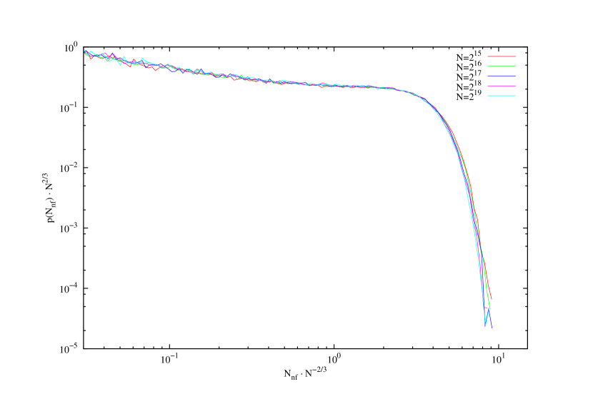
Figure 1: Probability distribution of the number $N_{nf}$ of non frozen nodes for $k=4$, for different $N\in\{2^{15},\ldots,2^{19}\}$, and scaled with $N^{2/3}$. The data were obtained by using the container method, which determines the frozen core by starting from the nodes with constant functions. 100 000 randomly choosen networks where evaluated for each value of $N$.

However, when this procedure is performed for $k\geq 5$, it fails. Only a small part of all nodes become frozen by starting from the nodes with constant functions.

In order to understand this failure of the procedure for $k\geq 5$, let us consider the deterministic difference equations that describe the stochastic process of the container method as long as all $N_{i}$ are large. We denote with $N(t)$ the total number of nodes in the containers at step $t$. At the beginning we have

$$N\left(0\right) = N$$ (4)

$$N_{0}\left(0\right) = \beta\left(k\right)N$$ (5)

$$N_{i}\left(0\right) = 0$$ (6)

$$N_{k}\left(0\right) = \left(1-\beta\left(k\right)\right)N\,.$$ (7)

During each step, the mean container contents change according to

$$\Delta N\left(t\right) = -1$$ (8)

$$\Delta N_{0}\left(t\right) = -1+\sum_{i>0}\omega_{i}\left(i+1\right)\frac{N_{i+1}\left(t\right)}{N\left(t\right)}$$ (9)

$$\Delta N_{i}\left(t\right) = -i\frac{N_{i}\left(t\right)}{N\left(t\right)}+\left(1-\omega_{i}\right)\left(i+1\right)\frac{N_{i+1}\left(t\right)}{N\left(t\right)}$$ (10)

$$\Delta N_{k}\left(t\right) = -k\frac{N_{k}\left(t\right)}{N\left(t\right)},$$ (11)

as long as $N_{0}>0$. If $N_{0}$ reaches $0$, the process stops. This is valid for sufficiently large networks where the probability that two nodes are connected by more than one edge vanishes. For $N\rightarrow\infty$, one can replace these difference equations by differential equations.

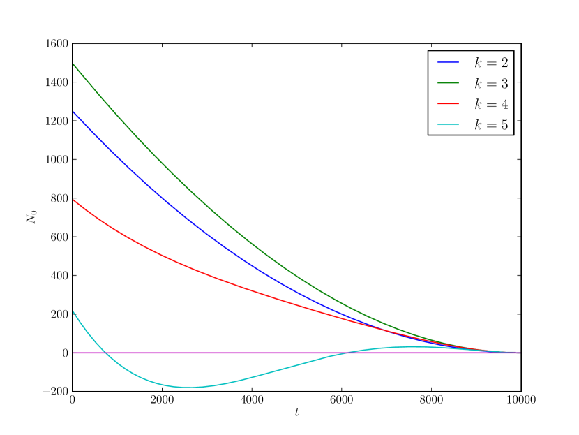
Figure 2: Number of nodes $N_{0}(t)$ in container $C_{0}$ obtained by iterating the deterministic equations (4-11) for different values of $k$ and network size $N=10\,000$. We continued the computation until $t=N$. For $k>4$, the function $N_{0}(t)$ intersects the $x$-axis twice.

Figure 2 shows the number of nodes in container $C_{0}$ for different values of $k$ for a numerical iteration of the deterministic difference equations. For $k=5$, we did not stop the iteration at $N_{0}=0$, but we continued to $t=N$. For $k<5$, $N_{0}$ decreases monotonically from its initial value at $t=0$ to 0 at $t=N$. For $k=5$, $N_{0}$ becomes negative for a value $t/N$ close to 0 and becomes positive again only when $t/N$ is not too far from the value 1. From there, it reaches a local maximum and decreases then again to 0 at $t/N=1$. A similar behavior is found for larger $k$ (not shown).

The fact that $N_{0}$ becomes zero while a large proportion of the network is not yet frozen means that the frozen core cannot be built by starting only from those nodes that have constant functions. In principle, this could also mean that different sets of nodes remain unfrozen for different initial conditions, or that those nodes that freeze for all initial conditions do not always freeze on the same value. However, as we will argue below, the frozen core comprises also for $k\geq 5$ all but of the order $N^{2/3}$ nodes of the network. If we want to interpret the fact that $N_{0}$ first becomes negative and then becomes positive again at a larger $t/N$, we can reason as follows: When we continue freezing inputs and decreasing $N_{0}$ by 1 at each step, even though $N_{0}$ is 0 or negative, we assume that there exist frozen nodes that we have not yet identified, but that we will identify later. This assumption does not lead to a contradiction if during this process enough nodes freeze that $N_{0}$ becomes again positive. The assumption that there exists a large number of frozen nodes that are not frozen by starting from the constant functions, is then proven self-consistent.

When a more general set of update functions is used instead of biased functions, the condition $N_{0}(t)=0$ can have nontrivial solutions already for $k=3$. For a general set of functions [14], the probabilities $\omega_{i}$ that a node with $i+1$ inputs becomes frozen when one of its inputs freezes, can take values different from those for biased functions, Equation (3). For $k=3$, we obtain the following conditions for the existence of a solution $N_{0}(t)=0$ for $t/N<1$:

$$0<\omega_{2} < \frac{1}{3}$$

$$\frac{1}{2}<\omega_{1} < 1-\frac{1}{3\left(1-\omega_{2}\right)}$$

$$1-\beta\left(3\right) = \frac{1}{3\left(1-\omega_{1}\right)\left(1-\omega_{2}\right)}.$$

The third condition is the condition for criticality.

As an aside, we note that if $N_{0}$ becomes negative for critical network, it will also become negative for “frozen” networks as long as the control parameter is not too far away from its critical value. This means that even networks that are in the frozen phase are not necessarily frozen because of constant functions.

On the other hand, there exist sets of update functions where the container method does not fail for any value of $k$. One such set is obtained by only choosing constant and reversible functions, as was done in [18]. Another such set was used in [19], where the process of formation of the frozen core was viewed as an exhaustive bond percolation process. By assuming that the probability that a randomly chosen node is frozen if $l$ of its inputs are frozen does not change during the process, the authors obtained a simpler recursion relation than our difference equations above. This simpler recursion relation is valid for bond percolation, but not for our model with biased functions, where the set of nodes that have already been removed from the system has a different probability distribution of update functions than the set of nodes that are still left in the containers. Therefore, we must keep track of the probability distribution of the different types of functions by monitoring the contents of each container.

Until now, we have focused on the size of the frozen core. For $k<5$ and biased functions, the frozen core can be determined by starting from the constant nodes and determining iteratively all nodes that become frozen because they have frozen inputs. However, the container method does not reflect the real freezing dynamics. Therefore, we studied the freezing process by computer simulations of networks. In order to determine the influence of the nodes with constant functions on the freezing dynamics, we compared the number of frozen nodes obtained from a straightforward computer simulation of the network with the number of nodes that become frozen because their inputs have become frozen, which is the situation considered in the container method. In the first case, all nodes that did not change their state during the remainder of the simulation were considered frozen after the moment when they changed last. The freezing process according to the “container method” was implemented by considering all nodes with constant functions frozen at $t=0$, and by freezing at time $t$ all those nodes that become frozen because one or more of their inputs became frozen at time $t-1$. This amounts to running the container method with a parallel update procedure, where all nodes in container $C_{0}$ are dealt with during the same time step.

Figure 3 shows the result of such a comparison for $k=2,3,4,5$. The final set of frozen nodes is almost the same in both evaluations for $k=2,3,4$, confirming that almost all nodes that become frozen are part of the frozen core. However, the number of nodes that are frozen at a given moment in time is considerably larger when all actually frozen nodes are counted and not only those that have become frozen because of a freezing cascade that begins at nodes with constant functions. The difference between the two simulations becomes larger for larger $k$.

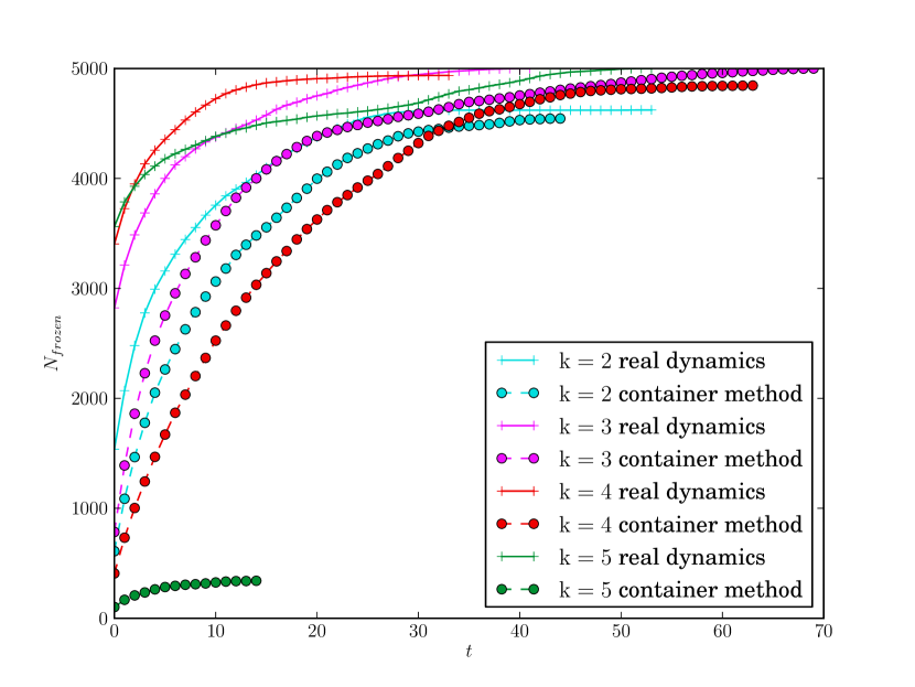
Figure 3: Comparison of the freezing process using real dynamics and the container method with parallel update for four networks with $k\in\left\{2,\ldots,5\right\}$ and $N=5\,000$. For “real dynamics”, a node was assumed to be frozen if it did not change its state any more during the remainder of the simulation. For the “container method”, a node was considered frozen if the freezing of its input(s) caused it to freeze, with the initially frozen nodes being those with constant functions.

In the following sections, we aim at understanding better the actual dynamics of the formation of the frozen core. In particular, we will investigate whether there is a qualitative difference in the freezing dynamics and the nature of the frozen core between networks with $k<5$ and with $k\geq 5$. First, we will present computer simulations that suggest that there is no qualitative difference. Then, we will present an analytical calculation based on mean-field considerations that corrobates this finding.

4 Computer simulations of the dynamics of the formation of the frozen core

Figure 4 shows the proportion of frozen nodes as function of time, for different values of $k$. Each curve is averaged over several 1 000 networks. The network size was $N=2^{14}$, and we found that for networks as large as this the curves do not change any more with increasing $N$. The simulations where performed until an attractor was reached. Nodes that did not change on the attractor were considered as frozen. If no attractor was reached until the end of the simulation $t_{max}=\frac{N}{2}$, we considered a node frozen after its last flip seen in the simulation. This introduces a small finite-size effect, but as mentioned before, our results change very little with $N$ for the values used in these simulations. With increasing $k$, freezing becomes faster, but no qualitative difference can be perceived between the curves for $k<5$ and $k\geq 5$.

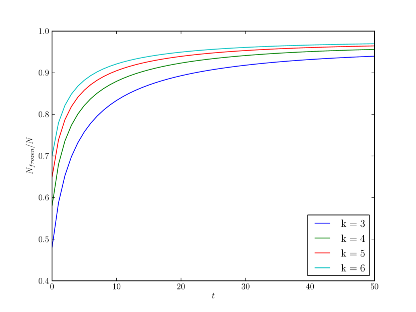
Figure 4: Proportion of frozen nodes as function of time for different values of $k$, averaged over several 1 000 networks with $2^{14}$ nodes.

Next, we investigated whether always the same nodes become frozen. For this purpose, we evaluated the number of nodes that become frozen on all attractors that are reached when starting many times from a random initial state. For $k\geq 5$, the frozen core cannot be obtained by starting from nodes with constant functions, and for this reason we considered it possible that the set of frozen nodes is different for different initial conditions. We also evaluated whether a node that becomes frozen always freezes on the same value and whether the propertion of nodes that freeze at the value 1 is identical to $p$.

Figure 5 shows the proportion of nodes that do not freeze for all 200 initial conditions on the same value, averaged over at least several hundred networks, for $k=5$ and different values of $N$. The date are scaled with $N^{1/3}$. The curves for different $N$ agree well with each other, indicating that only a proportion $\sim N^{-1/3}$ of all nodes do not freeze for all initial conditions, or do not freeze on the same value for all initial conditions.

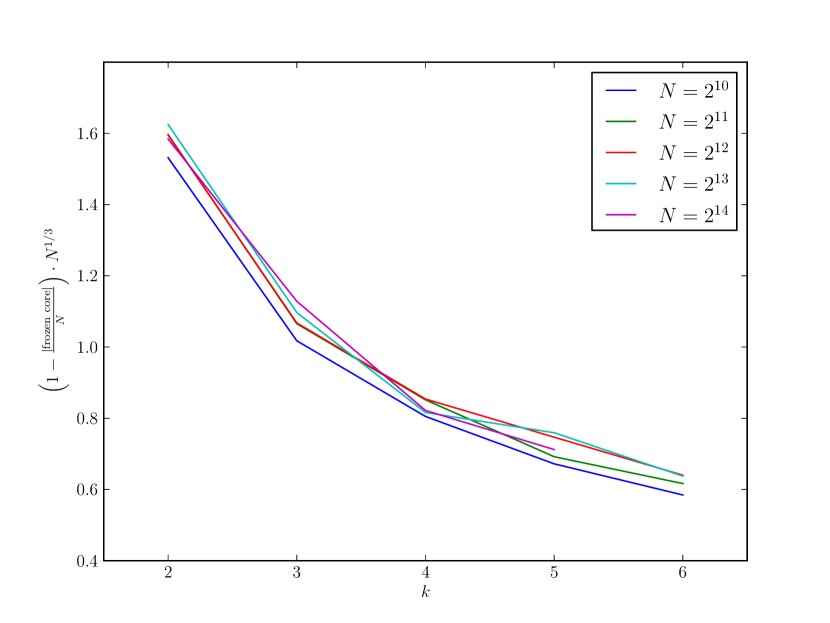
Figure 5: Proportion of nodes that do not always freeze on the same value when starting from 200 different initial conditions, for $k=5$ and different network size $N$. The data are averaged over at least several hundred networks and are scaled with $N^{1/3}$.

Figure 6 shows the proportion of nodes that freeze on the value 1 (which is the minority bit), divided by $p$. This ratio approaches 1 from below with increasing $N$. The larger $k$, the large is the deviation from 1. These data show that it is more likely that a node freezes on its majority bit when the network is smaller and $k$ is larger. The reason for this may be that for larger $k$ and smaller $N$ the networks contain more short connection loops from a node to itself. If such loops are frozen, their nodes have to be insensitive to changes of inputs that are not part of the loop. This means that the output of a node on the loop must be identical for approximately $2^{k-1}$ different input states, i.e., for half the input states. Due to the smallness of $p$, this output must be the majority bit.

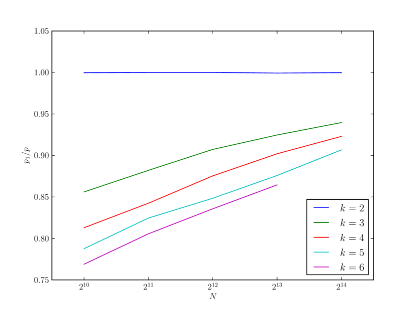
Figure 6: Proportion of nodes that freeze on the minority bit 1, divided by $p$, as a function of $N$ and averaged over at least several hundred networks, for different values of $k$.

Last, we evaluated the histogram of the number of nodes that flip at a given moment in time when the network is not yet on an attractor. When no attractor could be identified during the simulation time $N/2$, the last state was assumed to be a fixed point. Figure 7 shows the data obtained for $N=2^{14}$ and for different values of $k$. Again, no qualitative change can be seen between values $k<5$ and $k\geq 5$. With increasing $k$, the nodes freeze earlier, and the curves become lower. The peak at the end of the curves is a finite-size effect. Its position scales with $N$. Before the finite-size effect sets in, the curves appear to follow a power law with an exponent $-2$. We will confirm this exponent in the next section, where we perform a mean-field calculation.

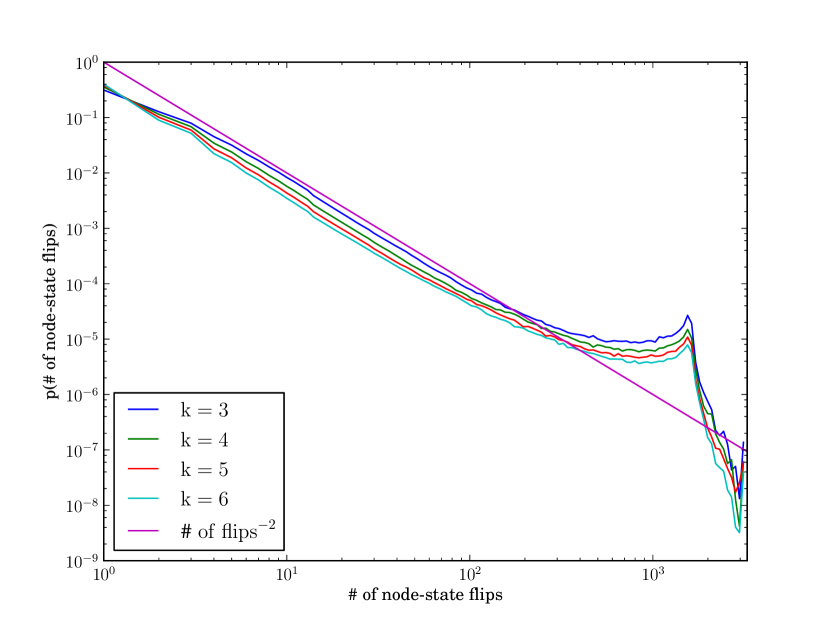
Figure 7: Number of node-state flips on the transient from initial state to the attractor, averaged over at least several thousend networks of size $N=2^{14}$.

5 Mean-field theory for the formation of the frozen core

In the following, we perform a mean-field calculation for the formation of the frozen core. This calculation evaluates the probability that a nodes flips in a given time step in dependence of the probability that at least one of its inputs has flipped in the previous time step. This calculation neglects correlations between nodes and between flips of the same node at different times. It is therefore valid only when the time is short enough so that the network has not yet reached a periodic attractor. Since the most important relevant loop in a critical Random Boolean Network has a size of the order of $N^{\frac{1}{3}}$ [13], we thus expect finite-size effects to become visible after of the order of $N^{\frac{1}{3}}$ time steps.

We start from a random initial state, where each node is in the state 1 with a probability $p$. After the first time step, each node takes the value that is prescribed by its Boolean function, given the values of the inputs. The probability that this is an other state as before is $2p\left(1-p\right)=F_{0}$. (This is the probability that the node flips from 0 to 1 or from 1 to 0.) In each of the following steps, a node can only flip if one of its inputs has flipped in the previous time step. We denote by $F_{t}$ the proportion of nodes that flip in time step $t$. The probabilty that at least 1 input of a node has flipped at time $t$, is $\left(1-\left(1-F_{t}\right)^{k}\right)$. From this, we obtain

$$F_{t+1}=\left(1-\left(1-F_{t}\right)^{k}\right)F_{0}\,.$$ (12)

The fixed points of this recursion relation are given by the condition $F^{\star}=\left(1-\left(1-F^{\star}\right)^{k}\right)F_{0}$. The function on the right-hand side has its maximum slope at $F^{\star}=0$. This slope is smaller than 1 when $k$ is smaller than $1/(2p(1-p))$. In this case, the map (12) converges to the fixed point 0, which means that all nodes become frozen. In the opposite case, there is a stable fixed point at a nonzero value of the node flip rate. At the boundary, the system is critical, with the node-flip activity approaching zero marginally slowly. This is equivalent to the condition formulated in Equation (1).

A Taylor expansion of the map (12) close to $F_{t}=0$ in a critical network with $F^{c}_{0}=F_{0}=2p(1-p)=1/k$ gives

$$F_{t+1} = \left(1-\left(1-F_{t}\right)^{k}\right)F^{c}_{0}$$

$$= F_{t}-\frac{k\left(k-1\right)}{2}F_{t}^{2}F^{c}_{0}+\mathcal{O}\left(F_{t}^{3}\right)\,.$$

From this, we obtain

$$\Delta F_{t+1}=F_{t+1}-F_{t}\approx-\frac{k\left(k-1\right)}{2}F_{t}^{2}F^{c}_{0}$$

Transforming this into a differential equation and integrating it leads to

$$F\left(t\right)=\frac{2}{\left(k-1\right)t}\,.$$ (13)

This means that the number of flipping nodes decreases for large times as $1/t$. The number of nodes that flip at time $t$ for the last time is proportional to $-\dot{F}(t)$, which in turn is proportional to $1/t^{2}$. We have thus obtained an explanation for the exponent $-2$ found in Figure 7.

In order to assess the quality of our mean-field calculation, we evaluated the number of nodes that flip at each time step in real critical networks. Figure 8 shows the results obtained for differerent network sizes $N$, for $k=2$, averaged over 10 000 networks. In addition to the simulation results, this graph shows also the mean-field result and Equation 13. The graph is very similar for larger values of $k$.

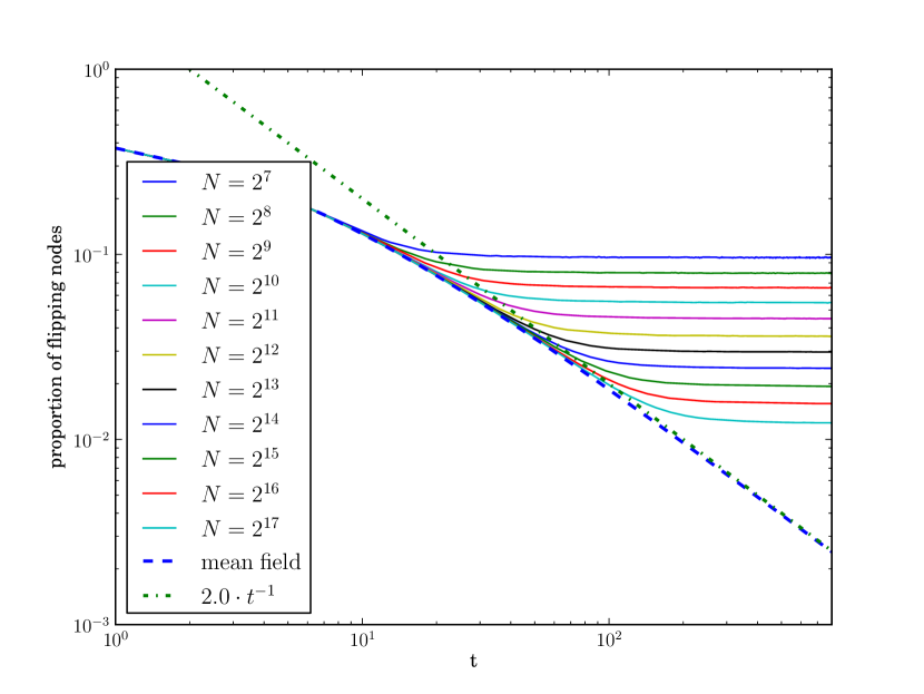
Figure 8: Comparison of mean field theory and simulation. The figure shows the proportion of flipping nodes for differerent network sizes $N$, for $k=2$, averaged over 10 000 networks. In addition to the simulation results, this graph shows also the mean-field result and the power law (13) with the slope $-1$.

One can see that up to a cutoff time the simulation data agree perfectly with the mean-field calculation. An evaluation of the cutoff time reveals that it scales as $N^{\frac{1}{3}}$, which is in agreement with our estimate of finite size effects at the beginning of this section. After this time, the network has reached its stationary activity level.

So far, the mean-field theory tells us only that almost all nodes become frozen in a critical network, and that the time dependence of the number of frozen nodes agrees with computer simulations. However, more information can be extracted from the mean-field theory by realizing that the recursion for $F_{t}$ remains identical if $F_{t}$ is interpreted to be the normalized Hamming distance between two replicas of the same network that are initiated in random initial states where each node is 1 with probability $p$ and 0 with probability $1-p$. The normalized Hamming distance is defined as the proportion of nodes the states of which differ in the two replicas. The probability that the state of a node is different in the two replicas at time $t$ is identical to the probability that the state of at least one input was different at time $t-1$, multiplied by the probability that a different input leads to a different output. This leads again to the recursion relation (12). As shown for instance in [20], the long-term behavior of the Hamming distance can be used as a criterion for deciding whether a network is in the frozen or chaotic phase. At the boundary, it is critical. For critical networks, the normalized Hamming distance goes to zero, which means that almost all nodes are frozen on the same value when the network is started in two different random initial states. Now, if for any two initial states almost all nodes freeze on the same value, almost all nodes are part of the frozen core. This analytical consideration confirms what was suggested by the simulation results shown in Figure 5.

6 Conclusion

We have presented an analysis of the dynamics of the formation of frozen nodes in critical random Boolean networks. We implemented networks with biased functions and studied the dependence of the properties of the frozen core on the in-degree $k$. We found that for $k>4$ the frozen core cannot be obtained by starting from the nodes with constant functions and by determining iteratively all nodes that become frozen because some or all of their inputs have become frozen. When other sets of update functions are used, this effect can already occur at $k=3$. Nevertheless, our computer simulations of the freezing process suggested that there is no qualitative difference between the properties of the frozen core for $k\leq 4$ and $k>4$. By performing a mean-field calculation for the number of nodes that flip as a function of time, we could calculate two power laws that are observed in the computer simulations, and we could show that the dynamics of the formation of the frozen core can be captured correctly by neglecting correlations between nodes and between subsequent flips of the same node.

Furthermore, our computer simulations showed that irrespective of the initial state always the same nodes freeze, apart from a fraction proportional to $N^{-1/3}$, and that these nodes always freeze in the same state. For $k\leq 4$, this result is obtained by starting from nodes with constant functions. For $k>4$, this result points to the existence of large groups of nodes that remain frozen once they are fixed on specific values. We confirmed this observation with a mean-field calculation.

Due to the universality of critical behavior, we expect our results to hold for random Boolean networks with other sets of Boolean functions apart from biased functions, and for networks where not all nodes have the same in-degree $k$, as long as the second moment of the distribution of $k$ values is finite [21].

To conclude, viewing the freezing process of critical random Boolean networks as an avalanche that starts at nodes with constant functions, is an unnecessary limitation that does not capture the universality of the freezing process. Rather, as revealed by mean-field theory, freezing is ultimately due to the insufficient sensitivity of the nodes to changes in their inputs. A critical network with biased functions and a large value of $k$ contains few constant functions, but its value of $p$ is so small that the number of node-state flips decreases fast, and so does the difference between two replicas of the same network.

References

References

- [1] Stuart Kauffman, Carsten Peterson, Bjørn Samuelsson, and Carl Troein. Random Boolean network models and the yeast transcriptional network. Proc. Natl. Acad. Sci. U.S.A., 100:14796, 2003.
- [2] Stuart A. Kauffman. Metabolic stability and epigenesis in randomly constructed genetic nets. J. Theor. Biol., 22:437–467, January to March 1969.
- [3] S. Bornholdt. Less is more in modeling large genetic networks. Science, 310(5747):449, 2005.
- [4] B. Drossel. Random boolean networks. Reviews of nonlinear dynamics and complexity, pages 69–110, 2008.
- [5] Bernard Derrida and Yves Pomeau. Random networks of automata: a simple annealed approximation. Europhys. Lett., 1(2):45–49, January 1986.
- [6] Bernard Derrida and Dietrich Stauffer. Phase transitions in two dimensionalKauffman cellular automata. Europhys. Lett., 2(10):739–745, November 1986.
- [7] Maximo Aldana-Gonzalez, Susan Coppersmith, and Leo P. Kadanoff. Boolean dynamics with random couplings. In Ehud Kaplan, Jerrold E. Mardsen, and Katepalli R. Sreenivasan, editors, Perspectives and Problems in Nonlinear Science, A celebratory volume in honor of Lawrence Sirovich, pages 23–89. Springer Applied Mathematical Sciences Series, Springer Verlag, New York, May May 2003.
- [8] Henrik Flyvbjerg. An order parameter for networks of automata. J. Phys. A, 21:L955, 1988.
- [9] Henrik Flyvbjerg and N. J. Kjær. Exact solution of Kauffman’s model with connectivity one. J. Phys. A, 21:1695, 1988.
- [10] Ugo Bastolla and Giorgio Parisi. Relevant elements, magnetization and dynamical properties in Kauffman networks. a numerical study. Physica D, 115(3&4):203, May 1st 1998.
- [11] Ugo Bastolla and Giorgio Parisi. The modular structure of Kauffman networks. Physica D, 115(3&4):219, May 1st 1998.
- [12] Joshua E. S. Socolar and Stuart A. Kauffman. Scaling in ordered and critical random Boolean networks. Phys. Rev. Lett., 90:068702, 2003.
- [13] Viktor Kaufman, Tamara Mihaljev, and Barbara Drossel. Scaling in critical random boolean networks. Physical Review E, 72(4):046124, 2005.
- [14] Tamara Mihaljev and Barbara Drossel. Scaling in a general class of critical random boolean networks. Phys. Rev. E, 74(4):046101, Oct 2006.
- [15] S.A. Kauffman. Emergent properties in random complex automata. Physica D: Nonlinear Phenomena, 10(1-2):145–156, 1984.
- [16] U. Paul, V. Kaufman, and B. Drossel. Properties of attractors of canalyzing random boolean networks. Physical Review E, 73(2):026118, 2006.
- [17] Maximo Aldana-Gonzalez, Susan Coppersmith, and Leo P. Kadanoff. Boolean dynamics with random couplings. Perspectives and Problems in Nonlinear Science, pages 23–89, May 2003.
- [18] B. Drossel and F. Greil. Critical boolean networks with scale-free in-degree distribution. Physical Review E, 80(2):026102, 2009.
- [19] B. Samuelsson and J.E.S. Socolar. Exhaustive percolation on random networks. Physical Review E, 74(3):036113, 2006.
- [20] M. Aldana-Gonzalez, S. Coppersmith, and LP Kadanoff. Perspectives and problems in nonlinear science, a celebratory volume in honor of lawrence sirovich ed e kaplan. JE Mardsen and KR Sreenivasan (New York: Springer), 2003.
- [21] D.S. Lee and H. Rieger. Broad edge of chaos in strongly heterogeneous boolean networks. Journal of Physics A: Mathematical and Theoretical, 41:415001, 2008.