Polaronic effects in electron shuttling

Abstract

Shuttle-like mechanism of electron transport through a single level vibrating quantum dot is considered in the regime of strong electromechanical coupling. It is shown that the increment of shuttle instability is a nonmonotonic function of the driving voltage. The interplay of two oppositively acting effects - vibron-assisted electron tunneling and polaronic blockade - results in oscillations of the increment on the energy scale of vibron energy.

I Introduction

The modern trends in miniaturization of electronic devices eventually led to fabrication of single molecular junctions and molecular transistors (see e.g. review PR ). The electric properties of single molecular transistors (SMTs) in many cases are similar to the analogous characteristics of single electron transistors (SETs) fabricated in two-dimensional electron gas. SMTs demonstrate such effects as Coulomb blockade and Coulomb blockade oscillations on gate voltage. The significant difference between SMT and semiconducting SET is that the former can function even at room temperatures that makes them to be very promising basic elements for nanoelectronics.

Another specific feature of molecular transistors is the interaction between electronic and vibrational degrees of freedom. The electron in the process of tunneling through the molecule can excite (and absorb at finite temperatures) molecular vibrational quanta (vibrons) - the phenomenon known as ”phonon-assisted tunneling” GlSh . The opening of inelastic channels results in appearance of additional peaks (side-band peaks) in differential conductance. For weak electron-vibron interaction the magnitudes of inelastic peaks are much smaller then the value of the elastic resonance peak. The situation is changed in the regime of strong electron-vibron interaction when nonperturbative (and, in particular, polaronic) effects determine electron transport through a vibrating molecule (see e.g.PR ).

Polaronic effects are most pronounced in the case when the molecule (quantum dot) is well-separated from the leads and the width, $\Gamma$, of conducting molecular states is small compared to other energy scales (temperature $T$, driving voltage $eV$). In this case the mechanism of electron transport through the vibrating molecule is (inelastic) sequential tunneling via the real polaronic intermediate state. The amplitude of this tunneling is exponentially suppressed since the wave functions of free electron in the leads and polaronic state (Holstein polaron) in the dot are almost orthogonal. This effect (named as Frank-Condon Kch ,Kcha or polaronic Krive blockade) strongly suppresses elastic channel of electron transport and changes the temperature behavior of conductance. Recently, Frank-Condon blockade was observed in experiment of electron tunneling through a suspended single-wall carbon nanotube Leturcq .

A one more novel phenomenon appears for vibrating quantum dot when the matrix element of electron tunneling to the left and to the right lead differently depends on the position of the dot center of mass. This is always the case when the dot (molecule) vibrates in the direction of electron tunneling and then the effect of electron shuttling takes place at finite voltages 2.2 -2.4 . In papers 2.3 ,2.4 the problem of electron shuttling was considered for a model of single level ($\varepsilon_{0}$) vibrating quantum dot weakly coupled to the leads of noninteracting electrons. It was shown that in the regime of weak electromechanical coupling the shuttle instability occurs at bias voltages $eV\geq 2(\varepsilon_{0}+\hbar\omega_{0})$ ($\hbar\omega_{0}$ is the vibron energy) and the increment of instability is $r_{0}\sim(\Gamma_{0}/\hbar)\lambda\lambda_{t}$. Here $\Gamma_{0}$ is the level width, $\lambda$ is the dimensionless electron-vibron interaction constant and $\lambda_{t}=x_{0}/l_{t}$ ($x_{0}$ is the amplitude of zero-point fluctuations of quantum dot, $l_{t}$ is the electron tunneling length). Both coupling constants $\lambda$, $\lambda_{t}$ were assumed to be small in Refs.2.3 ,2.4 .

In the problem of electron shuttling the electron-vibron interaction strength $\lambda(V)$ linearly depends on the driving voltage. Therefore, at sufficiently high voltages the regime of strong electron-vibron interaction ($\lambda\gtrsim 1$) is realized. In this regime polaronic effects could play significant role in electron shuttling. In the present paper we reconsider the problem of shuttle instability for the regime of strong electromechanical coupling.

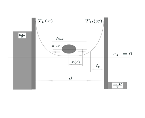
Figure 1: Schematical diagram of Single Electron Transistor (SET) with vibrating quantum dot (QD). Here $\Delta(eV)$ denotes the ”shifted” (due to polaronic shift) bias voltage-dependent fermionic level; $\hbar\omega_{0}$ is the energy of vibrational mode; $T_{L(R)}(x)$ are the coordinate-dependent tunneling amplitudes and $\pm eV/2$ are the chemical potentials of the leads $\varepsilon_{F}=0$. Characteristic distances in the QD: $d$ is the distance (”gap”) between the leads; $l_{t}$ is the tunneling length of the electron in the QD; $\bar{x}(t)$ is average coordinate of the shuttle.

We derived the equation of motion for the shuttle average coordinate $\bar{x}(t)$ assuming only the weak character of dot-lead interaction. It was shown that the increment $r_{s}(V)$ of shuttle instability is a nonmonotonic function of bias voltage with a maximum at $eV_{m}\sim\hbar\omega_{0}(d/x_{0})^{2}$, where $d\gg x_{0}$ is the distance between the leads. The maximum value of the increment is sensitive to value of coupling constant $\lambda_{t}$. The interplay of two effects - the increase of $r_{s}$ caused by the increase of inelastic channels which contribute to the increment when rising the applied voltage and the decrease of $r_{s}$ with the increase of bias voltage caused by polaronic blockade - results in oscillation of $r_{s}$ on small energy scale $\hbar\omega_{0}$.

Our results show that polaronic effects determine the physics of electron shuttling in the case of moderate or strong mechanical damping when the transition to a shuttle-like regime of electron transport is possible only at sufficiently high bias voltages.

II The Model

Our starting point is the model of vibrating quantum dot weakly coupled to the leads of noninteracting electrons. This model was repeatedly considered in the literature for the problem of electron transport in molecular transistors (see e.g.PR and referencies therein). We expand this model to the problem of electron shuttling 2.2 by taking into account the explicit dependence of tunneling amplitude on the center of mass coordinate of quantum dot.

For simplicity we will study the case of a single level (with the energy $\varepsilon_{0}$) quantum dot coupled to a single vibronic mode (with the energy $\hbar\omega_{0}$). The total Hamiltonian of our system is

$$\hat{H}=\sum_{j=L,R}\hat{H}_{l}^{(j)}+\hat{H}_{d}+\sum_{j=L,R}\hat{H}_{t}^{(j)}$$ (1)

where

$$\hat{H}_{l}^{(j)}=\sum_{k}(\varepsilon_{k}-\mu_{j})\hat{a}_{kj}^{+}\hat{a}_{kj}$$ (2)

is the standard Hamiltonian of noninteracting electrons ($\varepsilon_{k}$) in the left ($j=L$) and right ($j=R$) leads, $\mu_{j}$ is the corresponding chemical potential: $\mu_{L}-\mu_{R}=eV$ ( $V$ is the driving voltage); $\hat{a}_{kj}^{+}$ ($\hat{a}_{kj}$) are the creation(destruction) operators. The Hamiltonian of vibrating quantum dot takes the form (see e.g.2.5 )

$$\hat{H}_{d}=\varepsilon_{0}\hat{c}^{+}\hat{c}-\varepsilon_{i}(\hat{b}^{+}+\hat{b})\hat{c}^{+}\hat{c}+\hbar\omega_{0}\hat{b}^{+}\hat{b}\,,$$ (3)

where $\varepsilon_{i}$ is the characteristic energy of electron-vibron interaction (see below), $\hat{c}^{+}$($\hat{c}$) and $\hat{b}^{+}$($\hat{b}$) are fermionic and bosonic creation (destruction) operators with commutation relations $\{\hat{c},\hat{c}^{+}\}=1$; $[\hat{b},\hat{b}^{+}]=1$. The tunneling Hamiltonian is

$$\hat{H}_{t}^{(j)}=\sum_{k}\left[\hat{t}_{j}(\hat{X}_{c.m.})\hat{a}_{kj}^{+}\hat{c}+h.c.\right]\,.$$ (4)

In Hamiltonian Eq.(4) we take into account the dependence of tunneling amplitude $t_{j}$ on the center of mass coordinate $X_{c.m.}$ of quantum dot. In quantum description the coordinate $X_{c.m.}$ becomes an operator

$$\frac{\hat{X}_{c.m.}}{x_{0}}=\hat{X}=\frac{1}{\sqrt{2}}\left(\hat{b}^{+}+\hat{b}\right)\,;\ \hat{P}=\frac{i}{\sqrt{2}}\left(\hat{b}^{+}-\hat{b}\right)\,;$$ (5)

where $x_{0}=\sqrt{\hbar/M\omega_{0}}$, ($M$ is the mass of QD) is the amplitude of zero-point oscillations of quantum dot. In Eq.(5) we defined also the dimensionless momentum operator $\hat{P}$ with the canonical commutation relation $[\hat{X},\hat{P}]=i$. In what follows the tunneling amplitude is model 2.3 by the exponential function

$$\hat{t}_{j}(\hat{X})=t_{0j}\exp(j\lambda_{t}\hat{X}),\qquad j=(L,R)\equiv(-,+)\,.$$ (6)

Here $\lambda_{t}\equiv x_{0}/l_{t}$ and $l_{t}$ is the tunneling length.

Notice that electron-vibron interaction term in Eq.(3) in our model originates from the electrostatic interaction of charge density on the dot with the electrostatic potential produced by the leads 2.3 . It is convinient to characterize this interaction by the dimensionless bias voltage-dependent coupling constant

$$\lambda=\frac{\sqrt{2}\varepsilon_{i}}{\hbar\omega_{0}}=r_{d}\frac{eV}{2\hbar\omega_{0}}\,,\qquad r_{d}=\frac{2x_{0}}{d}\ll 1$$ (7)

($V$ is the bias voltage, $d$ is the distance between the leads). We use the notations usually accepted in the literature on molecular transistors. Notice that our notations for the coupling constants differ from Refs.2.2 ; 2.3 ; 2.4 .

The problem of electron shuttling in the model Eqs.(1)- (3) was studied in Refs.2.3 ; 2.4 for the case of weak electromechanical coupling (in our notations: $\lambda\ll 1$, $\lambda_{t}\ll 1$). In molecular transistors the electron-vibron interaction can be strong $\lambda\gtrsim 1$ (see e.g. PR ). Here we reconsider the problem of shuttle instability 2.3 in the regime of strong coupling.

To study electron transport in the presence of polaronic effects ($\lambda\gtrsim 1$) it is convenient to use unitary transformation (see e.g.2.5 ) which eliminates electron-vibron interaction term in the dot Hamiltonian Eq.(3). Shuttle instability results in appearance of classical time-dependent coordinate $\bar{x}(t)$ of quantum dot. It means that bosonic operators $\hat{b}$ and $\hat{b}^{+}$ acquire $c$-number part $\alpha(t)$:

$$\hat{b}=\alpha(t)+\hat{\tilde{b}}\,;\ \hat{b}^{+}=\alpha^{*}(t)+\hat{\tilde{b}}^{+}\,,$$ (8)

here $\hat{\tilde{b}}^{+}$($\hat{\tilde{b}}$) are the bosonic creation(destruction) operators, which describe quantized vibron modes $\langle\hat{\tilde{b}}\rangle=\langle\hat{\tilde{b}}^{+}\rangle=0$ ($\langle\ldots\rangle$ denotes the thermal average).

We transform total Hamiltonian (1) using the unitary operator (see e.g.PR )

$$\hat{U}=\exp(i\lambda\hat{p}\hat{n})\,,\,\hat{n}=\hat{c}^{+}\hat{c}\,,\,\hat{p}=\frac{i}{\sqrt{2}}\left(\hat{\tilde{b}}^{+}-\hat{\tilde{b}}\right)\,.$$ (9)

The unitary transformed Hamiltonian takes the form

$$\hat{\tilde{H}}=\hat{U}\hat{H}\hat{U}^{-1}=\varepsilon(t)\hat{c}^{+}\hat{c}+\hbar\omega_{0}\hat{b}^{+}\hat{b}+\sum_{j=L,R}\hat{\tilde{H}}_{t}^{(j)}+\sum_{j=L,R}\hat{\tilde{H}}_{l}^{(j)}$$ (10)

where $\varepsilon(t)=\varepsilon_{0}-[\lambda\bar{x}(t)+\lambda^{2}/2]\hbar\omega_{0}$, $\bar{x}(t)=\sqrt{2}Re\alpha(t)$. The time-independent shift ($\sim\lambda^{2}$) of the dot level is called polaronic shift PR . The transformed tunneling Hamiltonian in Eq.(10) is

$$\hat{\tilde{H}}_{t}^{(j)}=\sum_{k}\left[\hat{t}_{j}(\hat{X}_{t})\hat{a}_{kj}^{+}e^{-i\lambda\hat{p}}\hat{c}+h.c.\right]$$

$$=\bar{t}_{0j}\sum_{k}\left[\hat{t}_{j}(\hat{X}_{t})\hat{a}_{kj}^{+}\hat{V}_{j}^{+}\hat{c}+h.c.\right]\,.$$ (11)

Here $\hat{X}_{t}$ is the transformed coordinate operator $\hat{X}_{t}=\hat{U}\hat{X}\hat{U}^{-1}=\hat{X}+\lambda\hat{n}$ and

$$\hat{V}_{j}=\exp(j\lambda_{t}\hat{X}+i\lambda\hat{p})\,,$$

$$\,\bar{t}_{0j}=t_{0j}\exp(j\frac{\lambda\lambda_{t}}{2})\,,\,j=(L,R)\equiv(-,+)\,.$$ (12)

III Equations of motion

The Heisenberg equations of motion for dimensionless operators of coordinate $\hat{X}$ and momentum $\hat{P}$

$$\hat{X}=\frac{1}{\sqrt{2}}\left(\hat{b}^{+}+\hat{b}\right)=\bar{x}(t)+\hat{x}\,,$$

$$\qquad\hat{P}=\frac{i}{\sqrt{2}}\left(\hat{b}^{+}-\hat{b}\right)=\bar{p}(t)+\hat{p}\,.$$ (13)

(where $\bar{x}(t)=\sqrt{2}Re\alpha(t)$, $\bar{p}(t)=\sqrt{2}Im\alpha(t)$ ) can be represented in the form of Hamilton equations

$$\frac{d\hat{X}}{dt}=\frac{1}{\hbar}\frac{\partial\hat{H}}{\partial\hat{P}}\,,\,\,\,\,\frac{d\hat{P}}{dt}=-\frac{1}{\hbar}\frac{\partial\hat{H}}{\partial\hat{X}}\,,$$ (14)

with the Hamiltonian $\hat{H}$ given by the following expression

$$\hat{H}=\frac{\hbar\omega_{0}}{2}\left(\hat{X}^{2}+\hat{P}^{2}\right)+\sum_{j=L,R}\hat{H}_{j}(\hat{X},\hat{p})\,.$$ (15)

Here we denote by $\hat{H}_{j}$ the tunneling Hamiltonian defined by Eq.(II). In our model equations (14) take the form

$$\frac{d\hat{X}}{dt}=\omega_{0}\hat{P}-\lambda\sum_{j=L,R}\hat{J}_{j}(\hat{X},\hat{p})\,,$$

$$\qquad\frac{d\hat{P}}{dt}=-\omega_{0}\hat{X}-\frac{\lambda_{t}}{\hbar}\sum_{j=+/R,-/L}j\hat{H}_{j}(\hat{X},\hat{p})\,,$$ (16)

where $\hat{J}_{L,R}$ are the current operators

$$\hat{J}_{j}=i\frac{\bar{t}_{0j}}{\hbar}\sum_{k}\left[\hat{a}_{kj}^{+}\hat{V}_{j}^{+}\hat{c}-h.c.\right]\,.$$ (17)

These operators satisfy (as it should be) the continuity equation

$$\frac{d\hat{n}}{dt}=\hat{J}_{L}+\hat{J}_{R}\,.$$ (18)

With the help of Eq.(18) we can rewrite the first expression of Eq.(III) in the following form

$$\hat{P}=\omega_{0}^{-1}\frac{d}{dt}\left(\hat{X}+\lambda\hat{c}^{+}\hat{c}\right)\,,$$ (19)

and the second equation in (III) is transformed to

$$\frac{d^{2}}{dt^{2}}\left(\hat{X}+\lambda\hat{c}^{+}\hat{c}\right)+\omega_{0}^{2}\hat{X}=-\frac{\omega_{0}\lambda_{t}}{\hbar}\sum_{j=-/L,+/R}j\hat{H}_{j}(\hat{X},\hat{p})\,,$$ (20)

where $\hat{p}=\hat{P}-\bar{p}(t)$.

To make the operator equations (Eq.(III) or Eqs.(19)), (20) complete we have to write down the equations of motion for fermionic operators $\hat{a}_{kj}$($\hat{a}_{kj}^{+}$) and $\hat{c}$($\hat{c}^{+}$). These equations

$$\frac{d\hat{a}_{kj}}{dt}=-i(\varepsilon_{k}-\mu_{j})\hat{a}_{kj}(t)-i\bar{t}_{0j}\hat{V}_{j}^{+}(t)\hat{c}(t)\,,$$ (21)

$$\frac{d\hat{c}}{dt}=-i\varepsilon(t)\hat{c}(t)-i\sum_{k,j=L,R}\bar{t}_{0j}\hat{V}_{j}(t)\hat{a}_{kj}(t)\,$$ (22)

are linear and they can be readily solved (the equations of motion for creation operators are obtained from Eqs.(21),(22) simply by taking Hermitian conjugation). We will follow Refs.2.3 and find the solution of Eqs.(21),(22) in the so called ”wide band approximation”(”WBA”)(see e.g. WBA ). The only difference of our system of equations (21),(22) from the corresponding one in Ref.2.3 is the presence in our case bosonic operator factors $\hat{V}_{j}$ and $\hat{V}_{j}^{+}$. Formally, these factors make the level width $\hat{\Gamma}$ (see the definition below in Eq.(24), which appears in Eq.(22) after substituting in this equation the solution of Eq.(21), to be an operator as well. The dynamical equation for the dot level operator $\hat{c}$ in WBA takes a simple form

$$\frac{d\hat{c}}{dt}=-i\left[\varepsilon(t)-i\frac{\hat{\Gamma}(t)}{2}\right]\hat{c}(t)$$

$$-i\sum_{k,j=L,R}\bar{t}_{0j}\hat{V}_{j}(t)\hat{a}_{kj}(0)e^{-i(\varepsilon_{k}-\mu_{j})t}\,,$$ (23)

where

$$\frac{1}{2}\hat{\Gamma}(t)=\sum_{j=L,R}\Gamma_{0j}\hat{V}_{j}(t)\hat{V}_{j}^{+}(t)\,.$$ (24)

Here $\Gamma_{0j}=2\pi\rho_{j}|\bar{t}_{0j}|^{2}$ and $\rho_{j}$ is the density of states in the $j=L,R$ electrode ($\rho_{j}$ is assumed to be energy independent in the wide band approximation).

To proceed further we have to make additional simplifications. Our purpose in this section is to derive the equation of motion for the average coordinate in the presence of fluctuations. Notice that in the Hamiltonian Eq.(10) electron-vibron interaction appears only in the tunneling term which for a weak tunneling can be treated perturbatively. In perturbation theory on the bare level widths $\Gamma_{0j}$ vibrons are decoupled from fermions and when evaluating averages of the products of fermion ($\hat{F}$) and boson ($\hat{B}$) operators we can use the decoupling procedure $\,\langle\hat{F}\hat{B}\rangle\backsimeq\langle\hat{F}\rangle_{\tilde{H}_{f}+\tilde{H}_{t}}\langle\hat{B}\rangle_{\tilde{H}_{b}}\,.$ The averages of fermion operators are taken with ”fermionic” part of the total transformed Hamiltonian (including the tunneling part) and averages of boson operators are calculated with the quadratic Hamiltonian of nonointeracting vibrons $\hat{\tilde{H}}_{b}=\hbar\omega_{0}\hat{\tilde{b}}^{+}\hat{\tilde{b}}$. This decoupling procedure is the starting point of calculations in many papers dealing with the polaronic effects in electron transport in molecular junctions (see e.g. review PR and referencies therein).

The linear equation (III) can be formally solved (using time-ordering procedure) for the operator level width $\hat{\Gamma}(t)$. However the closed equation for the average coordinate $\bar{x}(t)$ can be obtained only in perturbation theory on $\Gamma_{0j}$. In Ref.2.4 such equation was obtained in the limit of weak electromechanical coupling $\lambda\ll 1$, $\lambda_{t}\ll 1$. Here we derive the equation for classical coordinate $\bar{x}(t)$ valid also for the regime of strong electron-vibron coupling $\lambda\gtrsim 1$.

In perturbation theory on the bare level width $\Gamma_{0j}$ we can neglect the time dynamics of the level width and replace $\hat{\Gamma}(t)$ by constant $\Gamma_{0}=\Gamma_{0L}+\Gamma_{0R}$. It is convinient in what follows to represent ”vertex” operator $\hat{V}_{j}$ as a product of classical $T_{j}\{\bar{x}(t)\}$ and quantum $\hat{Q}_{j}$ parts $\hat{V}_{j}=T_{j}(t)\hat{Q}_{j}$

$$\hat{T}_{j}(t)=\exp[j\lambda_{t}\bar{x}(t)]\,,\,\hat{Q}_{j}(\hat{x},\hat{p})=\exp(j\lambda_{t}\hat{x}+i\lambda\hat{p})\,,$$

$$\,j=(L,R)\equiv(-,+)\,$$

In the discussed approximation the solution of Eq.(III) takes the form

$$\hat{c}(t)=-i\sum_{k,j=L,R}\bar{t}_{0j}\hat{a}_{kj}(0)e^{-i(\varepsilon_{k}-\mu_{j})t}$$

$$\cdot\int_{0}^{t}dt_{1}T_{j}(t)\hat{Q}_{j}\exp\left\{i\int_{t_{1}}^{t}dt_{2}\left[\varepsilon_{k}-\mu_{j}-\varepsilon(t_{2})+\frac{i}{2}\Gamma_{0}\right]\right\}\,.$$

The equation of motion for the classical coordinate $\bar{x}(t)$ in perturbation theory on $\Gamma_{0j}$ can be readily obtained from the exact operator equation (20) by taking the average and using the discussed above ”fermion-boson” factorization procedure

$$\frac{d^{2}}{dt^{2}}\left[\bar{x}(t)+\lambda N\{\bar{x}(t)\}\right]+\omega_{0}^{2}\bar{x}(t)=-\frac{\omega_{0}\lambda_{t}}{\hbar}\sum_{j=_{+/R}^{-/L}}jH_{j}\left\{\bar{x}(t)\right\}\,,$$ (27)

where

$$N\{\bar{x}(t)\}=\langle\hat{c}^{+}(t)\hat{c}(t)\rangle\,,\qquad H_{j}\left\{\bar{x}(t)\right\}=\langle\hat{H}_{j}(\hat{X},\hat{p})\rangle\,\\$$

It is useful to rewrite Eq.(27) in terms of a new variable $\bar{x}_{v}(t)=\bar{x}(t)+\lambda N\{\bar{x}(t)\}$. Notice that according to Eqs.(II),(III) both quantities in Eq.(27) - averaged tunneling Hamiltonian $H_{j}$ and the level occupation number $N\{\bar{x}(t)\}$ - are proportional to the bare level width $H_{j},N\{\bar{x}(t)\}\propto\Gamma_{0j}$. Since Eq.(27) is derived in the Born approximation (up to the second order in the tunneling amplitude) we can replace $\bar{x}(t)$ by $\bar{x}_{v}(t)$ in the averaged quantities. Then Eq.(27) for the variable $\bar{x}_{v}(t)$ (shifted coordinate) takes the form of the Newton’s equation derived in Ref.2.4

$$\frac{d^{2}}{dt^{2}}\bar{x}_{v}(t)+\omega_{0}^{2}\bar{x}_{v}(t)=\bar{F}_{q}\{\bar{x}_{v}(t)\}\,,$$ (28)

where

$$\bar{F}_{q}\{\bar{x}(t)\}=\lambda\omega_{0}^{2}N\{\bar{x}(t)\}-\frac{\omega_{0}\lambda_{t}}{\hbar}\sum_{j=_{+/R}^{-/L}}jH_{j}\left\{\bar{x}(t)\right\}\,$$ (29)

This equation in the limit $\lambda\ll 1$, $\lambda_{t}\ll 1$, when we can omit operator factors ($\hat{Q}_{j}$) in the vertex function $\hat{V}_{j}$, exactly coincides with the corresponding equation for the coordinate of ”classical” shuttle (see Refs.2.3 ; 2.4 ). One can analyze shuttle instability by using either Eq.(27) or Eq.(28). The only difference is the starting (equilibrium) position of the shuttle. This is $\bar{x}=0$ for Eq.(27) and $\,\bar{x}_{v}=\lambda N\neq 0$ for Eq.(28) (see Ref.2.4 ). We will use Eq.(27).

IV The increment of shuttle instability

The conditions for a shuttle instability can be found by analyzing linearized equation of motion. We will follow Ref.2.4 where these conditions were obtained for the regime of weak electromechanical coupling. The linear integral-differential equation for the shuttle coordinate $\bar{x}(t)$ in the dimensionless units ($t\rightarrow\omega_{0}t$, energy scale is $\hbar\omega_{0}$) reads (see Appendix)

$$\frac{d^{2}}{dt^{2}}\bar{x}(t)+\bar{x}(t)=-\sum_{j=_{+/R}^{-/L}}\frac{\bar{\Gamma}_{0j}}{2\pi}\sum_{l=-\infty}^{+\infty}F_{lj}(\beta)$$

$$\cdot\int_{-\infty}^{+\infty}d\varepsilon f_{j}(\varepsilon)\left\{2Im\left[X_{lj}(\varepsilon,t)\right]\left|\lambda G_{lj}^{(+)}(\varepsilon)-j\lambda_{t}\right|^{2}\right\}\,$$

In Eq.(IV) the following notations are introduced: $\,\bar{\Gamma}_{0j}=\Gamma_{0j}\exp(j\lambda\lambda_{t})$

$$X_{lj}(\varepsilon,t)=\int_{0}^{t}d\tau\bar{x}(\tau)$$

$$\cdot\exp\left\{i\left[(\varepsilon-\mu_{j})-(\Delta-l)+i\frac{\Gamma_{0}}{2}\right](t-\tau)\right\}\,,$$ (31)

and

$$G_{lj}^{(\pm)}(\varepsilon)=\frac{1}{(\varepsilon-\mu_{j})-(\Delta-l)\pm i\Gamma_{0}/2}\,$$ (32)

where $\Delta=\varepsilon_{0}-\lambda^{2}/2\,$ is the polaronic shift. Vibrational degrees of freedom result in Franck-Condon factors

$$F_{lj}(\beta)=\exp[-(\lambda^{2}-\lambda_{t}^{2})(1+2n_{b})]\left|\frac{\lambda+j\lambda_{t}}{\lambda-j\lambda_{t}}\right|^{l}$$

$$\cdot I_{l}(2|\lambda^{2}-\lambda_{t}^{2}|\sqrt{n_{b}(1+n_{b})})e^{-\beta l/2}\,$$ (33)

Here $I_{l}(x)$ is the modified Bessel function of the second kind and $n_{b}=1/(\exp\beta-1)\,$, ($\beta=\hbar\omega_{0}/k_{B}T\,$), $f_{j}(\varepsilon)=1/[\exp(\beta(\varepsilon-\mu_{j}))+1]$ are Bose-Eistein and Fermi-Dirac distribution functions. Remind that all energies in above expressions are dimensionless (in the units of $\hbar\omega_{0}$). In the limit $\lambda_{t}=0$ the vibron-induced correlation factor Eq.(IV) coincides with the well-known in the literature expression (see e.g. Refs.(2.5 ; LMcK ).

The solution of Eq.(IV) with the initial condition $\bar{x}(0)=0$ is

$$\bar{x}(t)=A_{0}e^{r_{s}t}\sin(t)\,.$$ (34)

where $A_{0}$ is an arbitrary constant and

$$r_{s}=\sum_{j=_{+/R}^{-/L}}\frac{\bar{\Gamma}_{0j}}{8}\sum_{l=-\infty}^{+\infty}F_{lj}(\beta)(\lambda-j\lambda_{t})^{2}f_{j}(\Delta-l+1)$$

$$-\sum_{j=_{+/R}^{-/L}}\frac{\bar{\Gamma}_{0j}}{8}\sum_{l=-\infty}^{+\infty}F_{lj}(\beta)(\lambda+j\lambda_{t})^{2}f_{j}(\Delta-l-1)\,$$

is the dimensionless increment (when $r_{s}>0$) of shuttle instability. Our purpose here is to find conditions (driving voltage) for the realization of shuttle motion in the presence of strong electron-vibron interaction.

For a weak electromechanical coupling $\lambda\ll 1$ , $\lambda_{t}\ll 1$ we can neglect quantum and thermodynamical fluctuations of vibrons (they are of higher orders on coupling constants) and omit all terms in the right-hand side of Eq.(IV) but $l=0$. In this limit $\Delta\simeq\varepsilon_{0}$, $\bar{\Gamma}_{0j}\simeq\Gamma_{0j}$, $F_{0j}\simeq 1$ and Eq.(IV) is transformed to the corresponding equation of Refs.2.3 ; 2.4 . The increment Eq.(IV) in this case coincides with the one found earlier Ref.2.4

$$r_{s}^{(0)}=\sum_{j=_{+/R}^{-/L}}\frac{\bar{\Gamma}_{0j}}{8}(\lambda-j\lambda_{t})^{2}f_{j}(\varepsilon_{0}+1)$$

$$-\sum_{j=_{+/R}^{-/L}}\frac{\bar{\Gamma}_{0j}}{8}(\lambda+j\lambda_{t})^{2}f_{j}(\varepsilon_{0}-1)\,$$ (36)

(there is a misprint in Eq.(24) of Ref.2.4 - the sign-changing factor $j$ is missing in the coefficients in front of distrubution functions).

It is qualitatively clear that shuttle instability is most pronounced at low temperatures $\beta\gg 1$ when there are no thermally activated vibrons. At low temperatures shuttle instability results in a sharp (step-like) features in the $I-V$ curve of single electron transistor 2.3 . Finite temperature effects broaden the transition region and at $T\gg\hbar\omega_{0}$ the shuttle instability is less pronounced (nevertheless as far as $r_{s}>0$ the instability results in a strong increase of electric current). In what follows we will consider only low-$T$ effects and (for simplicity) the case of a symmetric junction ($\Gamma_{0L}=\Gamma_{0R}=\Gamma\,,\mu_{L}=-\mu_{R}=eV/2$, we set Fermi energy of the leads $\varepsilon_{F}=0$). At low temperatures the $l>0$ terms in Eq.(IV) are exponentially suppressed in comparison with the negative $l$ (formally, due to the factor $\exp(-l\beta/2)$ since $I_{-l}(x)=I_{l}(x)$ for the integer $l$). Physically, positive $l$ corresponds to vibron absorption - an energetically forbidden process at $T\ll\hbar\omega_{0}$. Negative $l$ describes emission of vibrons and the summation over $l$ at finite bias voltage is limited by a certain $l_{m}$ (see below).

By using the well-known asymptotics of the Bessel function at small arguments $I_{l}(x\rightarrow 0)\sim(z/2)^{l}/l!$ and replacing Fermi distribution functions in Eq.(IV) by the Heaviside theta-functions we obtain the desired formula for the increment ($r_{s}>0$) of shuttle instability

$$r_{s}=\frac{\Gamma\lambda\lambda_{t}}{2}\exp(-\lambda^{2}+\lambda_{t}^{2}-\lambda\lambda_{t})\sum_{l=0}^{l_{m}-1}\frac{(\lambda+\lambda_{t})^{2l}}{l!}$$

$$=\frac{\Gamma\lambda\lambda_{t}}{2(l_{m}-1)!}\exp(\lambda\lambda_{t}+2\lambda_{t}^{2})\Gamma\left(l_{m},(\lambda+\lambda_{t})^{2}\right)\,,$$ (37)

where $\Gamma(\alpha,x)$ is the incomplete gamma function (see e.g. GR ) and

$$l_{m}=\left[\frac{eV}{2}-\left(\varepsilon_{0}-\frac{\lambda^{2}}{2}\right)-1\right]$$ (38)

($[x]$ denotes the integer part of $x$). We find from Eqs.(IV),(38) that in the regime of weak electromechanical coupling the instability occurs at $eV>eV_{c}\simeq 2(\varepsilon_{0}+1)$ 2.3 ,2.4 and the increment $r_{s}(\lambda\ll 1,\lambda_{t}\ll 1)\simeq r_{0}=\Gamma\lambda\lambda_{t}/2\,$ (see Ref.2.4 ) is a linear function of bias voltage. Remind that we consider the case when the uncertainty in the quantum dot initial position due to quantum fluctuations ($\sim x_{0}$) is small compared to the geometrical size $d$ of the junction (that is our parameter $r_{d}=2x_{0}/d\ll 1$, Eq.(7)). In this case at the threshold voltage $V_{c}$ the electron-vibron coupling is small $\lambda(V_{c})=r_{d}(\varepsilon_{0}+1)\ll 1$ (we always can put $\varepsilon_{0}=0$ at the resonance condition) and polaronic effects are not pronounced. Nevertheless there is a small negative correction to the threshold voltage due to polaronic shift $V_{c}=2(\varepsilon_{0}-\lambda^{2}(V_{c})/2+1)$ and the multiplicative renormalization of the bare level width by quantum fluctuations $\,\Gamma\rightarrow\Gamma\exp(-\lambda^{2}+\lambda_{t}^{2}-\lambda\lambda_{t})\simeq\Gamma(1-\lambda^{2}-\lambda\lambda_{t}+\lambda_{t}^{2})\,$, as one can see from Eqs.(IV)(38).

The increment $r_{s}$ is described by Eq.(IV) at bias voltages in the interval $eV_{c}/2<eV/2\leq 2r_{d}^{-2}$. At higher voltages the electron distribution function of the right electrode (biased by $-eV/2$) in Eq.(IV) $f_{R}=1$ and the processes of inelastic electron tunneling to the right bank start to contribute to $r_{s}$. Their contributions according to Eq.(IV) at low temperatures are negative and they could only diminish the increment. We show now that due to polaronic (Franck-Condon) blockade both the ”right” and ”left” contributions at voltages $eV>2r_{d}^{-2}\gg 1$ are exponentially suppressed and shuttle instability takes place in the finite interval of bias volages (we restore here the dimensions)

$$2(\varepsilon_{0}+\hbar\omega_{0})<eV\leq 4\hbar\omega_{0}/r_{d}^{2}\,$$ (39)

The finite series on $l$ in Eq.(IV) can be approximated as follows

$$S_{l}(x)=\sum_{n=0}^{l}\frac{x^{n}}{n!}\simeq\begin{cases}e^{x},\qquad&l\gg x;\cr x^{l}/l!&x\gg l\gg 1.\cr\end{cases}$$ (40)

With the help of asymptotics Eq.(40) we obtain the following formula for $r_{s}$ at $eV\ll r_{d}^{-2}$ (the corresponding electron-vibron coupling ”constant” $\lambda=r_{d}(eV/2)\ll r_{d}^{-1}$)

$$r_{s}\simeq\frac{\Gamma\lambda\lambda_{t}}{2}\exp(\lambda\lambda_{t}+2\lambda_{t}^{2})\,$$ (41)

For a very high biases $eV\gg r_{d}^{-2}$ it is easy to show from Eqs.(IV),(40) (using Sterling’s formula to estimate asymptotics of $l_{m}!$) that $\,r_{s}\propto\exp[-\lambda^{2}(1-\ln 2)/2]\rightarrow 0$ at $\lambda\gg 1$. So we see that the dependence of increment $r_{s}$ on the bias voltage is strongly nonmonotonic with the maximum at $eV\sim r_{d}^{-2}$.

It is interesting to notice here that at the excitation energy $E_{d}\simeq\hbar\omega_{0}(r_{d})^{-2}$ (the corresponding number of excited vibrons $l_{d}\simeq r_{d}^{-2}\gg 1$) the characteristic width, $w$, of the wave function of harmonic oscillator which represents quantum dot in our model (Eq.(3)) is of the order of gap, $d$, between the leads ($w\sim x_{0}\sqrt{\langle\hat{x}^{2}\rangle}\sim x_{0}\sqrt{l_{d}}\sim d$).

The approximation Eq.(40) does not reveal the fine structure (on the $\hbar\omega_{0}$ scale) of the dependence $r_{s}(V)$. On this small energy scale one could expect the appearance of steps each time the additional vibration channel contributes to the increment (see Eq.(38)). At low voltages the steps are slightly modified by the Franck-Condon factors. With the increase of voltage in the regime of strong coupling $\lambda>1$ each additional channel modifies $r_{s}$ by the value of the order (few times smaller) of $r_{s}$ (sharp big steps). However between two sequential steps $r_{s}$ is diminished (due to the $\exp(-\lambda^{2}(V))$ factor in Eq.(IV)) approximately by the same amount. That is on the scale of vibron energy there are oscillations of $r_{s}$. These oscillations are smeared out at temperatures $T\gg\hbar\omega_{0}$.

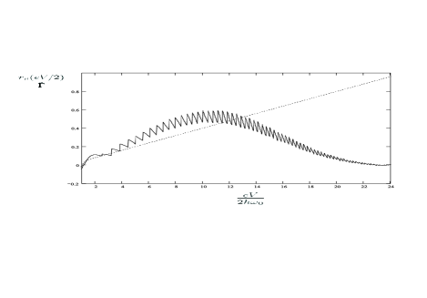
Figure 2: ”Weak” shuttle instability. The increment of shuttle instability (in the units of $\Gamma/\hbar\omega_{0}$) as a function of bias voltage for $\lambda_{t}=x_{0}/l_{t}=0.2$; $r_{d}=x_{0}/d=0.2$ (solid line) and $\beta^{-1}=k_{B}T/\hbar\omega_{0}=0.2$. The dotted line represents the result of Ref 2.4 extended to the region of strong electromechanical coupling.

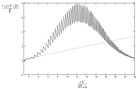
Figure 3: ”Strong” shuttle instability. All parameters are the same as in Fig.2, but for the coupling constant $\lambda_{t}=0.7$.

The dependence $r_{s}(V)$ is plotted in Figs.2,3 for the different values of parameters of our model (for numerical calculations we used the basic Eq.(IV) and put the inverse temperature $\beta=10$). For both figures we set $r_{d}=0.2$, since the further decrease of $r_{d}$ yields the results which practically coincide with Ref.2.4 in the considering region of applied voltages. The dimensionless increment $r_{s}$ of the shuttle instability is measured in the units of dimensionless $\tilde{\Gamma}=\Gamma/\hbar\omega_{0}$ ($eV$ is in the units of $\hbar\omega_{0}$). In Fig.2 we set $\lambda_{t}=r_{d}=0.2$, that corresponds to the case when $2l_{t}\sim d$. In Fig.3 we put $\lambda_{t}=0.7>r_{d}$, that corresponds to the case when $2l_{t}<d$. The straight line on both figures shows the increment for the ”classical” shuttle of Ref.2.4 for the same values of all parameters.

We see from the figures, that, the dependence of increment on bias voltage is strongly nonmonotonic. The increment $r_{s}$ grows until $eV\leq eV_{m}\approx r_{d}^{-2}$ and decreases when $V>V_{m}$. The magnitudes of $r_{s}$ in Fig.3 ($\lambda_{t}=0.7$) are much greater than the ones in Fig.2 ($\lambda_{t}=0.2$). This means, that shuttle instability is very sensitive to the value of tunneling lengths $\lambda_{t}$. So, when $l_{t}\ll d$ ($r_{d}\ll 1$), the greater is $\lambda_{t}$ the stronger is shuttle instability (i.e. it develops on a shorter time scale $\sim r_{s}^{-1}$). In the presence of strong mechanical friction, characterized by phenomenological damping term, $i\gamma_{f}\dot{\bar{x}}(t)$, introduced in Eq.(27), and for $2l_{t}\lesssim d$ (i.e. $r_{d}\lesssim 1$), when $\lambda_{t}\ll 1$, the increment at all voltages could be less then the friction coefficient $r_{s}<\gamma_{f}$. In this case shuttle regime of electron transport is not realized.

V Summary

In this paper we have studied the influence of quantum and thermodynamical fluctuations on shuttle instability. These fluctuations are significant in the case of strong electromechanical coupling that can be realized in electron transport through vibrating quantum dot at high bias voltages.

It was shown that the increment of shuttle instability is a nonmonotonic function of bias voltage $V$ with a maximum at $eV_{m}\sim\hbar\omega_{0}(d/x_{0})^{2}$, which corresponds to the region of strong electron-vibron coupling $\lambda(V_{m})\gg 1$. At higher voltages polaronic blockade suppresses shuttle instability. The maximum value of increment is sensitive to the electromechanical dimensionless coupling constant $\lambda_{t}=x_{0}/l_{t}$ ($l_{t}$ is the electron tunneling length). In the presence of mechanical friction (characterized by phenomenological friction coefficient $\gamma_{f}$) and when $\lambda_{t}\ll 1$ the increment $r_{s}(V)$ at all voltages could be less then friction $r_{s}(V)<\gamma_{f}$ and shuttle regime of electron transport is not realized. In the regime of strong electromechanical coupling $\lambda_{t}\sim 1$, $\lambda\gg 1$ the pumping of energy in mechanical shuttle motion could overcome even strong damping.

We showed that in this regime the increment of shuttle instability strongly oscillates on the energy scale of vibron energy $\hbar\omega_{0}$. If the friction coefficient is comparable with the amplitude of increment oscillations, the small change of bias voltage ($\Delta V\lesssim\hbar\omega_{0}/e$) drastically changes the regime of electron transport through a vibrating quantum dot (from a phonon-assisted tunneling to a shuttle regime of electron transfer and vice-a-versa). One can speculate that reentrant transitions to a shuttle-like regime of electron transport will result in unusual current-voltage characteristics with pronounced negative differential conductance.

VI Acknowledgments

The authors thank S.I.Kulinich for valuable discussions. This work was supported in parts by the Swedish VR and SSF, by the Faculty of Science at the University of Gothenburg through the ”Nanoparticle” Research Platform and by the grant ”Effects of electronic, magnetic and elastic properties in strongly inhomogeneous nanostructures” provided by the National Academy of Sciences of Ukraine. IVK thanks the Department of Physics at the University of Gothenburg for hospitality.

VII The Appendix

To study the shuttle instability we linearize the Eq.(28) ($\lambda\bar{x}(t)\ll 1$, $\lambda_{t}\bar{x}(t)\ll 1$). In the linear approximation we have $T_{j}(\bar{x}(t))=\bar{t}_{0j}(1+j\lambda_{t}\bar{x}(t))$, $j=-/L;+/R$ and $\hat{c}(t)=\hat{c}_{0}(t)+\hat{c}_{1}(t,\bar{x}(t))$, where

$$\hat{c}_{0}(t)=-i\sum_{k,j=L,R}\bar{t}_{0j}\hat{a}_{kj}(0)e^{-i(\varepsilon_{k}-\mu_{j})t}$$

$$\cdot\int_{0}^{t}dt_{1}\hat{Q}_{j}(t_{1})\exp\left\{i\left[\varepsilon_{k}-\mu_{j}-\Delta+\frac{i}{2}\Gamma_{0}\right](t-t_{1})\right\}\,$$

and

$$\hat{c}_{1}(t)=-i\sum_{k,j=-/L,+/R}\bar{t}_{0j}\hat{a}_{kj}(0)e^{-i(\varepsilon_{k}-\mu_{j})t}$$

$$\cdot\int_{0}^{t}dt_{1}\left[j\lambda_{t}\bar{x}(t_{1})+\lambda\int_{t_{1}}^{t}dt_{2}\bar{x}(t_{2})\right]$$

$$\cdot\hat{Q}_{j}(t_{1})\exp\left\{i\left[\varepsilon_{k}-\mu_{j}-\Delta+\frac{i}{2}\Gamma_{0}\right](t-t_{1})\right\}\,$$

Here $\Delta=\varepsilon_{0}-\lambda^{2}/2$ is the polaronic shift.

Then, the linearized force $F_{q}(t)$ in the right-hand side of the Eq.(28) is represented as the sum of two contributions: $F_{q}=F_{0}+F_{1}$, where

$$F_{0}=\lambda\langle\hat{c}_{0}^{+}(t)\hat{c}_{0}(t)\rangle$$

$$-\sum_{k,j=-/L,+/R}j\lambda_{t}\bar{t}_{0j}\langle\hat{Q}_{j}^{+}(t)\hat{a}_{kj}^{+}(0)e^{i(\varepsilon_{k}-\mu_{j})t}\hat{c}_{0}(t)\rangle$$

$$-\sum_{k,j=-/L,+/R}j\lambda_{t}\bar{t}_{0j}\langle\hat{c}_{0}^{+}(t)\hat{a}_{kj}(0)e^{-i(\varepsilon_{k}-\mu_{j})t}\hat{Q}_{j}(t)\rangle\,$$

and

$$F_{1}=-\lambda_{t}\bar{x}(t)\sum_{k,j=L,R}\bar{t}_{0j}\langle\hat{Q}_{j}^{+}(t)\hat{a}_{kj}^{+}(0)e^{i(\varepsilon_{k}-\mu_{j})t}\hat{c}_{0}(t)\rangle$$

$$-\lambda_{t}\bar{x}(t)\sum_{k,j=L,R}\bar{t}_{0j}\langle\hat{c}_{0}^{+}(t)\hat{a}_{kj}(0)e^{-i(\varepsilon_{k}-\mu_{j})t}\hat{Q}_{j}(t)\rangle$$

$$-\sum_{k,j=-/L,+/R}j\lambda_{t}\bar{t}_{0j}\langle\hat{Q}_{j}^{+}(t)\hat{a}_{kj}^{+}(0)e^{i(\varepsilon_{k}-\mu_{j})t}\hat{c}_{1}(t)\rangle$$

$$-\sum_{k,j=-/L,+/R}j\lambda_{t}\bar{t}_{0j}\langle\hat{c}_{1}^{+}(t)\hat{a}_{kj}(0)e^{-i(\varepsilon_{k}-\mu_{j})t}\hat{Q}_{j}(t)\rangle$$

$$+\lambda\left[\langle\hat{c}_{1}^{+}(t)\hat{c}_{0}(t)\rangle+\langle\hat{c}_{0}^{+}(t)\hat{c}_{1}(t)\rangle\right]\,$$

To proceed further, we calculate the averages in Eqs.(VII),(VII). In perturbation theory on the level width $\Gamma_{0}$ the averages of boson and fermion operators factorize

$$\langle\hat{Q}_{j}^{+}(t_{1})\hat{a}_{kj}^{+}(0)\hat{a}_{k^{\prime}j}(0)\hat{Q}_{j}(t_{2})\rangle$$

$$=\langle\hat{a}_{kj}^{+}(0)\hat{a}_{k^{\prime}j}(0)\rangle\langle\hat{Q}_{j}^{+}(t_{1})\hat{Q}_{j}(t_{2})\rangle\,,$$ (46)

where $\langle\hat{a}_{kj}^{+}(0)\hat{a}_{k^{\prime}j}(0)\rangle=f_{j}(\varepsilon_{k})\delta_{kk^{\prime}}$. For noninteracting equilibrated electrons in the leads $f_{j}(\varepsilon_{k})=[\exp(\beta(\varepsilon_{k}-\mu_{j}))+1]^{-1}$ is the Fermi-Dirac distribution function.

It is easy to calculate boson correlation function in Eq.(VII), assuming vibrons to be at equilibrium at temperature $T$ (this is a plausible assumption for a weak tunneling regime we are dealing with). The standard calculations (see Ref.LMcK ) results in

$$\langle\hat{Q}_{j}^{+}(t_{1})\hat{Q}_{j}(t_{2})\rangle=\sum_{l=-\infty}^{+\infty}F_{lj}(\beta)\exp(il(t_{1}-t_{2}))\,,$$ (47)

where $F_{lj}(\beta)$ is defined in the main text (see Eq.(IV)).

Now, by substituting Eq.(47) into the Eqs.(VII),(VII) and taking all time integrals in the limit $t\gg\tau_{0}$, we obtain the right-hand side of Eq.(28) (i.e.$F_{q}$) as a linear functional of $\bar{x}(t)$. In this case the ”force” term $F_{0}$ does not depend on time

$$F_{0}=\lambda\langle\hat{c}_{0}^{+}(t)\hat{c}_{0}(t)\rangle=\frac{\lambda}{2}\sum_{j=L,R}\sum_{l=-\infty}^{+\infty}F_{lj}(\beta)f_{j}(\Delta-l)$$

$$=const\,$$

It determines the initial position of QD. The linear in $\bar{x}(t)$ term $F_{1}$ takes the form of the right-hand side of Eq.(IV).

References

• (1) M. Galperin, M. A. Ratner, A. Nitzan, J.Phys.:Condens.Matter 19, 103201 (2007).
• (2) L.I. Glazman, R.I. Shekhter, Solid State Communications 66,65 (1988).
• (3) J. Koch, F. von Oppen, Phys.Rev.Lett. 94, 206804 (2005).
• (4) J. Koch, F. von Oppen, A.V. Andreev, Phys.Rev.B 74, 205438 (2006).
• (5) I.V. Krive, R. Ferone, R.I. Shekhter, M. Jonson, P. Utko, J. Nygard, New Journal of Physics 10, 043043 (2008).
• (6) R. Leturcq, Ch. Stampfer, K. Inderbitzin, L. Durrer, Ch. Hierold, E. Mariani, M.G. Schultz, F. von Oppen, K. Ensslin, Nature Physics 5, 327 (2009).
• (7) L. Y. Gorelik, A. Isacsson, M.V. Voinova, B. Kasemo, R.I. Shekhter and M. Jonson, Phys.Rev.Lett. 80, 4526 (1998).
• (8) D. Fedorets, L. Y. Gorelik, R.I. Shekhter and M. Jonson, Europhys.Lett. 58, 99 (2002).
• (9) D. Fedorets, Phys.Rev.B 68, 033106 (2003).
• (10) G. D. Mahan, Many-Particle Physics, 2nd ed. Plenum Press, NY, pp.285-324 (1990).
• (11) A.-P. Jauho, N. S. Wingreen, Y. Meir, Phys.Rev.B 50, 5528 (1994).
• (12) U. Lundin, R. H. McKenzie, Phys.Rev.B 66, 075303 (2002).
• (13) I.S. Gradshtein and I.M. Ryzhik, Tables of Integrals, Series and Products Academic Press, New York (1980).