Horatiu Nastase^a, and Amanda Weltman^b,

^a Instituto de Física Teórica, UNESP-Universidade Estadual Paulista

R. Dr. Bento T. Ferraz 271, Bl. II, Sao Paulo 01140-070, SP, Brazil

^b Astrophysics, Cosmology & Gravity Center,

Department of Mathematics and Applied Mathematics, University of Cape Town

Private Bag, Rondebosch 7700, South Africa

Abstract

We modify the ansatz for embedding chameleon scalars in string theory proposed in [1] by considering a racetrack superpotential with two KKLT-type exponentials $e^{ia\varrho}$ instead of one. This satisfies all experimental constraints, while also allowing for the chameleon to be light enough on cosmological scales to be phenomenologically interesting.

1 Introduction

Both in phenomenological and effective field theories, as well as in fundamental theories like string theory, we have generically one or many scalar fields, usually of small mass, that in principle could play a role in cosmology. Generically this is a problem however, since we have not yet observed such scalars. Indeed, there is usually an argument against light scalar fields as they produce a fifth force, violate the equivalence principle and thus disturb the predictions of general relativity at planetary or solar system scales, while also affecting laboratory experiments on Earth.

The idea of chameleon scalars [4, 5] was introduced as a way to avoid these constraints, while still having a light scalar on cosmological scales [6, 7]. A chameleon scalar has an effective potential, and in particular a mass, depending on the local matter density. As a result, on solar system and planetary scales, the constraints are satisfied because the chameleon is screened, only a thin shell around a large spherical body effectively interacts via the scalar, whereas on Earth the lab constraints are evaded because the mass of the scalar on Earth is large, due to the large ambient densities (Earth and atmosphere). However, it has proven challenging to embed the chameleon mechanism inside a fundamental theory. In particular, in string theory we have a large number of scalar moduli, generically light, coming among others from the size and shape parameters of the compact space. Usually we have to find a method to stabilize these moduli, i.e. to give them large masses around a minimum. This is a notoriously difficult problem [8, 9], which would be alleviated if we could have one or more of these moduli be a chameleon, hence the increased interest in finding an embedding of the chameleon idea inside string theory.

In [1], a possible way to do this was proposed, where the chameleon scalar is the volume modulus $\varrho$ for the compact space. A general phenomenological way to obtain a chameleon theory based on a supergravity compactification was proposed, with a potential for the volume modulus with a quadratic approximation around a stabilized minimum, together with a steep exponential on the large volume side of the potential. An example was given, based on the KKLT construction [10], but where the KKLT superpotential $W=W_{0}+Ae^{ia\varrho}$ has $a<0$ instead of $a>0$. In [1] it was also assumed that $\varrho$ was in units of four dimensional $M_{\rm Pl}$, as opposed to fundamental string units (related to 10 dimensional Planck scale), which implies that $a$ must be much larger than its natural value. This problem was eliminated in [14], where $\varrho$ was assumed to be in fundamental string units, being forced by experimental constraints to have a scenario with two large and varying extra dimensions, and the other four fixed. The KKLT potential was not a perfect example of the general phenomenological case, the only important difference being that it led to a chameleon mass on cosmological scales constrained by $m_{\rm cosmo}\mathrel{\mathstrut\smash{\ooalign{\raise 2.5pt\hbox{$>$}\cr\lower 2.5pt\hbox{$\sim$}}}}10^{15}H_{0}$ (as opposed to $m_{\rm cosmo}\mathrel{\mathstrut\smash{\ooalign{\raise 2.5pt\hbox{$>$}\cr\lower 2.5pt\hbox{$\sim$}}}}10^{3}H_{0}$ for the general phenomenological potential), which makes it less interesting for cosmology.

In this note, by considering a racetrack potential (for uses and abuses see [15, 16, 17]), we show that a simple modification of the model solves the problem. Specifically, by adding two KKLT-type exponentials instead of one we obtain a model that still satisfies all experimental constraints, while being interesting for cosmology. In section 2 we present the model, first reviewing the set-up in [1, 14] and then modifying it for our purposes. In section 3 we check the experimental constraints, and verify that there exist parameters that satisfy them. This is a proof in principle that this can be done, however we do not claim to solve any of the fine tuning problems associated either with racetrack potentials or the cosmological constant problem.

2 The model

When dimensionally reducing a 10-dimensional gravitational theory down to four dimensions, in general we make a reduction ansatz

$${\rm d}s^{2}_{D} = R^{2}{\rm d}s_{4}^{2}+g_{\alpha\beta}{\rm d}x^{\alpha}{\rm d}x^{\beta}\,;$$

$$R = \frac{1}{\sqrt{V_{6}M_{10}^{6}}}\,.$$ (2.1)

that guarantees that we are in the four dimensional Einstein frame given by ${\rm d}s_{4}^{2}$. Here $V_{6}$ is the volume of the compact extra dimensions, and $M_{10}$ is the 10-dimensional Planck mass. As explained in [14], if we use variables defined in terms of the 10-dimensional Planck mass as above (as opposed to 4 dimensional Planck units), experimental constraints force us to take only $n=2$ large extra dimensions, and the other four are fixed at the $M_{10}$ scale.

The KKLT-type model in [1] has a superpotential (KKLT has $e^{+i|a|\varrho}$)

$$W(\varrho)=W_{0}+Ae^{-i|a|\varrho}$$ (2.2)

written in terms of a complex scalar $\varrho$ whose imaginary part is related to volume $V_{4}$ of 4-cycles in the compact space that can be wrapped by Euclidean D3-branes,

$$\sigma\equiv{\rm Im}\,\varrho=M_{10}^{4}V_{4}\sqrt{\pi}$$ (2.3)

The cycles that give the leading contribution are the largest ones, for which one finds

$$\sigma=(M_{10})^{2}r^{2}\sqrt{\pi}=R^{-2}\sqrt{\pi}$$ (2.4)

and the factor of $\sqrt{\pi}$ can be absorbed in a trivial redefinition of parameters.

The tree level Kähler potential for the case of $n=2$ is

$$K(\varrho,\bar{\varrho})\simeq-2M_{\rm Pl}^{2}\ln[-i(\varrho-\bar{\varrho})]$$ (2.6)

The resulting supersymmetric potential is

$$V(R)=\frac{1}{2M_{\rm Pl}^{2}}\left[A^{2}a^{2}e^{2|a|R^{-2}}-2A|a|R^{2}e^{|a|R^{-2}}\Big{(}W_{0}+Ae^{|a|R^{-2}}\Big{)}-\frac{1}{2}R^{4}\Big{(}W_{0}+Ae^{|a|R^{-2}}\Big{)}^{2}\right]$$ (2.7)

and has a local AdS minimum at

$$\sigma_{\rm min}=R_{\rm min}^{-2}\approx\frac{1}{|a|}\ln\frac{W_{0}}{A}$$ (2.8)

As in KKLT, at the end we introduce a stack of antibranes, which break supersymmetry and adds a term $+D/\sigma^{2}$ to the potential. This term turns the local AdS minimum into a global dS minimum, as required by the observed cosmological constant. The resulting potential is plotted in Fig.1 for values of the parameters which allow for visualization (instead of realistic ones).

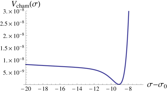
Figure 1: The chameleon potential as a function of $\sigma=R^{-2}$ with $A\equiv e^{-|a|\sigma_{0}}$. For clarity of visualisation we plot numerically reasonable values of the parameters instead of realistic ones.

The potential (2.7) has a local minimum, around which we can make a quadratic approximation for $R>R_{*}$, and at some $R<R_{*}$ we can approximate it by the leading exponential, $\sim e^{2|a|R^{-2}}$. However, because the minimum of the potential itself is made up from the same exponentials, we cannot treat the region around the minimum as independent from the region $R<R_{*}$.

The constraint for laboratory experiments was found [1, 14] to be expressed in terms of $R_{*}$ (here $R=R_{*}$ implies $\sigma=\sigma_{*}$),

$$\sigma_{*}=R_{*}^{-2}\mathrel{\mathstrut\smash{\ooalign{\raise 2.5pt\hbox{$>$}\cr\lower 2.5pt\hbox{$\sim$}}}}\frac{10^{30}}{|a|}\,,$$ (2.9)

which, together with accelerator constraints on $M_{10}$ and gravity constraints on $r$ can only by satisfied by $n=2$ large extra dimensions (in which case we have the $\sigma=R^{-2}$ as we have assumed until now). More precisely, we have now

$$M_{10} \mathrel{\mathstrut\smash{\ooalign{\raise 2.5pt\hbox{$<$}\cr\lower 2.5pt\hbox{$\sim$}}}} 2.5|a|^{1/2}~{}{\rm TeV}\,;$$ (2.12)

$$r_{*} \mathrel{\mathstrut\smash{\ooalign{\raise 2.5pt\hbox{$>$}\cr\lower 2.5pt\hbox{$\sim$}}}} \frac{100}{|a|}~{}\mu{\rm m}$$ (2.15)

We will consider in these constraints the natural value $|a|\sim 1$. To satisfy collider constraints (for $n\neq 2$, from the equivalent of (2.9) we would find either a $M_{10}$ too low such that it would have been observed at current accelerators, or $r_{*}$ too high so that gravity experiments would have seen this effect, and for $n=2$ (2.15) are only satisfied in a braneworld scenario; see [14] for more details), we then must have the Standard Model fields be confined to a brane, with the two large extra dimensions transverse to it, i.e. a $Dp$-brane with $p\leq 7$, situated at a fixed point in the extra dimensions.

The Kähler potential (2.6) implies that the canonical scalar field asssociated with $\varrho=i\sigma$ is

$$\phi=-M_{\rm Pl}\ln\frac{\sigma}{\sigma_{*}}\,,$$ (2.16)

where we have put $\phi=0$ at the present time, leading to a coupling function for the coupling to matter density (from (2.1))

$$A(\phi)\equiv\frac{R}{R_{*}}=e^{\phi/2M_{\rm Pl}}\,.$$ (2.17)

That means that the effective potential, including the coupling to matter density $\rho$ is

$$V_{\rm eff}(\phi)=V(\phi)+\rho\frac{R}{R_{*}}=V(\phi)+\rho e^{\phi/2M_{\rm Pl}}\,.$$ (2.18)

While a potential which can be approximated by a quadratic around the minimum up to $R=R_{*}$ was found in [1] to constrain the mass of the chameleon on cosmological scales as $m_{\rm cosmo}\mathrel{\mathstrut\smash{\ooalign{\raise 2.5pt\hbox{$>$}\cr\lower 2.5pt\hbox{$\sim$}}}}10^{3}H_{0}$, for the potential (2.7) we have $m_{\rm cosmo}\mathrel{\mathstrut\smash{\ooalign{\raise 2.5pt\hbox{$>$}\cr\lower 2.5pt\hbox{$\sim$}}}}10^{15}H_{0}$.

To avoid this stringent constraint, we now consider a racetrack type of superpotential [15], with two exponentials in the superpotential instead of one, i.e.

$$W(\varrho)=W_{0}+A_{1}e^{ia_{1}\varrho}+A_{2}e^{ia_{2}\varrho}\,,$$ (2.19)

with $a_{1},a_{2}<0$ and comparable, and $A_{1},A_{2}>0$ and comparable as well, leading to a potential

$$V(R) = \frac{1}{2M_{\rm Pl}^{2}}\left[\left(A_{1}a_{1}e^{|a_{1}|R^{-2}}+A_{2}a_{2}e^{|a_{2}|R^{-2}}\right)^{2}-2R^{2}\left(A_{1}|a_{1}|e^{|a_{1}|R^{-2}}+A_{2}a_{2}e^{|a_{2}|R^{-2}}\right)\times\right.$$ (2.21)

$$\left.\times\Big{(}W_{0}+A_{1}e^{|a_{1}|R^{-2}}\Big{)}-\frac{1}{2}R^{4}\Big{(}W_{0}+A_{1}e^{|a_{1}|R^{-2}}+A_{2}e^{|a_{2}|R^{-2}}\Big{)}^{2}\right]$$

We want the minimum and the leading exponential to be independent, so we need to choose the two exponentials to be very close, and $a_{1}$ to dominate the $\sigma>\sigma_{*}$ (or $R<R_{*}$) behaviour, while $a_{2}$ to dominate the minimum. In other words, we need $|a_{1}|>|a_{2}|$, yet very close in value, but we also need

$$A_{2}|a_{2}|e^{|a_{2}|\sigma_{\rm min}}>A_{1}|a_{1}|e^{|a_{1}|\sigma_{\rm min}}$$ (2.22)

The condition for the minimum is $D_{\varrho}W=\partial_{\varrho}W+(\partial_{\varrho}K)W=0$, which gives

$$A_{1}|a_{1}|\sigma_{\rm min}e^{|a_{1}|\sigma}+A_{2}|a_{2}|\sigma_{\rm min}e^{|a_{2}|\sigma}=W_{0}+A_{1}e^{|a_{1}|\sigma}+A_{2}e^{|a_{2}|\sigma}$$ (2.23)

which can be solved (with the above assumptions, and considering that $|a_{i}|\sigma_{\rm min}\gg 1$) by

$$\sigma_{\rm min}\simeq\frac{1}{|a_{1}|}\ln\frac{W_{0}}{|a_{1}|}$$ (2.24)

and for which the minimum is

$$V_{0}\simeq-\frac{3W_{0}^{2}}{4\sigma_{\rm min}^{2}M_{\rm Pl}^{2}}$$ (2.25)

By simply allowing for this kind of superpotential we are allowed more freedom to fix our parameters and thus find a successful embedding. However, we should be cautious of such tuning as such as was pointed out in [17] such potentials are not necessarily stable to all corrections. Our goal here is simply to prove in principle that such an embedding can be done.

3 Experimental constraints

We already mentioned the constraint (2.9) obtained from laboratory experiments. A weaker constraint appears from the fact that the Milky Way galaxy must be screened, otherwise the field value in the solar system, $\phi_{{\rm solar}\;{\rm system}}$, would not be fixed by the local density. That means that the galaxy needs to have a thin shell, i.e.

$$\left(\frac{3\Delta{\cal R}}{{\cal R}}\right)_{\rm galaxy}=\frac{\phi_{\rm cosmo}-\phi_{{\rm solar}\;{\rm system}}}{2gM_{\rm Pl}\Phi_{\rm G}}<1\,,$$ (3.1)

where $\Phi_{G}\sim 10^{-6}$ is the Newtonian potential of the galaxy and $g=1/2$ is the chameleon coupling (see (2.18)). Since the field variations are small, we have $|\Delta\sigma/\sigma|\simeq 2\Delta R/R=\Delta\phi/M_{\rm Pl}$, meaning we obtain the constraint

$$\frac{\sigma_{\rm min}-\sigma_{*}}{\sigma_{\rm min}}\simeq\frac{R_{\rm min}-R_{\rm solar\;system}}{2R_{*}}\;\mathrel{\mathstrut\smash{\ooalign{\raise 2.5pt\hbox{$<$}\cr\lower 2.5pt\hbox{$\sim$}}}}\;10^{-6}\,,$$ (3.2)

We will see later that this constraint is much weaker than (2.9), but constrains the same quantity.

We want to derive a constraint on the mass of the chameleon field on cosmological scales, when the chameleon is close to the minimum. Therefore we want to find the constraint on

$$m^{2}_{\rm cosmo}\simeq\frac{g^{2}R_{*}^{2}}{M_{\rm Pl}^{2}}\left.\frac{{\rm d}^{2}V}{{\rm d}R^{2}}\right|_{R=R_{\rm min}}=\frac{g^{2}R_{*}^{2}}{M_{\rm Pl}^{2}}\left[\frac{d\sigma}{dR}(R_{\rm min})\right]^{2}\frac{d^{2}V}{d\sigma^{2}}(\sigma_{\rm min})$$ (3.3)

Expanding the potential (2.21) around the minimum (2.24) with the value (2.25) for the potential, and assuming the condition (2.22), we find that

$$\frac{d^{2}V}{d\sigma^{2}}(\sigma_{\rm min})\simeq\frac{4}{3}a_{2}^{2}|V_{0}|$$ (3.4)

Substituting back in (3.3), and using $\sigma=R^{-2}$ and $g=1/2$, we get

$$m^{2}_{\rm cosmo}\simeq\frac{4}{3}a_{2}^{2}\sigma_{\rm min}^{2}\frac{|V_{0}|}{M_{\rm Pl}^{2}}$$ (3.5)

so we see that a constraint on $m_{\rm cosmo}$ comes from a constraint on $|V_{0}|$.

Such a constraint comes from imposing that the field value is not in the potential region of the leading exponential ($R<R_{*}$) in all the Universe, and that the low densities required to be on the quadratic region of the potential ($R>R_{*}$) are reached on some large scales, namely that the density $\rho_{*}$ corresponding to $R_{*}$ must be greater than the cosmic density,

$$\rho_{*}=R_{*}\left|\frac{{\rm d}V}{{\rm d}R}(R_{*})\right|\geq H_{0}^{2}M_{\rm Pl}^{2}\,.$$ (3.6)

But in the leading exponential region of the potential,

$$V(\sigma)-V_{0}\simeq\frac{A_{1}^{2}a_{1}^{2}}{2M_{\rm Pl}^{2}}e^{2|a_{1}|\sigma}$$ (3.7)

which gives

$$\rho_{*}=R_{*}\left|\frac{d\sigma}{dR}(R_{*})\frac{dV}{d\sigma}(\sigma_{*})\right|\simeq\frac{2|a_{1}|\sigma_{*}A_{1}^{2}a_{1}^{2}}{M_{\rm Pl}^{2}}e^{2|a_{1}|\sigma_{*}}\simeq\frac{8}{3}|a_{1}|\sigma_{\rm min}|V_{0}|e^{2|a_{2}|(\sigma_{*}-\sigma_{\rm min})}\geq H_{0}^{2}M_{\rm Pl}^{2}.$$ (3.8)

Since $a_{1}\simeq a_{2}$ and $\sigma_{\rm min}\simeq 10^{30}$, comparing (3.5) with (3.8), we see that now we have an extra factor, $e^{|a_{2}|(\sigma_{\rm min}-\sigma_{*})}$, to help. It was found in [1] that the constraint in the case of the phenomenological potential with an independent quadratic region near the minimum, and an unrelated leading exponential for $R<R_{*}$ was $m_{\rm cosmo}\geq 10^{3}H_{0}$. Since we could not do better, at most we can reach this constraint using the factor $e^{|a_{2}|(\sigma_{\rm min}-\sigma_{*})}$. Direct comparison shows that a factor of $e^{|a_{2}|(\sigma_{\rm min}-\sigma_{*})}=10^{12}$ would give us back the constraint $m_{\rm cosmo}\geq 10^{3}H_{0}$.

In the phenomenological potential, $\sigma_{*}$ (or $R_{*}$) is the separation point between the two (independent) parts of the potential, the quadratic and leading exponential. In the case of our potential, we need a definition compatible with this phenomenological one. Therefore we define $\sigma_{*}$ as the place where the derivative of the leading exponential equals the derivative of the other exponential, since this is indeeed the transition point from the leading exponential to the rest. We can check from (2.21) that this gives approximately

$$e^{(|a_{1}|-|a_{2}|)\sigma_{*}}=\frac{A_{2}a_{2}}{A_{1}a_{1}}$$ (3.9)

Calling by $K$ the ratio

$$K=\frac{A_{2}|a_{2}|e^{|a_{2}|\sigma_{\rm min}}}{A_{1}|a_{1}|e^{|a_{1}|\sigma_{\rm min}}}$$ (3.10)

which had to be bigger than 1 according to (2.22), the condition

$$e^{|a_{2}|(\sigma_{\rm min}-\sigma_{*})}=10^{12}$$ (3.11)

gives

$$\left(\frac{A_{2}|a_{2}|e^{|a_{2}|\sigma_{\rm min}}}{A_{1}|a_{1}|e^{|a_{1}|\sigma_{\rm min}}}=\right)K=10^{12\frac{(|a_{1}|-|a_{2}|)}{|a_{2}|}}$$ (3.12)

We now also note that we need

$$\sigma_{*}-\sigma_{\rm min}\simeq\frac{27}{|a_{2}|}$$ (3.13)

so going back to the galaxy screening constraint (3.2), it now translates into

$$|a_{2}|\sigma_{*}\mathrel{\mathstrut\smash{\ooalign{\raise 2.5pt\hbox{$>$}\cr\lower 2.5pt\hbox{$\sim$}}}}3\times 10^{7}$$ (3.14)

which is much weaker than (2.9).

From (3.8), with (3.11), we get

$$|V_{0}|\;\mathrel{\mathstrut\smash{\ooalign{\raise 2.5pt\hbox{$>$}\cr\lower 2.5pt\hbox{$\sim$}}}}\;\frac{10^{-144}}{|a_{1}|\sigma_{\rm min}}M_{\rm Pl}^{4}$$ (3.15)

The constraint on $|a_{1}|\sigma_{\rm min}$ goes the opposite way, but assuming it is saturated at $10^{30}$, we get

$$|V_{0}|\;\mathrel{\mathstrut\smash{\ooalign{\raise 2.5pt\hbox{$>$}\cr\lower 2.5pt\hbox{$\sim$}}}}\;10^{-174}M_{\rm Pl}^{4}$$ (3.16)

and then also (from (2.25))

$$W_{0}\;\mathrel{\mathstrut\smash{\ooalign{\raise 2.5pt\hbox{$>$}\cr\lower 2.5pt\hbox{$\sim$}}}}\;10^{-57}M_{\rm Pl}^{3}$$ (3.17)

The coefficients $A$ are again extremely small, but writing $A_{i}e^{|a_{i}|\sigma}=M_{\rm Pl}^{3}e^{|a_{i}|(\sigma-\sigma^{i}_{0})}$, we have $\sigma^{i}_{0}\sim-\log A_{i}/M_{\rm Pl}^{3}\sim 10^{30}$.

Finally, when adding the supersymmetry-breaking antibrane term $+D/\sigma^{2}$ to the potential, as in KKLT, we can fix the value of $\sigma$ as follows. For the $A$’s and $W_{0}$’s we took, the value of the supersymmetric potential today is close to $V_{\rm today}\sim-10^{-174}M_{\rm Pl}^{4}$, negligible compared to the observed positive cosmological constant, hence we can assume that all the cosmological constant term comes from the supersymmetry-breaking term, giving $D/\sigma_{*}^{2}\sim 10^{-122}M_{\rm Pl}^{4}$ or, since $\sigma_{*}\sim 10^{30}$, $D\sim 10^{-62}M_{\rm Pl}^{4}$.

4 Conclusions

In this paper we have considered a ”racetrack” type superpotential $W=W_{0}+A_{1}a^{ia_{1}\varrho}+A_{2}e^{ia_{2}\varrho}$ instead of the single KKLT exponential, in order to obtain a chameleon scalar from a string theory context, generalizing the work in [1]. We have also used the more natural large extra dimensional scenario from [14], in order to have $a_{1},a_{2}$ closer to what can be obtained in KKLT. The simple modification of the ”racetrack” allowed us to avoid having a too large chameleon mass on cosmological scales, and we found that we can have $m_{\rm cosmo}\geq 10^{3}H_{0}$, which can have implications interesting for cosmology.

Acknowledgements We would like to thank Kurt Hinterbichler, Justin Khoury and Rogerio Rosenfeld for discussions. The work of HN is supported in part by CNPQ grant 301219/2010-9. This material is based upon work supported financially by the National Research Foundation. Any opinion, findings and conclusions or recommendations expressed in this material are those of the authors and therefore the NRF does not accept any liability in regard thereto.

References

- [1] K. Hinterbichler, J. Khoury, and H. Nastase, “Towards a UV Completion for Chameleon Scalar Theories,” JHEP 1103 (2011) 061, arXiv:1012.4462 [hep-th].
- [2] ATLAS Collaboration Collaboration, G. Aad et al., “Observation of a new particle in the search for the Standard Model Higgs boson with the ATLAS detector at the LHC,” Phys.Lett. B716 (2012) 1–29, arXiv:1207.7214 [hep-ex].
- [3] CMS Collaboration Collaboration, S. Chatrchyan et al., “Observation of a new boson at a mass of 125 GeV with the CMS experiment at the LHC,” Phys.Lett. B716 (2012) 30–61, arXiv:1207.7235 [hep-ex].
- [4] J. Khoury and A. Weltman, “Chameleon Fields: Awaiting Surprises for Tests of Gravity in Space,” Phys. Rev. Lett. 93 (2004) 171104, arXiv:astro-ph/0309300.
- [5] J. Khoury and A. Weltman, “Chameleon Cosmology,” Phys. Rev. D69 (2004) 044026, arXiv:astro-ph/0309411.
- [6] P. Brax, C. van de Bruck, A.-C. Davis, J. Khoury, and A. Weltman, “Detecting dark energy in orbit - The Cosmological chameleon,” Phys.Rev. D70 (2004) 123518, arXiv:astro-ph/0408415 [astro-ph].
- [7] P. Brax, C. van de Bruck, A. Davis, J. Khoury, and A. Weltman, “Chameleon dark energy,” AIP Conf.Proc. 736 (2005) 105–110, arXiv:astro-ph/0410103 [astro-ph].
- [8] T. Damour and A. M. Polyakov, “The String dilaton and a least coupling principle,” Nucl.Phys. B423 (1994) 532–558, arXiv:hep-th/9401069 [hep-th].
- [9] T. Damour and A. M. Polyakov, “String theory and gravity,” Gen.Rel.Grav. 26 (1994) 1171–1176, arXiv:gr-qc/9411069 [gr-qc].
- [10] S. Kachru, R. Kallosh, A. D. Linde, and S. P. Trivedi, “De Sitter vacua in string theory,” Phys. Rev. D68 (2003) 046005, arXiv:hep-th/0301240.
- [11] H. Abe, T. Higaki, and T. Kobayashi, “KKLT type models with moduli-mixing superpotential,” Phys. Rev. D73 (2006) 046005, arXiv:hep-th/0511160.
- [12] F. Quevedo, “Lectures on superstring phenomenology,” arXiv:hep-th/9603074.
- [13] C. P. Burgess, A. de la Macorra, I. Maksymyk, and F. Quevedo, “Fixing the dilaton with asymptotically-expensive physics?,” Phys. Lett. B410 (1997) 181–187, arXiv:hep-th/9707062.
- [14] K. Hinterbichler, J. Khoury, H. Nastase, and R. Rosenfeld, “Chameleonic inflation,” arXiv:1301.6756 [hep-th].
- [15] F. Denef, M. R. Douglas, and B. Florea, “Building a better racetrack,” JHEP 0406 (2004) 034, arXiv:hep-th/0404257 [hep-th].
- [16] J. Blanco-Pillado, C. Burgess, J. M. Cline, C. Escoda, M. Gomez-Reino, et al., “Racetrack inflation,” JHEP 0411 (2004) 063, arXiv:hep-th/0406230 [hep-th].
- [17] B. Greene and A. Weltman, “An Effect of alpha’ corrections on racetrack inflation,” JHEP 0603 (2006) 035, arXiv:hep-th/0512135 [hep-th].
- [18] S. Kachru, J. Pearson, and H. L. Verlinde, “Brane / flux annihilation and the string dual of a nonsupersymmetric field theory,” JHEP 0206 (2002) 021, arXiv:hep-th/0112197 [hep-th].
- [19] P. Brax, C. Burrage, A.-C. Davis, D. Seery, and A. Weltman, “Anomalous coupling of scalars to gauge fields,” Phys.Lett. B699 (2011) 5–9, arXiv:1010.4536 [hep-th].
- [20] A. Upadhye, J. Steffen, and A. Weltman, “Constraining chameleon field theories using the GammeV afterglow experiments,” Phys.Rev. D81 (2010) 015013, arXiv:0911.3906 [hep-ph].
- [21] GammeV Collaboration Collaboration, J. H. Steffen et al., “Laboratory constraints on chameleon dark energy and power-law fields,” Phys.Rev.Lett. 105 (2010) 261803, arXiv:1010.0988 [astro-ph.CO].