Calling Patterns in Human Communication Dynamics

Abstract

Modern technologies not only provide a variety of communication modes, e.g., texting, cellphone conversation, and online instant messaging, but they also provide detailed electronic traces of these communications between individuals. These electronic traces indicate that the interactions occur in temporal bursts. Here, we study the inter-call durations of the 100,000 most-active cellphone users of a Chinese mobile phone operator. We confirm that the inter-call durations follow a power-law distribution with an exponential cutoff at the population level but find differences when focusing on individual users. We apply statistical tests at the individual level and find that the inter-call durations follow a power-law distribution for only 3460 individuals (3.46%). The inter-call durations for the majority (73.34%) follow a Weibull distribution. We quantify individual users using three measures: out-degree, percentage of outgoing calls, and communication diversity. We find that the cellphone users with a power-law duration distribution fall into three anomalous clusters: robot-based callers, telecom frauds, and telephone sales. This information is of interest to both academics and practitioners, mobile telecom operator in particular. In contrast, the individual users with a Weibull duration distribution form the fourth cluster of ordinary cellphone users. We also discover more information about the calling patterns of these four clusters, e.g., the probability that a user will call the $c_{r}$-th most contact and the probability distribution of burst sizes. Our findings may enable a more detailed analysis of the huge body of data contained in the logs of massive users.

Understanding the temporal patterns of individual human interactions is essential in managing information spreading and in tracking social contagion. Human interactions, e.g., cellphone conversations and emails, leave electronic traces that allow the tracking of human interactions from the perspective of either static complex networks Eckmann-Moses-Sergi-2004-PNAS ; Palla-Barabasi-Vicsek-2007-Nature ; Onnela-Saramaki-Hyvonen-Szabo-Menezes-Kaski-Barabasi-Kertesz-2007-NJP ; Onnela-Saramaki-Hyvonen-Szabo-Lazer-Kaski-Kertesz-Barabasi-2007-PNAS ; Jo-Pan-Kaski-2011-PLoS1 ; Kumpula-Onnela-Saramaki-Kaski-Kertesz-2007-PRL or human dynamics Barabasi-2005-Nature . Because static networks only describe sequences of instantaneous interacting links, temporal networks in which the temporal patterns of interacting activities for each node are recorded have recently received a considerable amount of research interest Holme-Saramaki-2012-PR ; Pan-Saramaki-2011-PRE . Investigations of inter-event intervals between two consecutive interacting actions, such as email communications Barabasi-2005-Nature ; Malmgren-Stouffer-Motter-Amaral-2008-PNAS , short-message correspondences Hong-Han-Zhou-Wang-2009-CPL ; Wu-Zhou-Xiao-Kurths-Schellnhuber-2010-PNAS ; Zhao-Xia-Shang-Zhou-2011-CPL , cellphone conservations Candia-Gonzalez-Wang-Schoenharl-Madey-Barabasi-2008-JPAMT ; Karsai-Kaski-Barabasi-Kertesz-2012-SR , and letter correspondences Oliveira-Barabasi-2005-Nature ; Li-Zhang-Zhou-2008-PA ; Malmgren-Stouffer-Campanharo-Amaral-2009-Science , indicate that human interactions have non-Poissonian characteristics. Previous studies were conducted either on aggregate samples Candia-Gonzalez-Wang-Schoenharl-Madey-Barabasi-2008-JPAMT ; Karsai-Kaski-Barabasi-Kertesz-2012-SR ; Karsai-Kaski-Kertesz-2012-PLoS1 or on a small group of selected individuals Barabasi-2005-Nature ; Oliveira-Barabasi-2005-Nature ; Li-Zhang-Zhou-2008-PA ; Malmgren-Stouffer-Motter-Amaral-2008-PNAS ; Malmgren-Stouffer-Campanharo-Amaral-2009-Science ; Hong-Han-Zhou-Wang-2009-CPL ; Wu-Zhou-Xiao-Kurths-Schellnhuber-2010-PNAS , but the communication behavior of individuals is not well understood.

We study the complete voice information for cellphone users supplied by a Chinese cellphone operator and study the inter-event time between two consecutive outgoing calls (inter-call duration). Our studies are performed at both the individual and group levels. To ensure better statistics, the top 100,000 cellphone users with the largest number of outgoing calls are chosen as our data sample, each having more than 997 outgoing calls. We propose a bottom-up approach to investigate individual cellphone communication dynamics: (1) finding the functional form of the distribution of each individual’s intercall durations, (2) grouping individuals with the same distribution, and (3) understanding the calling patterns for each group. We apply an automatic fitting technology to each mobile phone user, and filter out two groups of users according to their inter-call duration distributions. One group is comprised of individuals with a power-law duration distribution (3,464 individuals) and the other is comprised of individuals with a Weibull duration distribution (73,339 individuals). We demonstrate that the two groups exhibit different calling patterns and that the individuals from the power-law group exhibit anomalous communication behaviors (e.g., the group includes individuals sending spam).

Results

Distribution at the population level. There are 5,921,696 different individuals in our data set (see the data description in Materials and Methods). For each individual, we estimate the intraday inter-call durations ($d$ seconds) (see definition of intraday inter-call durations in Materials and Methods) and we find that 4,635,536 individuals have non-empty intraday durations ($n_{d}>0$), which we consider one unique sample when we investigate the distribution at the population level. To this end we also analyze the aggregate level where the data comprise only the durations of the top 100,000 individuals.

Figure 1A shows the empirical distributions of the two samples of aggregate data. Both curves exhibit excellent power law behaviors in the range of [80,2000] seconds. We apply the least-square method, and find that a linear fit gives the power-law exponent $\gamma_{\rm{all}}=0.873$ for all the individuals and $\gamma_{{\rm{top}}~{}10^{5}}=0.942$ for the top 100,000 individuals, respectively. We compare the empirical distributions obtained from our dataset with the empirical distributions of inter-call durations based on a different dataset provided by a European cellphone operator Candia-Gonzalez-Wang-Schoenharl-Madey-Barabasi-2008-JPAMT (see also the supplementary information of Ref. Gonzalez-Hidalgo-Barabasi-2008-Nature ), and note that the empirical distributions of both datasets share very similar patterns for $d\leq 10^{5}$, where only intraday inter-call durations are taken into consideration. The reported power-law exponent $\gamma=0.9$ in Ref. Gonzalez-Hidalgo-Barabasi-2008-Nature is approximately equal to the estimated exponents $\gamma_{\rm{all}}$ shown in Fig. 1A. A similar functional form with a power-law exponent $\gamma=0.7$ is also reported in Ref. Karsai-Kaski-Barabasi-Kertesz-2012-SR for inter-call durations smaller than $10^{5}$. This similarity is further consolidated by fitting the empirical duration distributions by means of a formula of power-law with an exponential cutoff.

Figure 1: Probability distribution of the inter-call durations ($d$ seconds). (A) Distribution of inter-call durations at the population level. The circle markers are shifted vertically by a factor of 0.1 for better visibility. (B) Plots of the statistic $\rm{KS}$ with respect to the truncated value $d_{\rm{trun}}$ for Weibull and exponential distribution. (C) Plots of the power-law exponent $\gamma$ with respect to the average number of outgoing calls $\langle n_{\rm{call}}\rangle$ for different groups. The red line stands for the power-law exponent of the whole sample. (D) Probability distribution of mean inter-call durations for different samples of individuals.

Figure 1A shows a clear deviation from the power-law distribution in the tails of both curves, which is usually interpreted as an exponential cut-off. To test which distribution better fits the data, we apply Kolmogorov-Smirnov (KS) statistics by means of which the smaller the value, the better the fit. We set the truncation value at 2000 seconds and find that for all individuals the tail is better fit by the Weibull distribution ($\rm{KS}=0.016$) than by the exponential distribution ($\rm{KS}=0.063$). Similarly, for the top $10^{5}$ individuals the Weibull distribution ($\rm{KS}=0.006$) also fits the data better than the exponential distribution ($\rm{KS}=0.066$). Figure 1B for varying truncation values shows a plot of $\rm{KS}$ as a function of $d_{\rm{trun}}$. The $\rm{KS}$ statistic displays a more stable behavior for the Weibull fit than for the exponential fit, indicating that the Weibull distribution is better able to capture the tail behavior than the exponential distribution.

We further divide the sequence of individuals according to the number of outgoing calls into 46 groups, sorted in ascending order. The first group comprises 135,536 individuals and the remaining 45 groups each comprise 100,000 individuals. We calculate the empirical distributions of the aggregate inter-call durations for each group and find that all the distributions share patterns similar to those shown in Fig. 1A. Figure 1C shows a plot of the estimated power-law exponents with respect to the average number of outgoing calls. All the power-law exponents are lower than 1 and the mean value is $0.896\pm 0.033$.

Figure 1D shows the probability distributions of the individual average inter-call durations calculated for (i) all the individuals, (ii) the individuals with $n_{d}\geq 50$, and (iii) the top 100,000 individuals, respectively. All three curves exhibit an approximate $M$-shape characterized by two peaks. For the sample of all individuals, there is a large number of low-frequency individuals who do not use a cellphone regularly. The influence of these low-frequency callers is eliminated in the distributional curve of $n_{d}\geq 50$. We compare this distributional curve with the distribution of the top 100,000 individuals and find that they exhibit the same $M$-shape with a central valley at approximately $d=650$, strongly indicating the presence of two groups of individuals possessing different calling patterns across the sample. One group is of individuals that have low average inter-call duration values, indicating a high frequency of outgoing calls, and the other is of individuals that have large average inter-call duration values, indicating a relatively low frequency of outgoing calls. We will later demonstrate that the group with a high frequency of outgoing calls is dominated by individuals with a power-law duration distribution and that the group with a low frequency of outgoing calls is dominated by the individuals with a Weibull duration distribution.

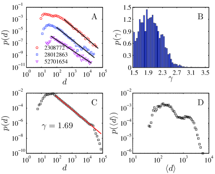
Figure 2: Classified results of individuals with power-law distributions of intraday inter-call durations. (A) Probability distributions of intraday durations for three randomly chosen individuals. The markers of individual 28012863 and 52701654 are shifted vertically by a factor of $10^{-2}$ and $10^{-4}$ for better visibility. The solid lines are the best maximum likelihood estimation (MLE) fit to the power-law distributions, which gives the power-law exponents $\gamma=2.15$, $\gamma=2.03$, and $\gamma=1.69$ for individual 2308772, 28012863, and 52701654, respectively. (B) Distribution of the estimated power-law exponents. (C) Probability distribution of collective inter-call durations by aggregating the durations of different individuals from the power-law group as one sample. The solid line is the best fit to the data by means of the least-square method, which gives an estimation of power-law exponent $\gamma=1.69$. (D) Probability distribution of the mean inter-call durations for the power-law group.

Classification of cellphone users. According to the above analysis at the aggregate level, we propose to classify the individuals according to their duration distributions. Motivated by Ref. Clauset-Shalizi-Newman-2009-SIAMR , but here for each individual cellphone user, because we are focusing on the tail of the distribution we assume the candidate duration distributions to be left-truncated and we assign each of them a distribution that is either power law or Weibull. We estimate the truncation value $d_{\min}$ associated with distribution parameters by finding the minimum KS statistic. We then apply statistical tests to check the significance of the fitting parameters (see fitting distributions and statistical tests in Materials and Methods). Finally, based on statistical tests, we find that there are 3,464 individuals whose intraday durations follow a power-law distribution and 73,339 individuals whose intraday durations follow a Weibull distribution (see determining the distribution form in Materials and Methods).

Figure 2A shows that the empirical duration distributions for three randomly chosen individuals (2308772, 28012863, and 52701654) whose intraday inter-call durations follow a power-law distribution. The solid lines correspond to the power-law fits with power-law exponents $\gamma=2.15$, $\gamma=2.03$, and $\gamma=1.69$ for individuals 2308772, 28012863, and 52701654, respectively. Figure 2B plots the distribution of the estimated power-law exponents $\gamma$ for all individuals with an intraday inter-call duration that follows a power-law distribution and finds that none of the power-law exponents are lower than 1.5. This is in sharp contrast to the power-law exponents lower than 1 that we found for the aggregate durations in Fig. 1C. Note that there is a large fraction of individuals whose power-law exponents are between 1 and 3, which are the characteristic values for the Lévy regime $(1,3)$. Note that the exponent 2 corresponds to the famous Zipf law. Having all the power-law exponents, we calculate the mean $\langle\gamma\rangle=2.00\pm 0.32$.

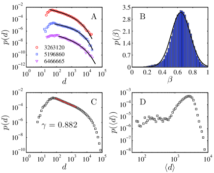
Figure 3: Classified results of individuals with Weibull distributions of intraday inter-call durations. (A) Probability distributions of intraday durations for three randomly chosen individuals. The markers of individual 5196860 and 6466665 are shifted vertically by a factor of $10^{-2}$ and $10^{-4}$ for better visibility. The solid lines are the best MLE fit to the Weibull distributions, which give the Weibull exponents $\beta=0.54$, $\beta=0.64$, and $\beta=0.51$ for individual 3263120, 28012863, and 6466665, respectively. (B) Distribution of the Weibull exponents and the solid curve stands for the fits to normal distribution. (C) Probability distribution of collective inter-call durations by aggregating the durations of different individuals from the Weibull group as one sample. The solid line is the best fit to the data by means of the least-square method, which gives an estimation of power-law exponent $\gamma=0.882$. (D) Probability distribution of the mean inter-call durations for the Weibull group.

We investigate the distribution of the aggregate intraday inter-call durations by treating the individual durations from the power-law group as one unique sample. To this end, for the aggregate data set in Fig. 2C, we find a power law with exponent $\gamma=1.69$. We find another striking feature in the power-law tail: the Weibull shape disappears. Figure 2D plots the probability distribution of the mean of inter-call durations of the individuals in the power-law group, where the peak agrees well with the left peak in Fig. 1D.

Figure 3 plots the probability distribution of intra-call durations for three randomly chosen individuals (3263120, 28012863, and 6466665) whose inter-call durations follow a Weibull distribution. The solid lines are the best maximum likelihood estimation (MLE) fits to the Weibull distribution and the corresponding Weibull exponents are $\beta=0.54$, $\beta=0.64$, and $\beta=0.51$ for individuals 3263120, 28012863, and 6466665, respectively. Having the Weibull exponents for all individuals from the Weibull group, we calculate the mean value of the Weibull exponents $\langle\beta\rangle=0.64\pm 0.12$. Figure 3B shows the distribution of the Weibull exponents $\beta$. For sake of comparison, we also present a normal distribution with the parameters obtained by MLE fits on the sample of Weibull exponents $\beta$. The overlapping between the empirical data and the normal distribution indicates that the exponent $\beta$ follows the normal distribution.

Figure 3C shows the distribution of inter-call durations for the Weibull group at the aggregate level. Note that the functional forms of the distribution in Fig. 3C and the empirical distributions in Fig. 1A are similar, suggesting that the distributions of the aggregate samples are dominated by individuals with Weibull duration distributions. Figure 3D plots the probability distribution of the mean inter-call durations for the individuals in the Weibull group. The peak is in good agreement with the right peak in Fig. 1D.

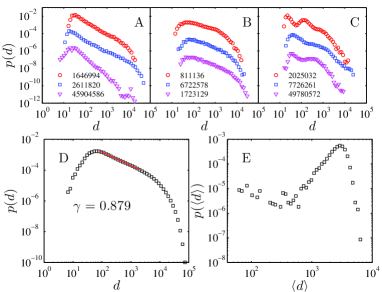
Figure 4: Analysis of the remaining individuals. (A) Probability distribution of inter-call durations for three individuals, whose durations approach to power-law behaviors without passing the statistical tests. (B) Probability distribution of inter-call durations for three individuals, whose duration distributions are like Weibull shape but not confirmed by the statistical tests. (C) Plots of duration distributions for three individuals, whose distribution shapes are uncommon. (D) Probability distribution of collective inter-call durations by aggregating the durations of different individuals from the Weibull group as one sample. The solid line is the best fit to the data by means of the least-square method, which gives an estimation of power-law exponent $\gamma=0.879$. (E) Probability distribution of the mean inter-call durations for the remaining individuals.

We next investigate the distribution of inter-call durations for the remaining 23,197 individuals. We find that for a small fraction of individuals (close to 2%), the inter-call durations follow a power law, as shown in Fig. 4A. Because our statistical tests reject the null hypothesis that individuals follow approximately a power law, these individuals are excluded from the power-law group. We find that more than 97% of the individuals have Weibull tail distributions, as shown in Fig. 4B. However the fact that the fitting range is lower than 1.5 orders of magnitude (83% of the individuals are in the range of $[1,1.5]$) disallows these individuals from being classified in the Weibull group. Figure 4C shows a very small number of individuals whose inter-call durations cannot be described by either power law or Weibull distributions. Because most of the individuals have Weibull-tail distributions, the distributions of aggregate inter-call durations and the mean inter-call durations exhibit patterns very similar to the results obtained from the Weibull group [see Figs. 4D and 4E and Figs. 3C and 3D].

Calling patterns for power-law and Weibull groups. Using three measurements, we quantitatively distinguish the calling patterns of the individuals belonging to two different classified groups.

• The out-degree $k_{i}$ describes the number of different callees for a specified cellphone user.

• The percentage of outgoing calls $r_{\rm{out}}$, is defined by dividing the number of outgoing calls by the total number of calls—note that the number sending spams (junk message pusher) is characterized by $r_{\rm{out}}=1$.

• The communication diversity $\phi$. Motivated by the social diversity proposed in Ref. Eagle-Macy-Claxton-2010-Science , we define the communication diversity $\phi_{i}$, as a function of Shannon entropy to quantify how the cellphone users split the number of calls to their friends,

  $$\phi_{i}=\frac{-\sum_{j=1}^{k_{i}}p_{ij}\log(p_{ij})}{\log(k_{i})}.$$ (1)

  Here $k_{i}$ is the out-degree and $p_{ij}$ is the probability defined as $p_{ij}=n_{I}^{ij}/n_{I}^{i}=n_{I}^{ij}/\sum_{j}^{k}n_{I}^{ij}$, where $n_{I}^{ij}$ is the number of outgoing calls from individual $i$ to individual $j$ and $n_{I}^{i}$ is the total number of outgoing calls for individual $i$. A higher $\phi_{i}$ value indicates that the caller’s outgoing calls are split more evenly to his friends and a smaller $\phi_{i}$ value implies that most of the caller’s outgoing calls are to only one of his friends. Note that we define $\phi_{i}=0$ when $k_{i}=1$.

In order to distinguish between the calling patterns of the power-law group of Fig. 2 and the Weibull group of Fig. 3, in Fig. 5 we plot the distribution of the percentage of outgoing calls $r_{\rm{out}}$ and the distribution of the communication diversity $\phi$. Figures 5A and 5C compare strikingly different patterns: (i) in the power-law group, the probability $p(r_{\rm{out}})$ is a monotonically increasing function of $r_{\rm{out}}$ that reaches a maximum value at $r_{\rm{out}}=1$ (the characteristic value for spam), but in the Weibull group, the frequency $p(r_{\rm{out}})$ is a non-monotonic function of $r_{\rm{out}}$ that has its maximum value close to the center at $r_{\rm{out}}=0.56$, and (ii) in the power-law group, the probability $p(\phi)$ exhibits three pronounced peaks at $\phi=0$, $\phi=0.84$, and $\phi=1$, but in the Weibull group, the probability $p(\phi)$ has only one peak at $\phi=0.82$. We further estimate the average value of the percentage of outgoing calls $\langle r_{\rm{out}}\rangle=0.89\pm 0.13$ for the power-law group and $\langle r_{\rm{out}}\rangle=0.57\pm 0.11$ for the Weibull group. Our analysis indicates that the individuals in the power-law group exhibit more extreme calling behaviors than those in the Weibull group, e.g., highly-frequent call initiation, a high percentage of outgoing calls, and either all calls to only one callee or equally distributing calls among all callees.

Figures 5B and 5D plot the out-degree $k$ with respect to the communication diversity $\phi$ and thus provide additional evidence that the behavior of individuals in the power-law group differs greatly from the behavior of individuals in the Weibull group. The individuals in the power-law group form three clusters in the $(\phi,k)$ plane, which are highlighted by the three ellipses in panel (B). The three clusters are also consistent with the three peaks of $f(\phi)$ in Fig. 5A. Figure 5D, on the other hand, shows only one large cluster for the Weibull group. Taking the two panels together, we see that the communication diversity $\phi$ increases with the out-degree $k$ on average. In the power-law group we further assign the individuals with $\phi\leq 0.1$ to cluster 1, the individuals with $0.7\leq\phi\leq 0.9$ and $50\leq k\leq 200$ to cluster 2, and the individuals with $\phi\geq 0.9$ and $k\geq 700$ to cluster 3. We find that there are 762, 710, and 1369 individuals, respectively, with average degrees of 21.76, 114.98, and 2083.3, respectively, in which the mean percentage of outgoing calls is 0.99, 0.80, and 0.94 in clusters 1, 2, and 3, respectively. We assign the individuals in the Weibull group to cluster 4 and find that the average degree and mean percentage of outgoing calls are 245.13 and 0.57, respectively. From our analysis, we first infer that the individuals in power-law cluster 1—the ones characterized by a high frequency of call initiation, a small number of callees, or an allocation of almost all outgoing calls to only one callee—are robot-based users. We next see that the individuals in cluster 3—the ones characterized by high frequency of call initiation, a large number of callees, and an even distribution of outgoing calls among all callees—are associated with telecom frauds and telephone sales. We also note that the individuals in cluster 4 are ordinary cellphone users. We next describe further differences in cellphone communication activities among the 4 clusters, e.g., the probability that a caller will call the $c_{r}$-th most contact and the burst size probability during burst periods.

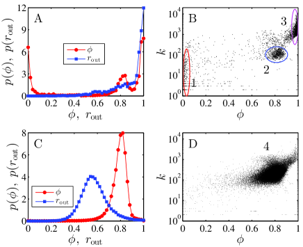
Figure 5: Calling patterns for the individuals from power-law and Weibull group. (A) Distribution of the percentage of outgoing calls $r_{\rm{out}}$ and the call diversity $\phi$ for power law group. (B) Plots of out-degree $k$ with respect to communication diversity $\phi$ for power law group. Three ellipses correspond to the three clusters of individuals. (C) Similar as (A) but for Weibull group. (D) Similar as (B) but for Weibull group.

Because most of the calls (mean 99.5% and min 94%) made by individuals in cluster 1 are to only one contact, we now calculate the probability that individuals belonging to the other 3 clusters will only call the $c_{r}$-th most contact. In order to rule out the influence of newly entering cellphone users, we take into account only those individuals listed in the data on the starting date of 28 June 2012. Figure 6 shows the average calling frequency $f(c_{r})$ of the $c_{r}$-th most contact friends for the individuals with the same degree in cluster 2. There is a linear relationship between $f(c_{r})$ and $\ln c_{r}$ in panel A, which indicates an exponential distribution in the number of outgoing calls to different contacts Sornette-2000 . We see that the slope obtained between $f(c_{r})$ and $\ln c_{r}$ increases as the out-degree $k$ increases, but the lack of individuals prevents us from finding the functional form between the slopes and the out-degree values $k$. We also observe power-law behavior between $f(c_{r})$ and $c_{r}$ in cluster 3 of panel (B). The least-square linear fits provide an estimate for power-law exponent $0.52$ and also show that the behavior of the power-law exponent is not affected by the out-degree $k$. Figure 6C plots $f(c_{r})^{b}$ versus $\ln c_{r}$ for cluster 4, where $b$ is associated with the maximum correlation coefficient of least-square linear fits to $f(c_{r})^{b}$ versus $\ln c_{r}$ by varying $b$ from 0.01 to 0.99 with a step of 0.01. The linear relationship between $f(c_{r})^{b}$ and $\ln c_{r}$ suggests that the number of outgoing calls to contacts follows a stretched exponential distribution Sornette-2000 ; Laherrere-Sornette-1998-EPJB . In panel (D) we show the exponent $b$ plotted with respect to the out-degree $k$, where we observe a striking linear relationship: $b=-4.836\times 10^{-4}k+0.329$. Here we report that the probability to call the $c_{r}$-th most contact is in sharp contrast to the results reported in Ref. Bagrow-Lin-2012-PLoS1 , where a Zipf law with a power-law exponent 1.5 is observed when, in contrast to our “microscopic” study, individuals are not grouped according to their distributions of inter-call durations.

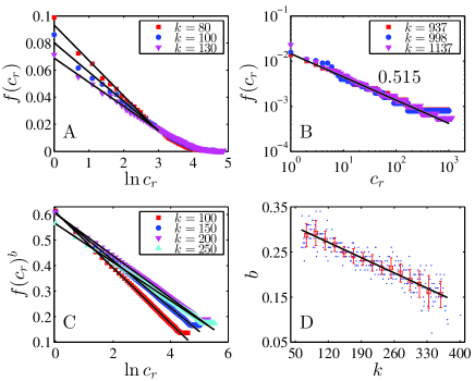
Figure 6: Rank ordering plot showing the average calling frequency $f(c_{r})$ of the $c_{r}$-th most contacted friend for the users with the same degree. (A) Plots of $f(c_{r})$ as a function of $\ln c_{r}$ for cluster 2. (B) Loglog plots of $f(c_{r})$ with respect to $c_{r}$ for cluster 3. (C) Plots of $f(c_{r})^{b}$ versus $\ln c_{r}$ for cluster 4. (D) Scatter plots of $b$ with respect to $k$ for cluster 4.

It was recently proposed that the distribution of burst sizes indicates the presence of memory behaviors in the timing of consecutive events Karsai-Kaski-Barabasi-Kertesz-2012-SR , where the deviation from exponential distributions is a hallmark of correlated properties. For a given series of events, a burst period is a cluster of consecutive events following their previous events within a short time interval $\Delta t$, which is an arbitrarily assigned value in empirical analysis. The burst size $e_{b}$ is defined as the number of events in a burst period.

Based on our dataset, Fig. 7 shows the probability distribution of burst sizes $e_{b}$ in burst periods at the aggregate level for the 4 clusters by setting $\Delta t$ = 100, 300, 600, and 1000 seconds. In panel A we find the probability distributions of $e_{b}$ for cluster 1. Although we find a very good power-law relationship between $p(e_{b})$ and $e_{b}$ with an exponent 2.677 for $\Delta t=100$ seconds, the distributions deviate from power-law distributions and tend to exponential distributions for $\Delta t$ = 300, 600, and 1000 seconds. Panel (B) shows that the probability distribution of $e_{b}$ exhibits excellent exponential distributions for varying values of $\Delta t$ for cluster 2. Panel (C) plots the probability distributions of $e_{b}$ for cluster 3. We see the power-law behavior of $p(e_{b})$ with an exponent 2.61 only when $\Delta t=300$ seconds. When $\Delta t$ = 600 and 1000 seconds, $p(e_{b})$ switches from power-law behavior to a bimodal pattern (with exponential tails). Panel (D) shows that the probability distributions of $e_{b}$ corresponding to different values of $\Delta t$ for individuals in cluster 4 all display very good power-law behavior, and that the power-law decay exponent is 3.6. Comparing our distribution with the distribution reported in Fig. 2A in Ref. Karsai-Kaski-Barabasi-Kertesz-2012-SR , we find that the distribution shapes are very similar for cluster 4, the only difference being that the extremely large brust sizes $e_{b}\geq 500$ disappear in the plots for the individuals with very long burst sizes assigned into cluster 1.

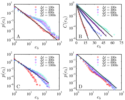
Figure 7: Distribution of burst sizes $e_{b}$ in burst periods. (A) Cluster 1 (PDF). (B) Cluster 2 (CDF). (C) Cluster 3 (PDF). (D) Cluster 4 (PDF).

Discussion

Contrary to common belief, we find that only 3.46% of callers have inter-call durations that follow a power-law distribution. The majority of callers (73.34%) have inter-call durations that follow a Weibull distribution. Further examination reveals that callers with a power-law distribution exhibit anomalous and extreme calling patterns often linked to robot-based calls, telecom frauds, or telephone sales—information valuable to both academics and practitioners, especially mobile telecom providers. We note that Weibull distributions are ubiquitous in such routine human activities as intervals for online gamers Jiang-Zhou-Tan-2009-EPL and intertrade intervals in stock trading Ivanov-Yuen-Podobnik-Lee-2004-PRE ; Jiang-Chen-Zhou-2008-PA .

Although most of the individuals exhibit Weibull distributions of the inter-call durations, the distribution at the population level is a power law with an exponential cutoff, consistent with other works using mobile phone communication data from other sources Gonzalez-Hidalgo-Barabasi-2008-Nature ; Karsai-Kaski-Barabasi-Kertesz-2012-SR . We argue that a superposition of individuals’ heterogeneous calling behaviors leads to the exponentially truncated power-law distribution at the population level, showing the importance of different characteristic scales.

Although individual callers exhibit heterogeneities across the entire population and their personal activities are also heterogeneous, individual callers can be grouped into clusters according to their similarities. The findings reported in this paper enable us to construct dynamic models at an individual level that agree with empirical collective properties. Every reasonable dynamic model for cellphone usage should include the major findings of this paper, i.e., that individuals are not identical and do not exhibit identical behavior. Our strategy is to propose models based, not on individuals, but on clusters of individuals. Thus to accurately model the trigger process in human activity we need a precise classification of individuals according to the similarities in their activities, and also a detailed investigation of the complete activity log for each individual.

Materials and Methods

Data description. Our data, which are provided by a cellphone provider in China, contain all the calling records covering two periods. One is from 28 June 2010 to 24 July 2010 and the other is from 1 October 2010 to 31 December 2010. For unknown reasons, the calling logs for a few hours on certain days (Ocotober 12, November 5, 6, 13, 21, and 27 and December 6, 8, 21, and 22) are missing, and they are excluded from our analysis, which results in a total of 109 days.

For each entry of record, we have the information of caller number, callee number, call starting time, call length, and call status. The caller and callee number is encrypted in order to protect personal privacy. The call status indicates whether the call is terminated normally. Note that we only take into account normal calls that the call begins and ends normally. The calls that are not completed or are interrupted, are also discarded. To better explain our data, Fig. 8 A shows the call records for a given individual subscriber, where a call starts at $t^{s}$ and ends at $t^{e}$. We usually have

$$\cdots<t_{i}^{s}<t_{i}^{e}<t_{i+1}^{s}<t_{i+1}^{e}<\cdots.$$ (2)

Further examination is made to check whether $t_{i}^{e}$ is less than $t_{i+1}^{s}$ for each individual. The records that do not obey the equation $t_{i}^{e}<t_{i+1}^{s}$ can be attributed to the recording errors introduced by the system and the $i+1$-th call record is discarded.

Definition of intraday inter-call durations. As shown in Fig. 8 A, the inter-call duration is defined as the time that elapses between two consecutive calls and it can be calculated via $d_{i}=t^{s}_{i}-t^{s}_{i-1}$. In order to avoid the influence on the results of discontinuous recording days, which produce very large inter-call durations, we restrict the durations to a period of one day (the typical human circadian rhythm). Although it might seem obvious to separate the days at midnight (00:00 AM), late night calls (made by lonely people, lovers, and friends) are common, so we divide the days at 4:00 A.M., which is the time point associating with the lowest call volume in a 24-hour period [see Fig. 8B]. This allows us to take into account the people who go out and stay awake later as well. Our restriction is equivalent to excluding inter-call durations that span the dividing point (4:00 AM).

Fitting distributions and statistical tests. A simple approach based on maximum likelihood estimation (MLE) fits and Kolmogorov-Smirnov (KS) tests is used to check whether the candidate distributions (power-law or Weibull) can be used to fit the individual intraday inter-call durations. Because people are more interested in the distribution form of large durations, we assume that the durations larger than a truncated value $d_{\min}$ are described by the candidate distributions, such that

$$p(d) \sim d^{-\gamma},~{}~{}d\geq d_{\min}$$ (3)

$$p(d) = \alpha\beta d^{\beta-1}\exp(-\alpha d^{\beta}),~{}~{}d\geq d_{\min}.$$ (4)

We also determine the lowest boundary $d_{\min}$ as an additional parameter. Once $d_{\min}$ is obtained, the distribution parameters can be estimated by means of MLE fits to the left-truncated candidate distribution. Hence, the accuracy of estimated $d_{\min}$ plays an important role in estimating accurate distribution parameters. Inspired by the method proposed in Ref. Clauset-Shalizi-Newman-2009-SIAMR , the best $d_{\min}$ is associated with the truncated sample with the smallest KS value. The truncated sample is obtained by discarding the durations below $d_{\min}$ in the original duration sample. After the lowest $d_{\min}$ and the corresponding distribution parameters are obtained, we use the KS test and CvM test to check the fitting. The null hypothesis $H_{0}$ for our KS test and CvM test is that the data ($d>d_{\min}$) are drawn from the candidate distribution (power-law distribution or Weibull distribution).

Determining the distribution form. The sample of individual intraday inter-call durations, which we assume conforms to a power-law distribution, must (i) pass either of the two tests at the significant level 0.01 and (ii) exhibit a fitting range of not less than 1.5 orders of magnitude. For Weibull distributions, in addition to the two above conditions, the Weibull exponent $\beta$ of the intraday duration sample must be in the range $(0,1)$. Because a power-law distribution is a two-parameter model and a Weibull distribution is a three-parameter model, we first filter out the individuals with durations that follow a power-law distribution and than inject the remaining individuals into the Weibull filtering procedure.

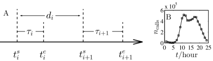
Figure 8: Definition of intraday inter-call durations. (A) Schematic chart of call logs for an individual. (B) Intraday pattern of the number of calls.

Acknowledgments:

Z.-Q.J., W.-J.X., M.-X.L. and W.-X.Z received support from the National Natural Science Foundation of China Grant 11205057, the Humanities and Social Sciences Fund (Ministry of Education of China Grant 09YJCZH040), and the Fok Ying Tong Education Foundation Grant 132013. BP and HES received support from the Defense Threat Reduction Agency (DTRA), the Office of Naval Research (ONR), and the National Science Foundation (NSF) Grant CMMI 1125290.

References

- (1) Eckmann JP, Moses E, Sergi D (2004) Entropy of dialogues creates coherent structures in e-mail traffic. Proc Natl Acad Sci USA 101:14333–14337.
- (2) Palla G, Barabási AL, Vicsek T (2007) Quantifying social group evolution. Nature 446:664–667.
- (3) Onnela JP, et al. (2009) Analysis of a large-scale weighted network of one-to-one human communication. New J Phys 9:179.
- (4) Onnela JP, et al. (2007) Structure and tie strengths in mobile communication networks. Proc Natl Acad Sci USA 104:7332–7336.
- (5) Jo HH, Pan RK, Kaski K (2011) Emergence of bursts and communities in evolving weighted networks. PLoS One 6:e22687.
- (6) Kumpula JM, Onnela JP, Saramäki J, Kaski K, Kertész J (2007) Emergence of communities in weighted networks. Phys Rev Lett 99:228701.
- (7) Barabási AL (2005) The origin of bursts and heavy tails in human dynamics. Nature 435:207–211.
- (8) Holme P, Saramäki J (2012) Temporal networks. Phys Rep 519:97–125.
- (9) Pan RK, Saramäki J (2011) Path lengths, correlations, and centrality in temporal networks. Phys Rev E 84:016105.
- (10) Malmgren RD, Stouffer DB, Motter AE, Amaral LAN (2008) A Poissonian explanation for heavy tails in e-mail communication. Proc Natl Acad Sci USA 105:18153–18158.
- (11) Hong W, Han XP, Zhou T, Wang BH (2009) Heavy-tailed statistics in short-message communication. Chin Phys Lett 26:028902.
- (12) Wu Y, Zhou CS, Xiao JH, Kurths J, Schellnhuber HJ (2010) Evidence for a bimodal distribution in human communication. Proc Natl Acad Sci USA 107:18803–18808.
- (13) Zhao ZD, Xia H, Shang MS, Zhou T (2011) Empirical analysis on the human dynamics of a large-scale short message communication system. Chin Phys Lett 28:068901.
- (14) Candia J, et al. (2008) Uncovering individual and collective human dynamics from mobile phone records. J Phys A: Math Theor 41:224015.
- (15) Karsai M, Kaski K, Barabási AL, Kertész J (2012) Universal features of correlated bursty behaviour. Sci Rep 2:397.
- (16) Oliveira JG, Barabási AL (2005) Darwin and Einstein correspondence patterns. Nature 437:1251.
- (17) Li NN, Zhang N, Zhou T (2008) Empirical analysis on temporal statistics of human correspondence patterns. Physica A 387:6391–6394.
- (18) Malmgren RD, Stouffer DB, Campanharo ASLO, Amaral LAN (2009) On Universality in Human Correspondence Activity. Science 325:1696–1700.
- (19) Karsai M, Kaski K, Kertétz J (2012) Correlated dynamics in egocentric communication networks. PLoS One 7:e40612.
- (20) González MC, Hidalgo CA, Barabási AL (2008) Understanding individual human mobility patterns. Nature 453:779–782.
- (21) Clauset A, Shalizi CR, Newman MEJ (2009) Power-law distributions in empirical data. SIAM Rev 51:661–703.
- (22) Eagle N, Macy M, Claxton R (2010) Network diversity and economic development. Science 328:1029–1031.
- (23) Sornette D (2000) Critical Phenomena in Natural Sciences - Chaos, Fractals, Self-organization and Disorder: Concepts and Tools (Springer, Berlin), 1 edn.
- (24) Laherrère J, Sornette D (1998) Stretched exponential distributions in nature and economy: “Fat tails” with characteristic scales. Eur Phys J B 2:525–539.
- (25) Bagrow JP, Lin YR (2012) Mesoscopic structure and social aspects of human mobility. PLoS One 7:e37676.
- (26) Jiang ZQ, Zhou WX, Tan QZ (2009) Online-offline activities and game-playing behaviors of avatars in a massive multiplayer online role-playing game. EPL (Europhys Lett) 88:48007.
- (27) Ivanov PC, Yuen A, Podobnik B, Lee YK (2004) Common scaling patterns in intertrade times of U. S. stocks. Phys Rev E 69:056107.
- (28) Jiang ZQ, Chen W, Zhou WX (2008) Scaling in the distribution of intertrade durations of Chinese stocks. Physica A 387:5818–5825.