Abstract

In this paper we present a combinatorial proof of a relation between the generating functions of unicellular and bicellular maps. This relation is a consequence of the Schwinger-Dyson equation of matrix theory. Alternatively it can be proved using representation theory of the symmetric group. Here we give a bijective proof by rewiring unicellular maps of topological genus $(g+1)$ into bicellular maps of genus $g$ and pairs of unicellular maps of lower topological genera. Our result has immediate consequences for the folding of RNA interaction structures, since the time complexity of folding the transformed structure is $O((n+m)^{5})$, where $n,m$ are the lengths of the respective backbones, while the folding of the original structure has $O(n^{6})$ time complexity, where $n$ is the length of the longer sequence.

Keywords: unicellular map, bicellular map, topological genus, bijection, topological recursion

1. Introduction

In this paper we present a combinatorial proof of a relation between the generating functions of unicellular and bicellular maps, ${\bf C}_{g}(z)$ and ${\bf C}_{g}^{[2]}(z)$:

(1.1) $$\sum_{g_{1}=0}^{g+1}\,{\bf C}_{g_{1}}(z){\bf C}_{g+1-g_{1}}(z)+{\bf C}_{g}^{[2]}(z)={\bf C}_{g+1}(z)/z.$$

Eq. (1.1) is a consequence of the Schwinger-Dyson equation of matrix theory [3, 11]. It can also be proved by extending the representation theoretic framework of Zagier [12]. To the best of our knowledge, our bijection represents the first combinatorial proof of eq. (1.1).

The motivation for this paper stems from the algorithmic folding problem of RNA-pseudoknot structures over one and two backbones [9, 1]. The folding of RNA molecules means to identify some minimum energy configuration of a given sequence. These configurations are subject to certain constraints on how two nucleotides can bond [9, 1, 4]. RNA structures over two backbones are called RNA-RNA interaction structures [5, 6] and of importance in the context of many biochemical, regulatory activities.

Theorem 1 provides a rewiring algorithm transforming bicellular maps into certain unicellular maps. It thus allows to reduce the folding problem of RNA-RNA interaction structures to that of RNA-pseudoknot structures over one backbone, see Fig. 1. This rewiring is of practical interest, since the time complexity of folding the rewired interaction structure is given by $O((n+m)^{5})$, where $n,m$ are the lengths of the respective backbones. The direct folding of the interaction structure however has a time complexity of $O(n^{6})$ where $n$ is the length of the longer sequence. Since there exist an abundance of “small RNA” interactions between a large and a very small RNA structure, the $O((n+m)^{5})$ time complexity is oftentimes much smaller than $O(n^{6})$ [1].

Figure 1. Rewriting diagram over 2 backbones into diagrams over one backbone. A diagram over 2 backbones $(a)$, its bicellular map $(b)$ and its corresponding unicellular map $(c)$ and its diagram over one backbone $(d)$.

The paper is organized as follows: first we recall some basic facts about diagrams, fatgraphs, unicellular and bicellular maps. We shall work with planted unicellular and double planted bicellular maps. These plants are additional vertices of degree one and emerge naturally in the context of RNA as there is a $5^{{}^{\prime}}$ to $3^{{}^{\prime}}$ orientation of the molecular backbone. Modulo Poincaré-duality the plant “marks” the beginning and ending of the backbone. Interestingly, the plants themselves play a key role in the combinatorial construction.

Second we dissect the bijection into three separate maps by introducing a certain partition of the set of unicellular maps of fixed topological genus. Then we prove our two main lemmas. These show that, with respect to the above mentioned partition, a unicellular map either corresponds uniquely to a pair of unicellular maps of lower genus (Lemma 1) or to a unique bicellular map of lower genus (Lemma 2).

We third prove the main result, Theorem 1, by combining the two lemmas and give eq. (1.1) as an enumerative corollary.

2. Some basic facts

2.1. Unicellular maps and bicellular maps

Definition 1.

A unicellular map, $u$ with $n$ edges is a triple $u=([2n],\alpha,\sigma)$, where $\alpha$ is an involution of $[2n]$ without fixed points and $\sigma$ is a permutation of $[2n]$ such that $\gamma=\alpha\circ\sigma$ has only one cycle. The elements of $[2n]$ are called half-edges of $u$. The cycles of $\alpha$ and $\sigma$ are called the edges and the vertices of $u$, respectively. The permutation $\gamma$ is called the face or boundary component of $u$.

Given a unicellular map $u=([2n],\alpha,\sigma)$, its associated graph $G$ is the graph whose edges are given by the cycles of $\alpha$, vertices by the cycles of $\sigma$. We can consider a $G$-edge as a ribbon whose two sides are labeled by the half-edges as follows: if a half-edge $h$ belongs to a cycle $e$ of $\alpha$ and a certain $v$ of $\sigma$, then $h$ is the right-hand side of the ribbon corresponding to $e$, when entering $v$.

We draw the graph $G$ in such a way that around each vertex $v$, the counterclockwise ordering of the half-edges belonging to the cycle $v$ is given by the cycle $v$. This ordering of half-edges enriches the combinatorial graph $G$ to a ribbon graph or fat graph $\mathbb{G}$. Clearly, a fat graph $\mathbb{G}$ with one boundary component is tantamount to the unicellular map $u$, see Fig. 2(a). $\gamma=\alpha\circ\sigma$ is interpreted as the cycle of half-edges visited when making the tour of the graph, keeping the graph on its left.

Definition 2.

A planted unicellular map having $n$ edges is a unicellular map $u=([2n+2],\alpha,\sigma)$, such that $(1,2n+2)$ is a cycle of $\alpha$. We shall label the face of $u$ as

$$\gamma=[1_{R},1,2,\ldots,2n,2n_{R}]$$

and denote $(2n_{R})$ as $p$, the plant of $u$.

Given a planted unicellular map $u$ the face $\gamma$ induces a linear order $<_{u}$ on $H$ via:

$$1_{R}<_{u}\gamma(1_{R})<_{u}\gamma^{2}(1_{R})<_{u}\ldots<_{u}\gamma^{2n-1}(1_{R})<_{u}\gamma^{2n}(1_{R})<\gamma^{2n+1}(1_{R})=2n_{R}.$$

Figure 2. A unicellular map with one vertex without (left) and with plant (right). The half-edges of a vertex are read counterclockwise, i.e., $(1_{R},3,2,1,4)$. The vertex $(4_{R})$ is the plant.

Suppose $u$ has $J$ vertices, $v_{1},v_{2},\ldots,v_{J}$. Then there is a natural equivalence relation of half-edges, given by $h\sim\alpha(h)$ and in particular, $1_{R}\sim 2n_{R}$.

For each vertex $v_{j}$, $j\in J$, let $\min_{u}(v_{j})$ denote the first half-edge where $\gamma$ arrives at $v_{j}$. We write $v_{j}$, reading the $v_{j}$-half-edges counter clockwise and starting at $h_{j}^{1}=\min(v_{j})$:

$$v_{j}=(h_{j}^{1},\ldots,h_{j}^{m_{j}}).$$

In particular, the vertex containing the half-edge $1_{R}$ is denoted by $v_{1}$. The order $<_{u}$ induces thus a linear order $<_{v}$ on the vertices by setting $v_{i}<v_{j}$ iff $\min_{u}(v_{i})<\min_{u}(v_{j})$.

Definition 3.

A planted bicellular map $b$ having $n$ edges is a triple $b=(L,\beta,\tau)$, where $L$ is a set of cardinality $(2n+4)$ such that

$$L=\{1_{R},1,\ldots,m,m_{R},(m+1)_{R},m+1,\ldots,2n,2n_{R}\},\qquad 1<m<2n-1.$$

$\beta$ is a fixed-point free involution containing the cycles $(1_{R},m_{R})$ and $((m+1)_{R},2n_{R})$. $\beta\circ\tau$ consists of the two cycles

$$\omega_{1}=(1_{R},1,2,\ldots,m,m_{R}),\quad\text{\rm}\quad\omega_{2}=((m+1)_{R},m+1,m+2,\ldots,2n,2n_{R}).$$

The elements of $[2n]$ are called half-edges of $b$ and there exists some half-edge $x\in\omega_{1}$, such that $\beta(x)\in\omega_{2}$.

The cycles $\beta\setminus\{(1_{R},m_{R})\cup((m+1)_{R},2n_{R})\}$ and $\tau\setminus\{m_{R},(2n_{R})\}$ are called the edges and vertices of $b$. $\omega_{1}$ and $\omega_{2}$ are the two faces of $b$. The cycles $p_{1}=(m_{R})$ and $p_{2}=(2n_{R})$ are the two plants, see Fig.3. We furthermore assume the following linear order of the half-edges of the two faces $\omega_{1}$ and $\omega_{2}$:

$$1_{R}<_{b}\omega_{1}(1_{R})<_{b}\ldots\omega_{1}^{m+1}(1_{R})=m_{R}<_{b}(m+1)_{R}<_{b}\omega_{2}((m+1)_{R})<_{b}\ldots\omega_{2}^{2n-m+1}((m+1)_{R})=2n_{R}.$$

Figure 3. A bicellular map with $2$ edges, $2$ vertices, and genus $0$ as: (a) ribbon graph; (b) pair of permutations;.

As in the case of unicellular maps, a bicellular map, $b=(L,\beta,\tau)$, has an associated connected graph $G^{{}^{\prime}}$, whose edges are given by the cycles of $\beta\setminus\{(1_{R},m_{R})\cup((m+1)_{R},2n_{R})\}$, vertices by the cycles of $\tau\setminus\{(m)_{R},(2n_{R})\}$. $G^{\prime}$ can also be fattened to $\mathbb{G}^{\prime}$ and the notion of $\min_{b}(v_{j})$ as well as the linear order $<_{v,b}$ on the vertices of the bicellular map are defined analogously.

2.2. The RNA connection

RNA molecules are linear biopolymers consisting of the four nucleotides $A$, $U$, $C$, and $G$ characterized by a sequence endowed with a unique orientation ($5^{{}^{\prime}}$ to $3^{{}^{\prime}}$). Each nucleotide can interact (base pair) with at most one other nucleotide by means of specific hydrogen bonds. Only the Watson-Crick pairs $GC$ and $AU$ as well as the wobble $GU$ are admissible. RNA structures can be presented as diagrams, that is a structure with a labeled graph $G$ over the set $[N]=\{1,2,\ldots,N\}$ represented by drawing the vertices $1,2,\ldots,N$ on a horizontal line in the natural order and the arcs $(i,j)$, where $i<j$, in the upper half-plane, see Fig.  4. A backbone is a sequence of consecutive integers contained in $[N]$. A diagram over $b$ backbones is a diagram together with a partition of $[N]$ into $b$ backbones. The cases $b=1$ and $b=2$ are referred to as RNA structures and RNA interaction structures.

Figure 4. An RNA structure as a planar graph and as a diagram

RNA structures and interaction structures contain more information that just the set of contacts between nucleotides. Aside form the $5^{{}^{\prime}}$ to $3^{{}^{\prime}}$ orientation of the backbone itself there is in addition a fixed ordering of the backbone relative to the base pairs. This orientation implies that the contact graph together with the backbone gives rise to a natural fatgraph structure as shown in Fig. 5, $\mathbb{G}$ [7, 8]. We obtain again the counterclockwise traveling of the half-edges around each vertex as for unicellular maps. This fattening works analogously for RNA diagrams over two backbones [2, 1], see Fig. 6.

Euler’s characteristic equation shows that, without affecting the topological type of the fatgraph $\mathbb{G}$, one can collapse each backbone into a single vertex with the induced fattening. In other words, there is an equivalent fatgraph representation of RNA-diagrams having a vertex for each respective backbone. Moreover, we may enrich this representation by adding an arc that labels the $5^{{}^{\prime}}$ to $3^{{}^{\prime}}$ end of the backbone. We refer to this arc as rainbow-arc or just rainbow.

Figure 5. A diagram with $3$ arcs $(a)$ is fattened $(b)$. $\gamma=\alpha\circ\sigma=(4,2,6)(1,5,3)$ are its two boundary components (red)(blue).

Figure 6. A diagram with $2$ arcs over two backbones $(a)$ and its fattening $(b)$. $\omega=\beta\circ\tau=(3,2)(1,4)$ are its two boundary components (red) (blue).

Clearly the $n$ arcs of the diagram determine after fattening $2n$ halfedges and the fatgraph consists of a pair $(\alpha^{\prime},\sigma^{\prime})$ together with the additional rainbow arc. Then, the mapping

$$(\sigma^{\prime},\alpha^{\prime})\mapsto(\alpha^{\prime}\circ\sigma^{\prime},\alpha^{\prime})$$

is a bijection mapping vertices into boundary components. Topologically this is the Poincaré dual, mapping a fatgraph over one-backbone with rainbow into an planted unicellular map, see Fig. 7.

Figure 7. A fattened diagram over one backbone, backbone collapse and the resulting planted, unicellular map.

The scenario is analogus for RNA-diagrams over two backbones, where we insert two rainbows over the respective backbones. Formation of the Poincaré dual, as illustrated in Fig. 8 generates a planted bicellular map.

Figure 8. A fattened diagram over two backbones, backbone collapse and the resulting planted, bicellular map.

3. Two lemmas

Let $U_{g+1,n+1}$ denote the set of unicellular maps of genus $(g+1)$ with $(n+1)$ edges. We observe that $U_{g+1,n+1}$ partitions into the following three classes

(3.1) $$U_{g+1,n+1}=U^{I}_{g+1,n+1}\dot{\cup}\;U^{II}_{g+1,n+1}\dot{\cup}\;U^{III}_{g+1,n+1},$$

where

• $U_{g+1,n+1}^{I}$, the set of unicellular maps of genus $(g+1)$ in which $1$ and $\alpha(1)$ are incident to two different vertices, such that

  $$\exists\;k;\ 1<k<\alpha(1);\qquad\alpha(1)<\alpha(k).$$

• $U_{g+1,n+1}^{II}$, the set of unicellular maps of genus $(g+1)$ in which $1$ and $\alpha(1)$ belong to the same vertex,

  $$\exists\;k;\ 1<k<\alpha(1);\qquad\alpha(1)<\alpha(k).$$

• $U_{g+1,n+1}^{III}$, the set of unicellular maps of genus $g$ in which $1$ and $\alpha(1)$ are incident to two different vertices, such that

  $$\forall\;k;\ 1<k<\alpha(1);\qquad\alpha(k)<\alpha(1).$$

Our first result shows that $U_{g+1,n+1}^{III}$ can be inductively constructed via unicellular maps of lower genus. Let $u=(H,\alpha,\sigma)\in U^{III}_{g+1,n+1}$ with boundary component $\gamma=(1_{R},1,2,\ldots,2n+1,2n+2,2(n+1)_{R})$. We relabel

$$\gamma=\left(1_{R_{u_{2}}},1_{R_{u_{1}}},1_{u_{1}},\dots,(2k)_{u_{1}},(2k)_{R_{u_{1}}},1_{u_{2}},\dots,(2(n-k))_{u_{2}},(2(n-k))_{R_{u_{2}}}\right),$$

where $1_{R_{u_{1}}}=1$ and $(2k)_{R_{u_{1}}}=\alpha(1)$.

Lemma 1.

There is a bijection

$$\theta\colon\dot{\bigcup}_{0\leq g_{1}\leq g+1,\;0\leq j\leq n}\left(U_{g_{1},j}\times U_{g+1-g_{1},n-j}\right)\longrightarrow U^{III}_{g+1,n+1}.$$

Proof.

We begin by specifying the argument for $\theta$:

• $u_{1}=(H_{1},\alpha_{1},\sigma_{1})$, with

  $$\gamma_{1}=(1_{R_{u_{1}}},1_{u_{1}},\ldots,(2k)_{u_{1}},(2k)_{R_{u_{1}}})$$

  and the $J_{1}$ vertices $v_{1,u_{1}},\ldots,v_{i,u_{1}},\ldots,v_{J_{1},u_{1}}$, where

  $$v_{J_{1},u_{1}}=(2k)_{R_{u_{1}}},\qquad v_{1,u_{1}}=(h_{1,u_{1}}^{1},h_{1,u_{1}}^{2},\ldots,h_{1,u_{1}}^{m_{1}}),$$

  for some $m_{1}>0$, and $h_{1,u_{1}}^{1}=1_{R_{u_{1}}}$ and $h_{1,u_{1}}^{m_{1}}=(2k)_{u_{1}}$.

• $u_{2}=(H_{2},\alpha_{2},\sigma_{2})$, with boundary component

  $$\gamma_{2}=(1_{R_{u_{2}}},1_{u_{2}},\ldots,(2(n-k))_{u_{2}},(2(n-k))_{R_{u_{2}}})$$

  and the $J_{2}$ vertices, $v_{1,u_{2}}\ldots v_{i,u_{2}}\ldots v_{J_{2},u_{2}}$, where

  $$v_{J_{2},u_{2}}=(2(n-k))_{R_{u_{2}}},\qquad v_{1,u_{2}}=(h_{1,u_{2}}^{1},\ldots,h_{1,u_{2}}^{m_{2}}),$$

  for some $m_{2}>0$ and $h_{1,u_{2}}^{1}=1_{R_{u_{2}}}$ and $h_{1,u_{2}}^{m_{2}}=(2(n-k))_{u_{2}}$.

For $u_{1}$ $u_{2}$, consider the two vertices $v_{J_{1},u_{1}}$ (the plant of $u_{1}$) and $v_{1,u_{2}}$. The key operation consists in “gluing” $v_{J_{1},u_{1}}$ into $v_{1,u_{2}}$, thereby producing the new vertex

$$w_{1,u_{2}}=(h_{1,u_{2}}^{1},(2k)_{R_{u_{1}}},h_{1,u_{2}}^{2},\ldots,h_{1,u_{2}}^{m_{2}}).$$

By construction, this produces the unicellular map, $\theta(u_{1},u_{2})$, with boundary component

$$\gamma=\left(1_{R_{u_{2}}},\underbrace{1_{R_{u_{1}}},1_{u_{1}},\dots,(2k)_{u_{1}},(2k)_{R_{u_{1}}}}_{\gamma_{1}},1_{u_{2}},\dots,(2(n-k))_{u_{2}},(2(n-k))_{R_{u_{2}}}\right)$$

and vertex set

$$\{v_{i,u_{1}}\mid 1\leq i<J_{1}\}\dot{\cup}\{w_{1,u_{2}}\}\dot{\cup}\{v_{i,u_{2}}\mid 2\leq i\leq J_{2}\}.$$

The combinatorial interpretation of this “gluing” is illustrated in Fig. 9.

Figure 9. The ”proof” of Lemma 1.

We next observe that $\theta(u_{1},u_{2})$ has genus $g_{1}+g_{2}=g+1$. Namely, we have $2-2g_{1}=(v_{J_{1}}-1)-k+1$ and $2-2g_{2}=(v_{J_{2}}-1)-(n-k)+1$, i.e. $2-2(g_{1}+g_{2})=(v_{J_{1}}+v_{J_{2}}-2)-(n+1)+1$. Since the $u_{1}$-plant becomes an edge, $\theta(u_{1},u_{2})$ satisfies

$$2-2(g+1)=(v_{J_{1}}+v_{J_{2}}-2)-(n+1)+1,$$

whence $\theta(u_{1},u_{2})$ has genus $g+1=(g_{1}+g_{2})$. Consequently we have established the mapping

$$\theta\colon\dot{\bigcup}_{0\leq g_{1}\leq g+1}\left(U_{g_{1},j}\times U_{g+1-g_{1},n-j}\right)\longrightarrow U^{III}_{g+1,n+1}.$$

We proceed by showing that $\theta$ is bijective by explicitly specifying its inverse. To this end let $u=(H,\alpha,\sigma)\in U_{n+1,g+1}^{III}$ with the plant $p$ and face

$$\gamma=\left(1_{R_{u_{2}}},1_{R_{u_{1}}},1_{u_{1}},\dots,(2k)_{u_{1}},(2k)_{R_{u_{1}}},1_{u_{2}},\dots,(2(n-k))_{u_{2}},(2(n-k))_{R_{u_{2}}}\right),$$

where $1_{R_{u_{1}}}=1$ and $(2k)_{R_{u_{1}}}=\alpha(1)$, having $J$ cycles $v_{1},v_{2},\ldots,v_{J}$. By assumption, $\{1_{R_{u_{1}}},\alpha(1_{R_{u_{1}}})\}$ is incident to two different vertices, such that

$$\forall\;k_{u_{1}};\ 1_{R_{u_{1}}}<k_{u_{1}}<\alpha(1_{R_{u_{1}}});\qquad\alpha(k_{u_{1}})<\alpha(1_{R_{u_{1}}}).$$

We set $v_{1}=(h_{1}^{1},h_{1}^{2},h_{1}^{3},\ldots,h_{1}^{m})$ with $\min(v_{1})=h_{1}^{1}=1_{R_{u_{2}}}$ and $v_{2}=(h_{2}^{1},h_{2}^{2},\ldots,h_{2}^{m^{{}^{\prime}}})$ for some $m$ and $m^{{}^{\prime}}$ with $\min(v_{2})=1_{R_{u_{1}}}$, see Fig. 10.

Figure 10. Constructing the inverse of $\theta$.

Then $\alpha(1_{R_{u_{1}}})=h_{1}^{2}=(2k)_{R_{u_{1}}}$, and $\alpha(1_{R_{u_{1}}})<_{u}\alpha(h_{1}^{3})$. Since for any $1_{R_{u_{1}}}<k_{u_{1}}<\alpha(1_{R_{u_{1}}})$ we have $\alpha(k_{u_{1}})<\alpha(1_{R_{u_{1}}})$, the boundary component $\gamma$ contains a sequence of half-edges

$$(1_{R_{u_{1}}},1_{u_{1}},\dots,(2k)_{u_{1}},(2k)_{R_{u_{1}}}).$$

Let $H_{1}=\{1_{R_{u_{1}}},1_{u_{1}},2_{u_{1}},\dots,\alpha(1_{R_{u_{1}}})\}$ and $H_{2}$ its complement. Then $\alpha$ induces by restriction two mappings

$$\alpha|_{H_{1}}\colon H_{1}\longrightarrow H_{1},\qquad\alpha|_{H_{2}}\colon H_{2}\longrightarrow H_{2}.$$

In particular $\alpha(1_{R_{u_{1}}})$ is even.

We now introduce the mapping $\psi$ obtained by “cutting” the edge $\{1_{R_{u_{1}}},\alpha(1_{R_{u_{1}}})\}$ in $u$. To this end we introduce the two new vertices

$$v_{1,u_{2}} = (h_{1}^{1},h_{1}^{3},\ldots,h_{1}^{m})$$

$$v_{J_{1},u_{1}} = (h_{1}^{2}).$$

Now, taking the union of $v_{J_{1},u_{1}}$ with all $u$-vertices that are cycles of half-edges contained in $H_{1}=\{1_{R_{u_{1}}},1_{u_{1}},2_{u_{1}},\dots,\alpha(1_{R_{u_{1}}})\}$ and restricting $\alpha$ to $H_{1}$, generates a new map $u_{1}$. $u_{1}$ is evidently unicellular since $(1_{R_{u_{1}}},1_{u_{1}},2_{u_{1}},\dots,\alpha(1_{R_{u_{1}}}))$ is its unique boundary component.

We next replace $v_{1}$ by $v_{1,u_{2}}=(h_{1}^{1},h_{1}^{3},\ldots,h_{1}^{m})$. Then the set of all $u$-vertices different from $v_{1}$ that are contained in $H_{2}=H\setminus H_{1}$ and $v_{1,u_{2}}$, together with the restriction of $\alpha$ to $H_{2}$ form a new map, $u_{2}$ . The latter is by construction unicellular and its boundary component is given by

$$\gamma_{2}=(1_{R_{u_{2}}},1_{u_{2}},\dots,(2(n-k))_{u_{2}},(2(n-k))_{R_{u_{2}}}).$$

Considering the Euler characteristics we can conclude $(g+1)=g_{1}+g_{2}$.

By construction,

$$\psi\circ\theta=\text{\rm id}_{\dot{\bigcup}_{0\leq g_{1}\leq g+1,0\leq j\leq n}\left(U_{g_{1},j}\times U_{g+1-g_{1},n-j}\right)}$$

and

$$\theta\circ\psi=\text{\rm id}_{U^{III}_{g+1,n+1}},$$

whence $\theta$ is a bijection. ∎

The second result relates bicellular maps and unicellular maps of types $I$ and $II$; the key idea is analogous to that in Lemma 1.

Let $B_{g,n}$ denote the set of bicellular map of genus $g$ with $n$ edges. We observe that $B_{g,n}$ can be written as $B_{g,n}=B_{g,n}^{I}\dot{\cup}\;B_{g,n}^{II}$, where $B_{g,n}^{I}$ denotes the set of bicellular maps of genus $g$ with $n$ edges in which the two plants $p_{1}$ and $p_{2}$ are incident to two different vertices and $B_{g,n}^{II}$ denotes its complement.

Furthermore, for $b\in B_{g,n}^{I}\dot{\cup}B_{g,n}^{II}$, we have

(3.2) $$\exists\;x\in\omega_{1};\ \beta(x)\in\omega_{2}.$$

Let now $u=(H,\alpha,\sigma)$ be a unicellular map of genus $(g+1)$ having $(n+1)$ edges with boundary component

$$\gamma=(1_{R},1,2,\ldots,2n,(2n+1),(2n+2),(2n+2)_{R}).$$

We shall relabel $\gamma$ as

$$\gamma=\left((m+1)_{R_{b}},1_{R_{b}},1_{b},\dots,m_{b},m_{R_{b}},(m+1)_{b},\dots,(2n)_{b},(2n)_{R_{b}}\right).$$

Lemma 2.

There exists a bijection

$$\eta\colon B^{I}_{g,n}\dot{\cup}\;B^{II}_{g,n}\longrightarrow U^{I}_{g+1,n+1}\dot{\cup}\;U^{II}_{g+1,n+1},$$

and $\eta$ induces by restriction the two bijections

$$\eta_{I}\colon B^{I}_{g,n}\longrightarrow U^{I}_{g+1,n+1}\quad\text{\rm and}\quad\eta_{II}\colon B^{II}_{g,n}\longrightarrow U^{II}_{g+1,n+1}.$$

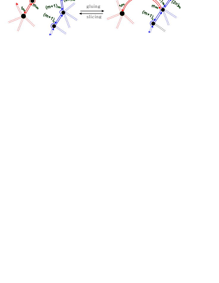
Figure 11. Lemma 2: gluing and slicing, the case $B^{I}_{g,n+1}$.

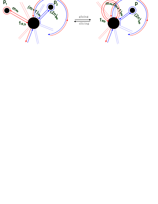
Figure 12. Lemma 2: gluing and slicing, the case $B^{II}_{g,n+1}$.

Proof.

Let $b=(L,\beta,\tau)$ be a planted bicellular map of genus $g$ having $n$ edges with plants $p_{1}$ and $p_{2}$ and tour $\beta\circ\tau=\omega_{1}\circ\omega_{2}$. Let

$$\omega_{1}=(1_{R_{b}},1_{b},\ldots,m_{b},m_{R_{b}})\quad\text{\rm and}\quad\omega_{2}=((m+1)_{R_{b}},(m+1)_{b},\ldots,2n_{b},2n_{R_{b}})$$

and $v_{i,b}$, for $1\leq i\leq J$ be the set of its vertices.

Consider the two vertices $(m_{R_{b}})$ and $v_{p_{2},b}$, where $(m_{R_{b}})$ is the plant $p_{1}$ and $v_{p_{2},b}$ denote the cycle containing half-edge $(m+1)_{R_{b}}$. I.e. we have

$$v_{p_{2},b}=(h^{1}_{p_{2},b},h^{2}_{p_{2},b},\ldots,h^{l}_{p_{2},b}),\quad\text{for \quad}l>0.$$

where $h^{1}_{p_{2},b}=\min v_{p_{2},b}$. Note that if $h^{1}_{p_{2},b}=\min v_{p_{2},b}=(m+1)_{R_{b}}$, then $v_{p_{2},b}$ is different from $v_{1,b}=(1_{R_{b}},\dots)$, whence $b\in B_{g,n}^{I}$ and if $h^{1}_{p_{2},b}=1_{R_{b}}$, then $v_{p_{2},b}=v_{1,b}$ and consequently $b\in B_{g,n}^{II}$.

The key operation consists in ”gluing ” $p_{1}=(m_{R_{b}})$ into $v_{p_{2},b}$. This generates the unicellular map, $\eta(b)$, with boundary component

(3.3) $$\gamma=\left((m+1)_{R_{b}},\underbrace{1_{R_{b}},1_{b},\dots,m_{b},m_{R_{b}}}_{\omega_{1}},(m+1)_{b},\dots,(2n)_{b},(2n)_{R_{b}}\right)$$

and the new vertex

$$w_{p_{2},b}=(h_{p_{2},b}^{1},m_{R_{b}},h_{p_{2},b}^{2},\ldots,h^{l}_{p_{2},b})\quad\text{where}\quad h^{1}_{p_{2},b}=(m+1)_{R_{b}},$$

obtained by gluing $(m_{R_{b}})$ into $v_{p_{2},b}$. Accordingly, $\eta(b)$ has vertex set

$$(\{v_{i,b}\mid 1\leq i\leq J\}\dot{\cup}\{w_{p_{2},b}\})\setminus\{v_{p_{2},b},(m_{R_{b}})\}.$$

Note that in case of $v_{1,b}\neq v_{p_{2},b}$, the gluing does not merge these $b$-vertices.

Suppose now $b\in B^{I}_{g,n}$. By definition there exists some $x\in\omega_{1}$ such that $\beta(x)\in\omega_{2}$. Thus there exists some $1_{R_{b}}<x<m_{R_{b}}$, such that $(m+1)_{R_{b}}<\beta(x)<2n_{R_{b}}$. Gluing produces the unicellular map $\eta(b)$ whose boundary component is given in eq. 3.3. We observe that the half-edges $1_{R_{b}}$ and $m_{R_{b}}$ map exactly to the half-edges $1$ and $\alpha(1)$ in $\eta(b)$ and furthermore, the half-edges $(m+1)_{b}$ to $2n_{R_{b}}$ map to $\eta(b)$-halfedges that are all greater than $\alpha(1)$. Consequently, there exists some $\eta(b)$ half-edge, $1<x<\alpha(1)$ such that $\alpha(x)>\alpha(1)$, whence $\eta(b)\in U^{I}_{g+1,n+1}$.

The case of $b\in B^{II}_{g,n}$ is analogous. Then there also exists some $1<x<\alpha(1)$ such that $\alpha(x)>\alpha(1)$ holds, whence $\eta(b)\in U^{II}_{g+1,n+1}$. In Fig. 11 and Fig. 12 we depict what happens if we glue $(m_{R_{b}})$ into $v_{p_{2},b}$ in these respective cases.

We next inspect that $\eta(b)$ has genus $(g+1)$. Indeed, $b$ satisfies $2-2g=v_{J}-n+2$, i.e. $2-2(g+1)=v_{J}-(n+1)+1$. Since the gluing transforms the $p_{1}$ plant into an edge, the latter equation shows that $\eta(b)$ has genus $(g+1)$.

We have thus shown that there exists a welldefined mapping

$$\eta\colon B^{I}_{g,n}\dot{\cup}\;B^{II}_{g,n}\longrightarrow U^{I}_{g+1,n+1}\dot{\cup}\;U^{II}_{g+1,n+1},$$

that induces by restriction the mappings

$$\eta_{I}\colon B^{I}_{g,n}\longrightarrow U^{I}_{g+1,n+1}\quad\text{\rm and}\quad\eta_{II}\colon B^{II}_{g,n}\longrightarrow U^{II}_{g+1,n+1}.$$

We next construct the inverse of $\eta$. To this end, let $u=(H,\alpha,\sigma)$ be a unicellular map of genus $g$ having $(n+1)$ edges with plant $p$ and face

(3.4) $$\gamma=\left((m+1)_{R_{b}},1_{R_{b}},1_{b},\dots,m_{b},m_{R_{b}},(m+1)_{b},\dots,(2n)_{b},(2n)_{R_{b}}\right),$$

where $1_{R_{b}}=1_{u}$, $\alpha(1_{u})=m_{R_{b}}$ and $\sigma$ having the $K$ cycles $v_{1,u},v_{2,u},\ldots,v_{K,u}$.

Figure 13. Constructing the inverse of $\eta$.

Suppose first $u\in U_{g+1,n+1}^{I}$, then $\{1_{R_{b}},\alpha(1_{R_{b}})\}$ is incident to two different vertices. We set

$$v_{1}=(h_{1}^{1},h_{1}^{2},h_{1}^{3},\ldots,h_{1}^{j})$$

where $h_{1}^{1}=(m+1)_{R_{b}}$ and

$$v_{2}=(h_{2}^{1},h_{2}^{2},\ldots,h_{2}^{l}),$$

where by definition $h_{2}^{1}=1_{R_{b}}$ and $\alpha(1_{R_{b}})=m_{R_{b}}$. Consequently, we have

$$h_{1}^{2}=\sigma(h_{1}^{1})=(\alpha\circ\gamma)(h_{1}^{1})=\alpha(1_{R_{b}})=m_{R_{b}}.$$

Second let $u\in U^{II}_{g+1,n+1}$. Then $\{1_{R_{b}},\alpha(1_{R_{b}})\}$ is incident to

$$v_{1}=(h_{1}^{1},h_{1}^{2},h_{1}^{3},\ldots,h_{1}^{j}),$$

such that $h_{1}^{1}=(m+1)_{R_{b}}$ and

$$h_{1}^{2}=(\alpha\circ\gamma)(h_{1}^{1})=\alpha(1_{R_{b}})=m_{R_{b}}.$$

Since $\alpha(1_{R_{b}})$ and $1_{R_{b}}$ are incident to the same vertex and $h_{1}^{2}=\alpha(1_{R_{b}})$, we can conclude that $1_{R_{b}}$ is a half-edge of $v_{1}$. In other words, there exist some half-edge $h_{1}^{a}$ (namely $h_{1}^{a}=1_{R_{b}}$), for some $1<a<j$, such that $\alpha(h_{1}^{a})=m_{R_{b}}$.

We now introduce the mapping $\varsigma$ obtained by “cutting” the edge $\{1_{R_{b}},\alpha(1_{R_{b}})\}$ in $u$. That is, $\varsigma$ splices $v_{1}$ into the two vertices

$$v_{p_{2},b} = (h_{1}^{1},h_{1}^{3},\ldots,h_{1}^{j})$$

$$p_{1} = (h_{1}^{2}).$$

This process generates the new vertex set

$$\{v_{i}\mid 1<i\leq K\}\cup\{v_{p_{2},b}\}\cup\{p_{1}\}.$$

Since $\alpha(1_{R_{b}})=m_{R_{b}}$, the sequence of half-edges

$$\omega_{1}=(1_{R_{b}},1_{b},2_{b},\dots,\alpha(1_{R_{b}}))$$

and

$$\omega_{2}=\left((m+1)_{R_{b}},(m+1)_{b},\dots,(2n)_{b},(2n)_{R_{b}}\right),$$

represent the two boundary components of the new map.
Furthermore, since for $u\in U^{I}_{g+1,n+1}\dot{\cup}\;U^{II}_{g+1,n+1}$, there exists some $k$, $1<k<\alpha(1)$, such that $\alpha(1)<\alpha(k)$. Since $u$ has the boundary component given in eq. (3.4), we have $1=1_{R_{b}}$ and $\alpha(1)=m_{b}$. Accordingly, there exists some $1_{R_{b}}<k<\alpha(1_{R_{b}})$, such that $\alpha(1_{R_{b}})<\alpha(k)$.

$\varsigma(u)$ has the two new boundary components $\omega_{1}$ and $\omega_{2}$, i.e. there exist some $k\in\omega_{1}$, such that $\beta(k)\in\omega_{2}$ and $\varsigma(u)$ is bicellular map. By construction, if $u\in U^{I}_{g+1,n+1}$, then $\varsigma(u)$ has its two plants incident to two distinct vertices, whence $\varsigma(u)\in B^{I}_{g,n}$. In case of $u\in U^{II}_{g+1,n+1}$ then $\varsigma(u)$ has its two plants incident to one vertex and $\varsigma(u)\in B^{II}_{g,n}$.

Euler’s characteristic formula implies that $g(u)=g(\varsigma(u))+1$. Furthermore, by construction,

$$\varsigma\circ\eta=\text{\rm id}_{B_{g,n}}\quad\text{\rm and}\quad\eta\circ\varsigma=\text{\rm id}_{{U^{I}_{g+1,n+1}}\dot{\cup}{U^{II}_{g+1,n+1}}}.$$

Thus $\eta$ is a bijection that induces by construction the bijections $\eta_{I}$ and $\eta_{II}$ and the lemma follows. ∎

4. The main result

Theorem 1.

Let $U_{g,n}$ and $B_{g,n}$ denote the sets of unicellular and bicellular maps containing $n$ edges and genus $g$. Then there is a bijection

(4.1) $$\beta\colon\dot{\bigcup}_{0\leq g_{1}\leq g+1,\;0\leq j\leq n}\left(U_{g_{1},j}\times U_{g+1-g_{1},n-j}\right)\;\dot{\cup}\;B_{g,n}\longrightarrow U_{g+1,n+1}.$$

Proof.

We have shown in Lemma 1 and Lemma 2 that there are bijections

$$\theta\colon\dot{\bigcup}_{0\leq g_{1}\leq g+1,\;0\leq j\leq n+1}\left(U_{g_{1},j}\times U_{g+1-g_{1},n-j}\right) \longrightarrow U^{III}_{g+1,n+1}$$

$$\eta\colon B_{g,n+1} \longrightarrow U^{I}_{g+1,n+1}\dot{\cup}\;U^{II}_{g+1,n+1}.$$

These two bijections determine

$$\beta\colon\dot{\bigcup}_{g_{1},j}\left(U_{g_{1},j}\times U_{g+1-g_{1},n-j}\right)\;\dot{\cup}\;B_{g,n}\longrightarrow U_{g+1,n+1},$$

whence the theorem. ∎

An immediate enumerative corollary of this bijection is the following result:

Corollary 1.

The generating function of unicellular and bicellular maps, ${\bf C}_{g}(z)$ and ${\bf C}_{g}^{[2]}(z)$ satisfy the following equation

(4.2) $$\sum_{g_{1}=0}^{g+1}\,{\bf C}_{g_{1}}(z){\bf C}_{g+1-g_{1}}(z)+{\bf C}_{g}^{[2]}(z)={\bf C}_{g+1}(z)/z,$$

which equivalent to the coefficient equation

(4.3) $$\sum_{g_{1}=0}^{g+1}\,\sum_{i\geq 0}^{n}\,{\sf c}_{g_{1}}(i){\sf c}_{g+1-g_{1}}(n-i)+{\sf c}_{g}^{[2]}(n)={\sf c}_{g+1}(n+1)$$

Corollary 1 can be proved using either (a) the matrix model [3, 11] and in particular the Schwinger-Dyson equation or (b) representation theory [10, 12].

References

- [1] J.E. Andersen, R.C. Penner, C.M. Reidys, and F.W.D. Huang. Topology of RNA-RNA interaction structures. J. Comput. Biol., 19(7):928–943, 2012.
- [2] J.E. Andersen, R.C. Penner, C.M. Reidys, and M.S. Waterman. Topological classification and enumeration of RNA structures by genus. J. Math. Biol., 2012.
- [3] F. Dyson. The s matrix in quantum electrodynamics. Phys. Rev., 75:1736, 1949.
- [4] F.W.D. Huang, W.W.J. Peng, and C.M. Reidys. Folding 3-noncrossing RNA pseudoknot structures. J. Comput. Biol., 16(11):1549–75, 2009.
- [5] F.W.D. Huang, J. Qin, C.M. Reidys, and P.F. Stadler. Partition function and base pairing probabilities for RNA-RNA interaction prediction. Bioinformatics., 25(20):2646–2654, 2009.
- [6] F.W.D. Huang, J. Qin, C.M. Reidys, and P.F. Stadler. Target prediction and a statistical sampling algorithm for RNA-RNA interaction. Bioinformatics, 26:175–181, 2010.
- [7] M. Loebl and I. Moffatt. The chromatic polynomial of fatgraphs and its categorification. Adv. Math., 217:1558–1587, 2008.
- [8] R.C. Penner, M. Knudsen, C. Wiuf, and J.E. Andersen. Fatgraph models of proteins. Comm. Pure Appl. Math., 63:1249–1297, 2010.
- [9] C.M. Reidys, F.W.D. Huang, J.E. Andersen, R.C. Penner, P.F. Stadler, and M.E. Nebel. Topology and prediction of RNA pseudoknots. Bioinformatics., 27(8):1076–1085, 2011.
- [10] B. E. Sagan. The Symmetric Group: Representations, Combinatorial Algorithms, and Symmetric Functions. Springer-Verlag, New York, 2001.
- [11] J. Schwinger. On Green’s functions of quantized fields I+II. Proc. Natl. Acad. Sci, 37:452–459, 1951.
- [12] D. Zagier. On the distribution of the number of cycles of elements in symmetric groups. Nieuw Arch. Wiskd., IV. Ser., 13(3):489–495, 1995.