CIJET: a program for computation of jet cross sections induced by quark contact interactions at hadron colliders

Abstract

We describe CIJET1.0, a Fortran program that aiming for the calculation of single-inclusive jet or dijet production cross sections induced by quark contact interactions from new physics at hadron colliders, up to next-to-leading order in QCD. It covers various contact interactions with different chiral and color structures. The code is designed in a way that could be used for fast calculations with arbitrary parton distribution functions based on interpolations of the QCD coupling constant and parton distribution functions.

PROGRAM SUMMARY

Manuscript Title: CIJET1.0: a program for computation of jet cross sections induced by quark contact interactions at hadron colliders
Authors: Jun Gao
Program Title: CIJET 1.0
Journal Reference:
Catalogue identifier:
Preprint number: SMU-HEP-13-08
Licensing provisions: none
Programming language: Fortran; with some included libraries coded in C
Computer: all
Operating system: any UNIX-like system
RAM: $\sim$ 300 MB
Supplementary material:
Keywords: Jet production; Quark compositeness; Perturbative calculation; Hadron colliders
Classification: 11.1
Nature of problem: Calculation of single-inclusive jet and dijet cross sections induced by quark contact interactions up to next-to-leading order in QCD at hadron colliders.
Solution method: Using the VEGAS Monte Carlo sampling and subtracted matrix element to generate weight grids and store them in a table file that allows for later interpolations on arbitrary parton distribution functions.
Running time: Depends on details of the calculation and the required numerical accuracy.

1 Introduction

Jet production at hadron colliders provides an excellent opportunity to test perturbative QCD (PQCD) and to search for possible new physics (NP) beyond the Standard Model (SM) over a wide range of energy scales. Invariant mass distributions of the dijets [1], dijet angular distributions [2, 3, 4], inclusive jet $p_{T}$ distribution [5], and other jet observables at the LHC [6] have already extended current searches for quark compositeness, excited quarks, and other new particle resonances toward the highest energies attainable. Among all these measurements, the inclusive jet $p_{T}$ distribution and dijet angular distribution show a great sensitivity to possible quark contact interactions (CIs) induced by new physics models. In the SM, Quantum Chromodynamics (QCD) predicts the jets are preferably produced in large rapidity region, via small angle scattering in $t$-channel processes. Also the production rates fall off rapidly in large $p_{T}$ or large dijet invariant mass region. On the contrary, the jet production induced by quark contact interactions is expected to be much more isotropic and fall off slower as the increasing of jet $p_{T}$ or dijet invariant mass, and thus the distributions at the LHC could be largely modified.

The measurement of quark contact interactions has been used to set limits on the quark composite models which have been studied extensively in the literature [7, 8]. It is assumed that quarks are composed of more fundamental particles with new strong interactions at a compositeness scale $\Lambda$, much greater than the quark mass scales. At the energy well below $\Lambda$, quark contact interactions are induced by the underlying strong dynamics, and yield observable signals at hadron colliders. The newest bounds of $\Lambda$ at the $95\%$ confidence level (C.L.) from the CMS collaboration are around $10\,{\rm TeV}$ based on $2.2\,{\rm fb}^{-1}$ collected data of the dijet angular measurement [4] and $5\,{\rm fb}^{-1}$ data of the single-inclusive jet measurement [5]. Previous limits from the Tevatron and LHC can be found in Refs. [2, 3, 9, 10].

In our earlier studies [11], we presented the theoretical calculations of the next-to-leading (NLO) order QCD corrections to the dijet production induced by quark CIs, which are used by the experimentalists to set constraints on the quark compositeness scales [4]. In this work we summarize the numerical program used for the dijet calculation with extensions for the calculation of single-inclusive jet production, which will be used in the upcoming measurement [5]. One common issue of the experimental analyses at the hadron colliders is that, they require massive repetitive calculations using different parton distribution functions (PDFs) to estimate the theoretical uncertainties. And fast calculation algorithms for arbitrary PDFs, like the implementations of FastNLO [12] and APPLGRID [13] are highly desirable. Thus in our program we further provide a fast interpolation modular that allows for the calculations of using arbitrary PDFs within seconds while maintaining the desirable numerical accuracy.

This document is structured as follows: Section 2 briefly summarizes the theoretical model and calculations. Section 3 describes the fast interpolation algorithm used. And Section 4-6 show the inputs, running, and outputs of the program. Section 7 shows some sample results from the program and Section 8 is a conclusion.

2 Jet cross sections and quark contact interactions

We consider a subset of quark contact interactions that are the products of electroweak isoscalar quark currents which are assumed to be flavor-symmetric to avoid large flavor-changing neutral-current interactions [8]. The effective Lagrangian can be written as

$$\mathcal{L}_{NP}=\frac{1}{2\Lambda^{2}}\sum_{i=1}^{6}c_{i}O_{i},$$ (1)

where $\Lambda$ is the new physics scale, $c_{i}$ are Wilson coefficients. And the operators $O_{i}$ in chiral basis are given by

$$O_{1} = \delta_{ij}\delta_{kl}\left(\sum_{c=1}^{3}\bar{q}_{Lci}\gamma_{\mu}q_{Lcj}\sum_{d=1}^{3}\bar{q}_{Ldk}\gamma^{\mu}q_{Ldl}\right),$$

$$O_{2} = {\rm T}_{ij}^{a}{\rm T}_{kl}^{a}\left(\sum_{c=1}^{3}\bar{q}_{Lci}\gamma_{\mu}q_{Lcj}\sum_{d=1}^{3}\bar{q}_{Ldk}\gamma^{\mu}q_{Ldl}\right),$$

$$O_{3} = \delta_{ij}\delta_{kl}\left(\sum_{c=1}^{3}\bar{q}_{Lci}\gamma_{\mu}q_{Lcj}\sum_{d=1}^{3}\bar{q}_{Rdk}\gamma^{\mu}q_{Rdl}\right),$$

$$O_{4} = {\rm T}_{ij}^{a}{\rm T}_{kl}^{a}\left(\sum_{c=1}^{3}\bar{q}_{Lci}\gamma_{\mu}q_{Lcj}\sum_{d=1}^{3}\bar{q}_{Rdk}\gamma^{\mu}q_{Rdl}\right),$$

$$O_{5} = \delta_{ij}\delta_{kl}\left(\sum_{c=1}^{3}\bar{q}_{Rci}\gamma_{\mu}q_{Rcj}\sum_{d=1}^{3}\bar{q}_{Rdk}\gamma^{\mu}q_{Rdl}\right),$$

$$O_{6} = {\rm T}_{ij}^{a}{\rm T}_{kl}^{a}\left(\sum_{c=1}^{3}\bar{q}_{Rci}\gamma_{\mu}q_{Rcj}\sum_{d=1}^{3}\bar{q}_{Rdk}\gamma^{\mu}q_{Rdl}\right),$$ (2)

in which $c$, $d$ are generation indices and $i$, $j$, $k$, $l$, $a$ are color indices, and ${\rm T}^{a}$ are the Gell-Mann matrices with the normalization ${\rm Tr}({\rm T}^{a}{\rm T}^{b})=\delta^{ab}/2$. Beside of the quark compositeness, the above interactions can also arise from various kinds of new physics models, induced by the exchange of new heavy resonances, such as $Z^{\prime}$ models [14] and extra dimensions models [15].

The jet cross sections (up to NLO) in each kinematic bin, depending on the scale $\Lambda$ and Wilson coefficients $c_{i}$ at input scale $\Lambda$, can be expressed as

$$\sigma_{bin} = \sum_{i=1}^{6}(\lambda_{i}(b_{i}+a_{i}r))/\Lambda^{2}+\sum_{i=1}^{6}(\lambda_{i}^{2}(b_{ii}+a_{ii}r))/\Lambda^{4}$$ (3)

$$+\sum_{i=1,3,5}(\lambda_{i}\lambda_{i+1}(b_{ii+1}+a_{ii+1}r))/\Lambda^{4}$$

$$+\sum_{i=1,2,5,6}(\lambda_{i}\lambda_{4}(b_{i4}+a_{i4}r))/\Lambda^{4}.$$

with $\lambda_{i}$ defined by $c_{i}=4\pi\lambda_{i}$, $r=\ln(\Lambda/\mu_{0})$, and $\mu_{0}$ is an arbitrary reference scale chosen according to the kinematic range of the bin (not the same as QCD scales). All $a$’s vanish at leading order (LO). Since QCD interaction preserves parity, we should have $b(a)_{1,2}=b(a)_{5,6}$, $b(a)_{11,22,12}=b(a)_{55,66,56}$, and $b(a)_{14,24}=b(a)_{54,64}$. More details of the theoretical calculations can be found in [11].

3 Grid interpolation

In general, dependence of the jet cross sections on the PDF and the QCD coupling constant $\alpha_{s}$ can be expressed as

$$\sigma_{bin}=\sum_{i,j}\int dx_{1}dx_{2}f_{i/h_{1}}(x_{1},\mu_{f})f_{j/h_{2}}(x_{2},\mu_{f})\sum_{p}\alpha_{s}^{p}(\mu_{r})\mathcal{B}_{p}(x_{1},x_{2};\mu_{f},\mu_{r}),$$ (4)

where $i,j$ are the parton flavors, $p$ indicates the order of $\alpha_{s}$, and $\mu_{f(r)}$ are the factorization and renormalization scales. We choose a 3-dimensional grid of $x_{1}-x_{2}-\mu_{f}$ with $N_{x}\times N_{x}\times N_{q}$ grid points, which are uniformly spaced in $x_{1}^{\delta}$, $x_{2}^{\delta}$ and $\ln\ln{\mu_{f}/Q_{0}}$ with $\delta=0.3$ and $Q_{0}=0.3$ GeV. We choose $N_{x}=30$ and $N_{q}=15$ which are found to be good enough with an interpolation accuracy of about 0.1%. Both ends of each dimension are determined according to the kinematic range of the bin considered. We use a fourth-order interpolation and rewrite the cross section as

$$\sigma_{bin}=\sum_{p,k}\sum_{n_{1},n_{2},n_{3}}I_{k,p}(n_{1},n_{2},n_{3},\xi)(\alpha_{s}^{p}(\xi\mu_{f})\Phi_{k})|_{n_{1},n_{2},n_{3}},$$ (5)

where $\xi=\mu_{r}/\mu_{f}$, and $n_{i}$ are indices of grid points. The sum is performed over the perturbative expansion order of QCD coupling constant ($p$) and the parton luminosities ($k$). The parton luminosities involved here for up to NLO calculations are

$$\Phi_{1} =\sum_{ij={qq^{\prime}},{\bar{q}\bar{q}^{\prime}}}x_{1}^{2}x_{2}^{2}f_{i/h_{1}}(x_{1},\mu_{f})f_{j/h_{2}}(x_{2},\mu_{f}),$$

$$\Phi_{2} =\sum_{ij={qq},{\bar{q}\bar{q}}}x_{1}^{2}x_{2}^{2}f_{i/h_{1}}(x_{1},\mu_{f})f_{j/h_{2}}(x_{2},\mu_{f}),$$

$$\Phi_{3} =\sum_{ij={q\bar{q}^{\prime}}}x_{1}^{2}x_{2}^{2}f_{i/h_{1}}(x_{1},\mu_{f})f_{j/h_{2}}(x_{2},\mu_{f})+(h_{1}\leftrightarrow h_{2}),$$

$$\Phi_{4} =\sum_{ij={q\bar{q}}}x_{1}^{2}x_{2}^{2}f_{i/h_{1}}(x_{1},\mu_{f})f_{j/h_{2}}(x_{2},\mu_{f})+(h_{1}\leftrightarrow h_{2}),$$

$$\Phi_{5} =\sum_{ij={gq},{g\bar{q}}}x_{1}^{2}x_{2}^{2}f_{i/h_{1}}(x_{1},\mu_{f})f_{j/h_{2}}(x_{2},\mu_{f})+(h_{1}\leftrightarrow h_{2}).$$ (6)

Note that the $gg$ luminosity does not contribute to the cross sections induced by quark contact interactions up to NLO. In the code the grid coefficients $I_{k,p}(n_{1},n_{2},n_{3},\xi)$ with dependence on $\xi$ solved analytically, are calculated and stored in a table file for each kinematic bin, which allows fast interpolations of $\sigma_{bin}$ for arbitrary PDF and renormalization scale choices. The grid interpolation we used here is based on the original approaches introduced by FastNLO [12] and APPLGRID [13], but with slightly modifications to adapt for our calculation.

4 Program inputs

The input parameters are specified in the files with the extension .card in the subdirectory data. Each line contains a record for an input variable: a character tag with the name of the variable, followed by the variable’s value and descriptions.

proinput.card contains various switches that

• pdf is the name of the PDF file read from LHAPDF [16] used in the calculation, e.g., CT10.LHgrid for CT10 NLO PDFs [17]. Since the code has a fast PDF interpolation interface in the final step, user can also change the PDF choice there.

• pdfmember specifies the PDF member used in the calculation as appearing in LHAPDF, e.g., 0 for central PDF.

• ang specifies the two observables of the kinematic bin. Basically the program calculates the total cross section in two-dimentional kinematic bins. For ang=1-3, the first observable of the bin is always the dijet invariant mass. The second observable is $\chi=\exp(|y_{1}-y_{2}|)$ for ang=1, $y^{*}=|y_{1}-y_{2}|/2$ for ang=2, and $y_{max}=\max(|y_{1}|,|y_{2}|)$ for ang=3. While ang=4 is for single-inclusive jet production with the first observable as $p_{T}$ of the individual jet and second as absolute rapidity $|y|$ of the individual jet.

• mode=fitll/fitcs/fital controls the calculation scheme. The code first calculates the coefficients ($a,b$) defined in Eq. (3) at both LO and NLO. The differences between the three choices are that fitll assumes only left-handed color-singlet operator at input scale (coupling $c_{1}$). And fitcs includes all the color-singlet operators at input scale (couplings $c_{1}$, $c_{3}$, $c_{5}$). fital considers all the six operators in Eq. (1). User can choose the calculation scheme according to the model studied since the most general case mode=fital consumes much more CPU times.

• pseed specifies the random-number seed used by the Monte Carlo integration.

• many is the number of Monte Carlo sampling points specified for the calculation. User may need to adjust it according to the numerical accuracy required. For an accuracy of a few per mille, recommendation is 3,000,000 or more.

• ppcollider represents the type of the collider. 0 for $p\bar{p}$ machine and 1 for $pp$ machine.

• Sqrts gives the center-of-mass energy $\sqrt{s}$ of the collider in GeV.

• scalescheme specifies the choice of the hard momentum scale that defines the central value of the factorization and renormalization scales. For dijet production (ang=1-3), 0 corresponds to choose the central value as average $p_{T}$ of the two leading jets, and 1 corresponds to choose the central value as $\exp(0.3y^{*})$ times the harder jet $p_{T}$ in the two leading jets. While for single-inclusive jet production, 0 indicates using the individual jet $p_{T}$ as the central value, and 1 for using maximum jet $p_{T}$ in the rapidity region as the central value.

kininput.dat contains parameters for clustering and selection of jets, in the same format as in proinput.card.

• jetscheme specifies the jet algorithm used in the calculations: 1 for the anti-$k_{T}$ jet algorithm [18], 2 for the cone algorithms [19], with Rsep=1.3 for modified Snowmass, and Rsep=2 for midpoint algorithm. Note here for the NLO calculation the anti-$k_{T}$ algorithm is equivalent to the $k_{T}$ [20] or Cambridge-Aachen [21] algorithm.

• recscheme sets the recombination scheme [22] used in jet clustering: 2 is for the 4-momentum scheme (recommended for LHC), and 1 for the $E_{T}$ scheme.

• Rcone sets the distance parameter or cone size for the jet algorithm used.

• Rsep is only active for cone algorithm as explained above.

• ycut and ptcut specify conditions for jet acceptance, i.e., the maximal rapidity and lowest $p_{T}$ (in GeV) for a cluster to be considered as a jet.

• yb, ys specify the upper limit on $y_{boost}=|y_{1}+y_{2}|/2$ and $y^{*}$ of the dijet system, respectively, and are not used for calculations of single-inclusive jet production.

bininput.card sets up a scan of the two-dimensional bin. Under tagged line massbin, user can specify one invariant mass (or $p_{T}$) bin per line, containing the lower and upper limits (in GeV). And under tagged line rapbin, user can write one angular bin per line (corresponding to $\chi$, $y^{*}$, $y_{max}$, or $|y|$ depending on ang). The code will do a scan over all the two-dimensional bins specified.

5 Compilation and running

After unzip the source file, go to the main directory and run make. The executables will be generated and moved into directory data. The program uses the VEGAS subroutine from CUBA library [23] for the Monte Carlo integration.

There are two main executables. dijets4ci_sin is for the calculation using a single CPU core. And dijets4ci_mul is for the calculation using multicore which is much faster. Before runing dijets4ci_mul, user needs to first set the number of cores used by running source setcores.sh $1, where $1 is the number. Otherwise dijets4ci_mul will use all the cores available. To run the code simply by entering ./dijets4ci_sin $tag or ./dijets4ci_mul $tag under the data directory, where $tag specifies the name of the job. Note that during the run the code needs to write into some auxiliary files for the parellel calculation. Also users are suggested to use reasonable amount of cores since it costs additional times for the master process to combine results from each cores. Besides, there are another two executables in fastCI directory, i.e., ciconv and cixsec, which will be explained later.

6 Program outputs

At the end of each run, the program generates an output file $tag_fitresults.dat containing the calculated coefficients in Eq. (3) for the specified PDF, 6 groups in total for each bin (LO and NLO with 3 scale choices). Note that the value of $\mu_{0}$ for each bin are also written into the output file.

At the same time, the gird files (one for each bin) are generated and stored in the fastCI/fgrid directory. Under fastCI directory, user can first run ./ciconv $1 $2 $3 $4 to calculate the coefficients for arbitrary PDFs and scale choices, where argument $1 is the PDF file name, $2 is the number of PDF member, $3 is the grid file name as in fgrid directory, and $4 is the specified file name for the output. The calculated coefficients, 18 groups for each bin (LO and NLO with 9 scale choices), are written into file $4. Using the coefficients, as well as $\mu_{0}$ value in $4, user can calculate the cross sections for arbitrary scale $\Lambda$ and Wilson coefficients $c_{i}$ according to Eq. (3). Or user can run ./cixsec $1 $2 to get the cross sections for $\Lambda$ and $\lambda_{i}$ values specified in file input, where $1 is the output from ciconv, and the cross sections are written into $2.

7 Sample results

In this section we present some representative sample results from the program for both single-inclusive jet and dijet production at LHC 8 TeV. For simplicity we just show results for a single model with $\Lambda=7$ TeV and vector-like color-singlet coupling, $\lambda_{1,5}=-1$, $\lambda_{3}=-2$, $\lambda_{2,4,6}=0$. We use the anti-$k_{T}$ jet algorithm with $R=0.7$ for single-inclusive jet production and $R=0.6$ for dijet production. The scalescheme is set to 0 for single-inclusive jet production and 1 for dijet production. And we only present the differential cross sections in the central rapidity region, i.e., $|y|<0.5$ or $|y^{*}|<0.5$ for single-inclusive jet and dijet production, which is preferred by the contributions from CIs. In Fig. 1 we show comparisons of the LO and NLO jet cross sections. The NLO QCD corrections are found to reduce the cross sections in most of the cases except for the extremely large $p_{T}$ or large invariant mass region. Also in Fig. 1 we plot the ratios of the cross sections that directly from the numerical integration and from latter interpolations. We can see very good agreements between them, and the interpolation only introduces numerical errors of the order 0.1%, which are negligible in current analyses.

Using the fast interpolation we can obtain the results for arbitrary scale and PDF choices without redoing the numerical integration, which is the most time consuming part. In Fig. 2 we plot the scale variation envelope of the jet cross sections by varying the factorization and renormalization scales independently around the central value by a factor of two. The cross sections are normalized to the LO or NLO predictions using the central scale value. We can see that the NLO corrections greatly reduce the scale uncertainties, especially the factorization scale uncertainties, for both cases, which makes the theoretical predictions more reliable. Furthermore, in Fig. 3 we compare the NLO predictions with 68% C.L. PDF errors from CT10 [17], MSTW2008 [24], and NNPDF2.3 [25] NLO PDFs. CT10 gives higher predictions in both cases, and MSTW2008 shows much smaller PDF uncertainties in the extremely large $p_{T}$ and large invariant mass region.

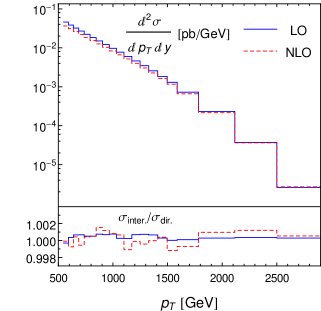
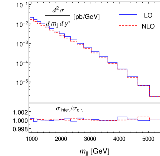
Figure 1: Jet cross sections induced by the CIs at both LO and NLO, using the central scale choice and CT10 NLO PDF. Ratios between the results directly from the numerical integration and the results from latter interpolation using the weight grids are also shown. Left and right panel correspond to single-inclusive jet and dijet production respectively.

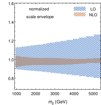
Figure 2: Scale uncertainty envelope of the jet cross sections induced by the CIs at both LO and NLO normalized to the central scale predictions, using the CT10 NLO PDF. Left and right panel correspond to single-inclusive jet and dijet production respectively.

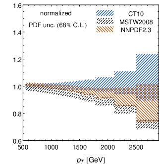
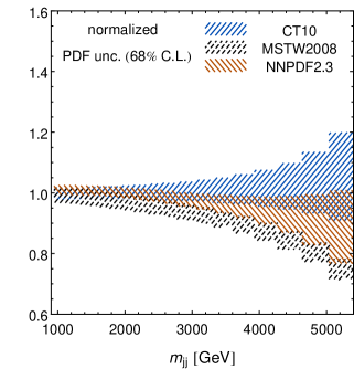
Figure 3: PDF uncertainties of the jet cross sections induced by the CIs at NLO normalized to the CT10 central predictions, using the central scale choice. Results are shown for CT10, MSTW2008 and NNPDF2.3 NLO PDFs. Left and right panel correspond to single-inclusive jet and dijet production respectively.

8 Conclusions

In conclusion, this document describes the CIJET1.0 program that aiming for the calculation of single-inclusive jet or dijet production cross sections induced by quark contact interactions from new physics at hadron colliders, up to NLO in QCD. It covers various contact interactions with different chiral and color structures. The program allows for parellel calculations of the numerical integrations using the CUBA library. Moreover, the program includes a fast interpolation modular that could be used for calculations with arbitrary parton distribution functions without redoing the time consuming numerical integrations. The program could be used for the experimental analyses of the quark compositeness at the LHC.

References

- [1] S. Chatrchyan et al. [CMS Collaboration], Phys. Lett. B 704, 123 (2011).
- [2] V. Khachatryan et al. [CMS Collaboration], Phys. Rev. Lett. 106, 201804 (2011);
- [3] G. Aad et al. [ATLAS Collaboration], New J. Phys. 13, 053044 (2011).
- [4] S. Chatrchyan et al. [CMS Collaboration], JHEP 1205, 055 (2012).
- [5] S. Chatrchyan et al. [ CMS Collaboration], arXiv:1301.5023 [hep-ex].
- [6] G. Aad et al. [Atlas Collaboration], Eur. Phys. J. C 71, 1512 (2011); S. Chatrchyan et al. [CMS Collaboration Collaboration], Phys. Lett. B 700, 187 (2011); S. Chatrchyan et al. [CMS Collaboration], Phys. Rev. Lett. 107, 132001 (2011).
- [7] E. Eichten, K. D. Lane and M. E. Peskin, Phys. Rev. Lett. 50, 811 (1983); E. Eichten, I. Hinchliffe, K. D. Lane and C. Quigg, Rev. Mod. Phys. 56, 579 (1984) [Addendum-ibid. 58, 1065 (1986)]; P. Chiappetta and M. Perrottet, Phys. Lett. B 253, 489 (1991); O. Domenech, A. Pomarol and J. Serra, Phys. Rev. D 85, 074030 (2012).
- [8] K. D. Lane, arXiv:hep-ph/9605257.
- [9] F. Abe et al. [CDF Collaboration], Phys. Rev. Lett. 77, 5336 (1996) [Erratum-ibid. 78, 4307 (1997)]; T. Aaltonen et al. [CDF Collaboration], Phys. Rev. D 79, 112002 (2009); V. M. Abazov et al. [D0 Collaboration], Phys. Rev. Lett. 103, 191803 (2009).
- [10] G. Aad et al. [ATLAS Collaboration], Phys. Lett. B 694, 327 (2011); V. Khachatryan et al. [CMS Collaboration], Phys. Rev. Lett. 105, 262001 (2010).
- [11] J. Gao, C. S. Li, J. Wang, H. X. Zhu and C. P. Yuan, Phys. Rev. Lett. 106, 142001 (2011); J. Gao, C. S. Li and C. P. Yuan, JHEP 1207, 037 (2012).
- [12] T. Kluge, K. Rabbertz, and M. Wobisch, hep-ph/0609285; M. Wobisch et al. [fastNLO Collaboration], arXiv:1109.1310 [hep-ph].
- [13] T. Carli, D. Clements, A. Cooper-Sarkar, C. Gwenlan, G. P. Salam, F. Siegert, P. Starovoitov and M. Sutton, Eur. Phys. J. C 66, 503 (2010).
- [14] P. Langacker, Rev. Mod. Phys. 81, 1199 (2008).
- [15] L. Randall and R. Sundrum, Phys. Rev. Lett. 83, 3370 (1999) .
- [16] M. R. Whalley, D. Bourilkov, and R. C. Group, hep-ph/0508110. The latest LHAPDF library can be downloaded from http://hepforge.cedar.ac.uk/lhapdf/ .
- [17] H. -L. Lai, M. Guzzi, J. Huston, Z. Li, P. M. Nadolsky, J. Pumplin and C. -P. Yuan, Phys. Rev. D 82, 074024 (2010).
- [18] M. Cacciari, G. P. Salam, and G. Soyez, JHEP 04 (2008) 063.
- [19] G. C. Blazey et. al., hep-ex/0005012.
- [20] S. Catani, Y. L. Dokshitzer, M. H. Seymour, and B. R. Webber, Nucl. Phys. B406 (1993) 187; S. D. Ellis and D. E. Soper, Phys. Rev. D48 (1993) 3160.
- [21] Y. L. Dokshitzer, G. D. Leder, S. Moretti and B. R. Webber, JHEP 08 (1997) 001.
- [22] G. P. Salam, Eur. Phys. J. C67 (2010) 637.
- [23] T. Hahn, Comput. Phys. Commun. 168 (2005) 78.
- [24] A. D. Martin, W. J. Stirling, R. S. Thorne and G. Watt, Eur. Phys. J. C 63, 189 (2009).
- [25] R. D. Ball, V. Bertone, S. Carrazza, C. S. Deans, L. Del Debbio, S. Forte, A. Guffanti and N. P. Hartland et al., Nucl. Phys. B 867, 244 (2013).