Technical Report: A Receding Horizon Algorithm for Informative Path Planning with Temporal Logic Constraints

Abstract

This technical report is an extended version of the paper ’A Receding Horizon Algorithm for Informative Path Planning with Temporal Logic Constraints’ accepted to the 2013 IEEE International Conference on Robotics and Automation (ICRA).

This paper considers the problem of finding the most informative path for a sensing robot under temporal logic constraints, a richer set of constraints than have previously been considered in information gathering. An algorithm for informative path planning is presented that leverages tools from information theory and formal control synthesis, and is proven to give a path that satisfies the given temporal logic constraints. The algorithm uses a receding horizon approach in order to provide a reactive, on-line solution while mitigating computational complexity. Statistics compiled from multiple simulation studies indicate that this algorithm performs better than a baseline exhaustive search approach.

I Introduction

In this paper we propose an algorithm for controlling a mobile sensing robot to collect the most valuable information in its environment, while simultaneously carrying out a required sequence of actions described by a temporal logic (TL) specification. Our algorithm is useful in situations where a robot’s main objective is to collect information, but it must also perform pre-specified actions for the sake of safety or reliability. Consider searching for a survivor trapped in the rubble of a collapsed building. Our algorithm would drive the robot to locate the survivor while avoiding obstacles, and returning to a rescue worker to report on the progress of its search. The obstacle avoidance and visit to the worker are represented as temporal logic constraints. In order to locate the survivor, the robot plans a path on-line, in a receding horizon fashion, such that it localizes the survivor as precisely as possible, while still satisfying the temporal logic constraints.

This work brings together methods from information theory and formal control synthesis to create new tools for robotic information gathering under complex constraints. More specifically, the robot uses a recursive Bayesian filter to estimate the quantity of interest in its environment (e.g. the location of a survivor) from its noisy sensor measurements. The Shannon entropy of the Bayesian estimate is used as a measure of the robot’s uncertainty about the quantity of interest. The robot plans a path to maximally decrease the expected entropy of its estimate over a finite time horizon, subject to the TL constraints. The path planning is repeated at each time step as the Bayesian filter is updated with new sensor measurements to give a reactive, receding horizon planner. Our algorithm is guaranteed to satisfy the TL specification. We compare the performance of our algorithm to a non-reactive, exhaustive search method. We show in statistics compiled from extensive simulations that our receding horizon algorithm gives a lower entropy estimate with lower computational complexity than the exhaustive search method.

The algorithm we present is applicable to many scenarios in which we want a robot to gather informative data, but where safety and reliability are critical. For example, our algorithm can be used by a mobile robot deployed on Mars that is tasked with collecting soil samples and images while gathering enough sunlight to charge its batteries and avoiding dangerous terrain. In an animal population monitoring scenario, our algorithm can drive a robot to count animals of a given species whose positions are unknown while avoiding sensitive flora and fauna, eventually uploading data to scientists. Our algorithm could also be used, for example, in active SLAM to control a robot to build a minimum uncertainty map [22] of its environment while avoiding walls and returning to a base station for charging.

Extensive work already exists in using information theoretic tools in robotic information gathering applications. Most of this work uses a one-step-look-ahead approach [5, 18], a receding horizon approach [8, 4], or an offline plan based on the sub-modularity property of mutual information [21, 20, 16]. The key innovation in our algorithm is that it gives a path which is guaranteed to satisfy rich temporal logic constraints. Temporal logic constraints can specify complex, layered temporal action sequences that are considerably more expressive than the static constraints considered in previous works. Indeed, much of the work in constrained informative path planning can be phrased as a special case of the TL constraints that we consider here. For example the authors of [4] solve an information-gathering problem in which an underwater agent must avoid high traffic areas and communicate with researchers—constraints which can be naturally expressed as TL statements.

In this work, we consider a particular kind of temporal logic called syntactically co-safe linear temporal logic (scLTL) [12]. Synthesis of trajectories from scLTL specifications is currently an active area of research [1, 3], as is the use of receding horizon control to solve optimization problems over TL-constrained systems. Receding horizon control (RHC), sometimes referred to as model-predictive control, is a control technique in which current information is used to predict performance over a finite horizon [14, 17]. The authors of [23] use a receding horizon path planning algorithm that satisfies TL constraints in a provably correct manner and is capable of correcting navigational errors on-line. In [7], the authors extended this principle to provide a receding horizon algorithm for gathering time-varying, deterministic rewards in a TL-constrained system. The analysis of our informative planning algorithm was inspired by [7], with the significant difference that information gain is a stochastic quantity which depends on noisy sensor measurements.

The paper is outlined as follows. We define the necessary mathematical preliminaries in Section II. In Section III, we formalize the scLTL-constrained informative path planning problem. In Section IV we present our receding horizon algorithm, and prove that it satisfies the scLTL constraints. Results from simulations comparing our algorithm to a baseline exhaustive search method are presented in Section V. Finally, in Section VI, we give our conclusions and discuss directions for future work.

As mentioned in the abstract, this report is an extended version of a paper accepted to the 2013 ICRA conference. The main additions are some information theory definitions in Section II and a proof of Theorem 1 in Section IV.

II Notation and definitions

For a set $S$, we use $|S|$ and $2^{S}$ to denote its cardinality and power set, respectively. $S\times T$ is the Cartesian product of $S$ and $T$.

II-A Information theory

Information theory is a general mathematical theory of communication [19]. In this work we borrow from information theory measures of uncertainty and information content of discrete random variables.

We denote the range space of a discrete random variable $X$ as $R_{X}$, its realization as $x\in R_{X}$, and its probability mass function (pmf) as $p_{X}$. The Shannon entropy [19] (referred to in the sequel as simply “entropy”) of a discrete random variable $X$ is

$$H(X)=H(p_{X})=-\sum_{x\in R_{X}}p_{X}(x)\log(p_{X}(x)).$$ (1)

The logarithm in (1) is base 2 by convention and entropy is measured in units of “bits”. The entropy of a random variable is a measure of its “randomness” or “uncertainty”. For a fixed range space $R_{X}$, $H(X)\in[0,\log(|R_{X}|)]$. A uniformly distributed random variable achieves the upper bound and a deterministic variable achieves the lower bound.

For two discrete random variables $X$ and $Y$, the conditional entropy [6] of $X$ given $Y$ is

$$\begin{split}H(X|Y)=&H(p_{X}|p_{Y})\\ =&-\sum_{y\in R_{Y}}\sum_{x\in R_{X}}p_{X,Y}(x,y)\log(p_{X|Y}(x|y)).\end{split}$$ (2)

In general, $H(X|Y)\in[0,H(X)]$. $H(X|Y)$ is a measure of how random $X$ is if we are given knowledge of $Y$ and the statistical relationship between $X$ and $Y$.

The mutual information [6] between two random variables is

$$\begin{split}I(X;Y)=&I(p_{X};p_{Y})\\ =&\sum_{x\in R_{X}}\sum_{y\in R_{Y}}p_{X,Y}(x,y)\log(\frac{p_{X,Y}(x,y)}{p_{X}(x)p_{Y}(y)}).\\ \end{split}$$ (3)

The identity $I(X;Y)=H(X)-H(X|Y)$ leads to the natural interpretation of mutual information as the increase in certainty of $X$ when we have knowledge of $Y$.

II-B Transition systems and syntactically co-safe LTL

A weighted transition system [2] is a tuple $TS=(Q,q_{0},Act,Trans,AP,L,d)$, where $Q$ is a set of states, $q_{0}\in Q$ is the initial state, $Act$ is a set of actions, $Trans\subseteq Q\times Act\times Q$ is a transition relation, $AP$ is a set of atomic propositions, $L:Q\to 2^{AP}$ is a labeling function of states to atomic propositions, and $d:Trans\to\mathbb{R}$ is a weighting function over the set of transitions.

A finite state automaton (FSA) is a tuple $\mathcal{A}=(\Sigma,\Pi,\Sigma_{0},F,\Delta_{\mathcal{A}})$ where $\Sigma$ is a finite set of states, $\Pi$ is an input alphabet, $\Sigma_{0}\subseteq\Sigma$ is a set of initial states, $F\subseteq\Sigma$ is a set of final (accepting) states, and $\Delta_{\mathcal{A}}\subseteq\Sigma\times\Pi\times\Sigma$ is a deterministic transition relation.

An accepting run $r_{\mathcal{A}}$ of an automaton $\mathcal{A}$ on a finite word $w=w^{0}w^{1}\ldots w^{j}$ over $\Pi$ is a sequence of states $r_{\mathcal{A}}=\sigma^{0}\sigma^{1}\ldots\sigma^{j+1}$ such that $\sigma^{j+1}\in F$ and $(\sigma^{i},w^{i},\sigma^{i+1})\in\Delta_{\mathcal{A}}$ $\forall i\in[0,j]$.

The product automaton between a weighted transition system $TS=(Q,q_{0},Act,Trans,AP,L,d)$ and an FSA $\mathcal{A}=(\Sigma,\Pi,\Sigma_{0},F,\Delta_{\mathcal{A}})$ with $\Pi=2^{AP}$ is a tuple $\mathcal{P}=TS\times\mathcal{A}=(Q\times\Sigma,q_{0}\times\Sigma_{0},\Delta_{\mathcal{P}},Q\times F,d^{\prime})$ [2]. The transition relation and weighting are defined as $\Delta_{\mathcal{P}}=\{(q,\sigma),\pi,(q^{\prime},\sigma^{\prime})|(q,\pi,q^{\prime})\in Trans,(\sigma,L(q),\sigma^{\prime})\in\Delta_{\mathcal{A}}\}$ and $d^{\prime}((q,\sigma),\pi,(q^{\prime},\sigma^{\prime}))=d(q,\pi,q^{\prime})$, respectively.

An accepting run $r_{\mathcal{P}}$ on a finite word $\pi=\pi^{0}\pi^{1}\ldots\pi^{j}$ is a sequence of states $r_{\mathcal{P}}=(q^{0},\sigma^{0})(q^{1},\sigma^{1})\ldots(q^{j+1},\sigma^{j+1})$ such that $(q^{0},\sigma^{0})\in\{q_{0}\}\times\Sigma_{0}$, $(q^{j+1},\sigma^{j+1})\in Q\times F$, and $((q^{i},\sigma^{i}),\pi^{i},(q^{i+1},\sigma^{i+1}))\in\Delta_{\mathcal{P}}$ $\forall i\in[0,j]$.

The projection of a run $(q^{0},\sigma^{0})\ldots(q^{j},\sigma^{j})$ from $\mathcal{P}$ to $TS$ is the run $q^{0}\ldots q^{j}$ over $TS$.

Syntactically co-safe linear temporal logic formulas are made of atomic propositions along with the Boolean operators “conjunction” ($\wedge$), “disjunction” ($\vee$) and “negation” ($\neg$) and the temporal operators “until” ($\ \mathcal{U}\$), “next” ($\ \bigcirc\$), and “eventually” ($\ \diamondsuit\$) [12].

III Problem formulation

Our task is to find a path such that a robot following it fulfills a temporal logic task specification and also on average produces a low-entropy estimate of some a priori unknown quantity. We model a robot as a deterministic transition system over which we can evaluate temporal logic specifications and provide a model for incorporating new information into the robot’s estimate. We use these models to formalize the scLTL-constrained informative path planning problem.

III-A Robot motion model

We consider a robot with known kinematic state moving deterministically in an environment. Here we have taken a hierarchical view of path planning [10, 23] in which the problem is decomposed into the high-level problem of selecting way points on a graph to be followed by the robot and the low-level problem of selecting local trajectories between nodes. We assume that the low-level problem is solved and focus on high-level path planning. We partition the environment and take the quotient to form a transition system $TS=(Q,q_{0},Act,Trans,AP,L,d)$ [2], where $Q$ is the set of regions in the partition and $q_{0}\in Q$ is the region where the robot is located initially. $Act$ is a set of finite-time control policies $\{u_{i}\}_{i\in[1,|Act|]}$ that can be enacted by the robot. A transition $(q_{i},u_{k},q_{j})\in Trans$ is a pair of regions $q_{i}$ and $q_{j}$ and the control policy $u_{k}$ that can be applied to drive the robot from $q_{i}$ to $q_{j}$. $AP$ is a set of properties that can be assigned to regions in $Q$ and $L:Q\to 2^{AP}$ is the mapping giving the set of properties satisfied at each region. $d:Trans\to\mathbb{R}$ is a weighting over the transitions whose value corresponds to the cost of enacting the given control. We define the discretized time $k$ that is initialized to 0 and incremented by 1 after a transition. We denote the state of $TS$ at a time $k$ as $q^{k}$.

III-B Estimator and sensor dynamics

The robot is tasked with estimating an environmental feature modeled as the random variable $S$. We assume that the robot has onboard sensors and can take and process measurements related to $S$. We encapsulate the measurement and data-processing performed during a transition on $TS$ at time $k$ as a report $y^{k}$. The report is drawn from a random process $Y^{k}$ whose randomness encapsulates sensor noise. The pmf of $Y^{k}$ depends on the realization $s$ of $S$, the position of the robot, and sensor statistics. We can use this model to construct a likelihood function $f(y^{k},s,q^{k})=Pr[Y^{k}=y^{k}|S=s,$ robot at $q^{k}]$. The robot maintains an estimate pmf $\hat{p}:R_{S}\times\mathbb{N}\to[0,1]$, where $\hat{p}(s,l)=Pr[S=s|\{Y^{j}=y^{j}\}_{j\in[0,l]}]$. After a transition is completed, the robot incorporates the report into $\hat{p}$ via a Bayes filter

$$\hat{p}(s,l+1)=\frac{f(y^{l+1},s,q^{l+1})\hat{p}(s,l)}{\sum_{\sigma\in R_{S}}f(y^{l+1},\sigma,q^{l+1})\hat{p}(\sigma,l)}.$$ (4)

III-C scLTL-constrained informative path planning

Our task is to select a sequence of transitions $\{(q^{i},u^{i},q^{i+1})\}_{i\in[0,k-1]}$ such that the induced run $q^{0}\ldots q^{k}$ over $TS$ on average produces the best estimate of $S$. The robot’s knowledge of $S$ is given by its estimate $\hat{p}(\cdot,k)$. We quantify the impact on $\hat{p}(\cdot,k)$ of a set of transitions by using the mutual information $I(\hat{p}(\cdot,k);\{Y^{l}\}_{l\in[0,k]})$, a frequently-used measure of sensing quality in sensor networks, localization, and surveillance problems [5, 18, 11, 15]. Since our goal is to produce the best estimate, we naturally wish to maximize the mutual information. We may restate this objective by using the identity $I(\hat{p}(\cdot,k);\{Y^{j}\}_{j\in[0,k]})=H(\hat{p}(\cdot,k))-H(\hat{p}(\cdot,k)|\{Y^{j}\}_{j\in[0,k]})$. The estimate $\hat{p}(\cdot,\cdot)$ does not change over time if no new reports are received, so maximizing the mutual information is equivalent to minimizing the conditional entropy $H(\hat{p}(\cdot,k)|\{Y^{j}\}_{j\in[0,k]})$.

Problem 1

The scLTL-constrained informative path planning problem over $TS$ is the optimization

$$\begin{array}[]{c}\underset{\{q^{j}\}_{j\in[0,k]}}{\min}E_{\{Y^{j}\}}[H(\hat{p}(\cdot,k)|\{Y^{j}\})]\\ \text{subject to}\\ \phi\\ (q^{i},u^{i},q^{i+1})\in Trans\text{ }\forall i\in[0,k-1],\\ \end{array}$$ (5)

where $\phi$ is an scLTL formula over $AP$, the likelihood function $f$ and initial pmf $\hat{p}(\cdot,0)$ are given, and $k$ is finite but not fixed.

We discuss how to use model checking and optimization tools to solve this problem in the next section.

IV Receding horizon informative path planning

From an scLTL formula $\phi$, we can construct an FSA $\mathcal{A}_{\phi}$ that will accept only those words that satisfy $\phi$ [12, 13]. Given $TS$ and $\phi$, we can construct a product FSA $\mathcal{P}=TS\times\mathcal{A}_{\phi}$. Accepting runs over $\mathcal{P}$ are given as finite words $(q^{0},\sigma^{0})\ldots(q^{k},\sigma^{k})$ such that transitions between subsequent states are in $\Delta_{\mathcal{P}}$ and $\sigma^{k}\in F$. Problem 1 can be solved using the following procedure:

Algorithm 1 (Exhaustive Search)

1. From $TS$ and $\phi$, construct $\mathcal{P}=TS\times\mathcal{A}_{\phi}$

2. Enumerate all accepting runs of $\mathcal{P}$, i.e. all simple paths from $(q^{0},\sigma^{0})$ to states in $Q\times F$

3. Project all accepting runs on $\mathcal{P}$ to runs over $TS$

4. Calculate $E_{\{Y^{j}\}_{j\in[0,k]}}[H(\hat{p}(\cdot,k)|\{Y^{j}\})]$ for each accepting run.

5. Select the trajectory with the minimum expected conditional entropy

The calculation of $E_{\{Y^{j}\}_{j\in[0,k]}}[H(\hat{p}(\cdot,k)|\{Y^{j}\})]$ from a given run proceeds as follows. A run over $TS$ $q^{0}\ldots q^{k}$ induces a sequence of reports $y^{0},\ldots,y^{k}$. We can find the estimate using (4) that would result from observing a given sequence of reports and calculate $H(\hat{p}(\cdot,k)|\{y^{j}\}_{j\in[0,k]})$. We can use the given run, the prior estimate pmf $\hat{p}(\cdot,0)$ and the likelihood function $f$ to construct a pmf $p_{Y^{0},\ldots,Y^{k}}(y^{0},\ldots,y^{k})$. Taking these together we can calculate

$$\begin{split}E_{\{Y^{j}\}_{j\in[0,k]}}[H(\hat{p}(\cdot,k)|\{Y^{j}\})]&=\\ \sum_{y^{0},\ldots,y^{k}\in R_{Y}^{k}}H(\hat{p}(\cdot,k)|y^{0},\ldots,y^{k})&\times\\ p_{Y^{0},\ldots,Y^{k}}(y^{0},\ldots,y^{k}).\\ \end{split}$$ (6)

IV-A Receding Horizon Control

The exhaustive search (Algorithm 1) produces a solution that is optimal in expectation. However, it is computationally expensive (see Section IV-A2). Algorithms exist to mitigate the computational costs incurred by Algorithm 1[21, 16].

Algorithm 1 gives a non-reactive trajectory computed before the robot collects any additional information about $S$. The optimal path is calculated based on the topology of $\mathcal{P}$, the sensor noise, and some initial guess $\hat{p}(\cdot,0)$. What if a sample path of $Y^{k}$ is atypical or $\hat{p}(\cdot,0)$ is a bad guess? After making $l<k$ transitions, we cannot guarantee that

$\underset{\{q^{j}\}_{j\in[l,k]}}{\arg\min}E_{\{Y^{j}\}}[H(\hat{p}(\cdot,k)|\{Y^{j}\},\{y^{m}\}_{m\in[0,l)})]$

is the same as the end of the trajectory calculated using Algorithm 1. In the next section, we propose an on-line receding horizon algorithm that addresses the issues of computational explosion and non-reactivity.

IV-A1 Algorithm description

In the RHC approach to Problem 1, we select some horizon $b$ and at each time $l$ solve the following problem

$$\begin{array}[]{c}\underset{\{\delta_{j}\in\Delta_{\mathcal{P}}\}_{j\in[l,l+b]}}{\min}E_{\{Y^{j}\}}[H(\hat{p}(\cdot,k)|\{Y^{j}\})])\\ \text{subject to}\end{array}$$ (7a)

$$\chi^{l+b}_{\text{opt}}\in N_{r,\chi_{f}}(\chi^{l},b)$$ (7b)

$$W(\chi^{l+b}_{\text{opt}})<W(\chi^{l+b-1}_{\text{pred}}),\text{ if }N_{r,\chi_{f}}(\chi^{l},b)\neq\chi_{f}$$ (7c)

$$\chi^{l+1}_{\text{opt}}\not\in\{\chi^{j}\}_{j\in[l_{r},l]},\text{ if }\chi^{l}\in N_{r}(\chi_{f},b),$$ (7d)

where $\chi^{l}=(q^{l},\sigma^{l})$ is the state of $\mathcal{P}$ at time $l$, $\chi_{\text{opt}}$ is a state in the optimal finite-horizon trajectory calculated at time $l$, $\chi_{\text{pred}}$ is a state in the optimal finite-horizon trajectory previously calculated at time $l-1$, $N_{r}(\chi,n)$ is the neighborhood of states about $\chi$ that are reachable in $n$ or fewer transitions, and $l_{r}$ is the minimum value of $l$ such that $\chi^{l}\in N_{r}(\chi_{f},b)$. The optimization (7) is solved in the same manner as Algorithm 1 in which feasible paths on $\mathcal{P}$ over the short horizon are enumerated, projected back to $TS$, and their expected impact on conditional entropy evaluated. The function $W:Q\times\Sigma\to\mathbb{R}$ is defined as

$$\begin{array}[]{c}\chi_{0}=(q_{0},\sigma^{0})\\ \chi_{f}=\underset{\chi_{k}\in Q\times F}{\arg\max}\text{ }D(\chi_{0},\chi_{k})\text{ s. t. }D(\chi_{0},\chi_{f})<\infty\\ W(\chi_{j})=D(\chi_{j},\chi_{f}),\\ \end{array}$$ (8)

where $D(\cdot,\cdot)$ is the shortest graph distance between two states in $\mathcal{P}$. The distance between two adjacent states is given by the weighting $d^{\prime}$. $N_{r,\chi_{f}}(\chi,n)$ is the constrained $n$-step reachability neighborhood

$$N_{r,\chi_{f}}(\chi,n)=\left\{\begin{array}[]{ll}N_{r}(\chi,n)&\chi_{f}\not\in N_{r}(\chi,n)\\ \chi_{f}&\chi_{f}\in N_{r}(\chi,n)\end{array}\right..$$ (9)

The extra conditions (7b)-(7d) ensure convergence to $\chi_{f}$ in finite time. Constraint (7b) ensures that if $\chi_{f}$ is reachable from the current position, the terminal state in the finite-horizon trajectory is $\chi_{f}$. Constraint (7c) is similar to a decreasing energy constraint used in Lyapunov convergence analysis. It ensures that the finite-horizon trajectory moves closer to an accepting trajectory as time increases. Condition (7d) ensures that $\mathcal{P}$ does not cycle infinitely between non-accepting states.

We construct a receding horizon algorithm adapted from [7] to solve Problem 1.

Algorithm 2 (Receding Horizon)

l = 0

$\chi=(q_{0},\sigma^{0})$

While ($\chi\neq\chi_{f}$)

$\{\chi^{m}_{\text{pred}}\}_{m\in[l,l+b-1]}=\{\chi^{m}_{\text{opt}}\}_{m\in[l,l+b-1]}$

$\{\chi^{m}_{\text{opt}}\}_{m\in[l+1,l+b]}$ = solution to (7)

$\chi=\chi_{\text{opt}}^{l+1}$

$l++$

If at least one satisfying run exists on $\mathcal{P}$ (i.e. if $W(\chi_{0})$ is finite), then any path produced by Algorithm 2 satisfies the specification $\phi$. This is formalized in the following theorem. The proof proceeds in a similar manner as in [7].

Theorem 1 (scLTL satisfaction)

If $W(\chi_{0})<\infty$, applying Algorithm 2 to Problem 1 will result in an accepting run on $\mathcal{P}$.

Proof:

This proof uses the following properties of $W(\cdot)$

1. $W(\chi_{j})=0\Leftrightarrow\chi_{j}=\chi_{f}$

2. $W(\chi_{j})=\infty\Leftrightarrow\chi_{f}$ not reachable from $\chi_{j}$

3. $W(\chi_{j})<\infty\Rightarrow\exists\chi_{k}\in N_{r}(\chi_{j},1)$ such that $W(\chi_{k})<W(\chi_{j})$

First, we must prove that if $W(\chi_{0})<\infty$, (7a) has a solution for every time $l$. If $\chi^{l}$ is such that $N_{r,\chi_{f}}(\chi^{l},b)=\chi_{f}$, then the condition $W(\chi_{0})<\infty$ and (7c) together imply $W(\chi^{l})<\infty$. Thus, by definition of $N_{r,\chi_{f}}(\chi^{l},b)$ and (7b), there exists a trajectory of $b$ or fewer steps from $\chi^{l}$ to $\chi_{f}$ that does not include any previously selected states. If, on the other hand, $N_{r,\chi_{f}}(\chi^{l},b)=N_{r}(\chi^{l},b)$, consider the $b-1$ step trajectory given by $T_{b-1}=\chi^{l}\chi^{l+1}_{\text{pred}}\ldots\chi^{l+b-1}_{\text{pred}}$. Since this trajectory is in $N_{r}(\chi^{l-1},b)$ it must also be in $N_{r}(\chi^{l},b-1)$. By the third property of $W(\cdot)$, there is a neighbor $\chi_{k}$ of $\chi^{l+b-1}_{\text{pred}}$ such that $W(\chi_{k})<W(\chi^{l+b-1}_{\text{pred}})$. Define a $b$-step trajectory $T_{b}=T_{b-1}\chi_{k}$. $T_{b}$ definitely exists and satisfies (7b)-(7d).

Given that a solution exists for every time $l$, we must prove that application of Algorithm 2 will drive $\mathcal{P}$ to the state $\chi_{f}$ in finite time. Define the function $\alpha(l)=W(\chi^{l+b}_{\text{opt}})$. The constraint (7c) forces $\alpha$ to be monotonically decreasing and by definition of $W$, $\alpha$ has a global minimum value of 0. $\mathcal{P}$ has a finite number of states, so there exists some finite time $l^{*}$ such that $\alpha(l^{*})=0$. After $l^{*}$, all future states are constrained to $N_{r}(\chi_{f},b)$.

Once $\mathcal{P}$ is in $N_{r}(\chi_{f},b)$, (7c) is insufficient to guarantee convergence to $\chi_{f}$. However, imposing the non-repetition constraint (7d) forces $\mathcal{P}$ to converge to $\chi_{f}$ in at most $|N_{r}(\chi_{f},b)|$ steps after entering $N_{r}(\chi_{f},b)$.

∎

Note that intuitively in an environment with spatially distributed information we expect that longer paths generally will be more informative. It may seem that using conditions (7b)-(7d) to ensure convergence causes Algorithm 2 to converge more quickly (produce shorter paths) than is desirable. This effect is offset by the reactivity of the algorithm and selection of the optimal local trajectories at each time step. Our approach can be adapted to further address path length concerns by including minimum path length constraints in Algorithm 2 or by specifying in the scLTL constraint $\phi$ a set of spatially dispersed regions that the robot must visit.

IV-A2 Computational complexity

Define $K(\chi_{0},\chi_{f},t)$ as the number of simple paths of length less than or equal to $t$ that connect $\chi_{0}$ to $\chi_{f}$ in $\mathcal{P}$. Let $t^{*}$ be the length of the longest simple path in $\mathcal{P}$ and let $\kappa(\mathcal{P},t)=\underset{\chi_{0},\chi_{f}\in(Q\times\Sigma)^{2}}{\max}K(\chi_{0},\chi_{f},t)$. Calculating the expected impact of each transition on the conditional entropy of the estimate requires $|R_{S}|$ calculations. The computational complexity of Algorithm 1 is therefore $O(|R_{S}|t^{*}\kappa(\mathcal{P},t^{*}))$.

For Algorithm 2, consider a single solution of (7a) with short horizon $b$. The number of possible paths is bounded by $\ell\kappa(\mathcal{P},b)$, where $\ell$ is the number of edges of the maximally connected state in $\mathcal{P}$. The complexity of a single solution to (7) is $O(|R_{S}|b\ell\kappa(\mathcal{P},b))$. Constraints (7b)-(7d) mean that (7) is solved at most $N=|Q\times\Sigma|$ times. The complexity of Algorithm 2 is $O(|R_{S}|b\ell N\kappa(\mathcal{P},b))$.

A comparison of worst-case complexity depends on the size and topology of $\mathcal{P}$. Note that for a product automaton of large size and high enough connectivity, the function $\kappa(\mathcal{P},\cdot)$ increases exponentially in path length. For such systems, Algorithm 2 has the lowest worst-case complexity. While it may seem disingenuous to compare the complexity of an off-line algorithm against an on-line algorithm, note that as the size and connectivity of $\mathcal{P}$ grow, it becomes infeasible to solve Algorithm 1 in a reasonable amount of pre-mission time before it becomes infeasible to calculate Algorithm 2 on-line.

V Simulation Study

We performed a simulation study demonstrating the use of Algorithm 2 to solve Problem 1. We assumed the transition system is the quotient of a gridded partition and that all neighboring regions are deterministically reachable. Our variable of interest is $S=[S_{j}]_{j:q_{j}\in Q}$ where $R_{S_{j}}=\{0,1\}$. We assume that the $S_{j}$ are mutually independent. After a transition to a new region, the robot returns a report $y^{k}\in\{0,1\}$. Our estimate is formed using a prior pmf and the Bayesian filter (4).

We assume that the volume of a region $q\in Q$ is sufficiently small compared to the volume observable by the robot’s sensors such that the robot will receive information from adjacent regions. We model this overlap by a set $E_{\text{meas}}$, where the existence of an element $e_{jk}\in E_{\text{meas}}$ indicates information from region $q_{j}$ can be gathered while the robot is in $q_{k}$. We assume here that $E_{\text{meas}}=\{e_{jk}|(q_{j},u,q_{k})\in Trans\}$, though this assumption does not need to hold in general. Each element of $E_{\text{meas}}$ is weighted according to the distance $d_{M}(q_{j},q_{k})$ that represents the amount of information contained in region $q_{k}$ that can be observed from region $q_{j}$. Define the observation neighborhood of $q_{k}$ as $N_{o}(q_{k})=\{q_{i}|e_{ik}\in E_{\text{meas}}\}\cup q_{k}$. We assume independent correct report rates $\mu(q^{k},q_{j})=\text{Pr}(Y^{k}=1|$ agent at $q^{k},s_{j}=1)$ and a constant false alarm rate $r$ such that the overall alert likelihood is

$$f(1,s,q^{k})=\left\{\begin{array}[]{c}r\text{ if }s_{j}=0\text{ }\forall j:q_{j}\in N_{o}(q^{k})\\ 1-\underset{q_{j}\in N_{o}(q^{k})}{\prod}1-\mu(q^{k},q_{j})s_{j},\text{ else}\end{array}\right.$$ (12)

Since our reports are binary, we can calculate $f(0,s,q^{k})$ from $f(1,s,q^{k})$. Our detection model is given by

$$\mu(q^{k},q_{j})=\mu_{0}e^{-\lambda d_{M}(q^{k},q_{j})}$$ (13)

The propositions in our scenario are $AP=\{\text{D1},\text{D2},\text{C},\text{U}\}$. The specification we wish to satisfy is “Visit D1 before visiting D2 and visit D2 before ending in C while avoiding U”. The task is formalized as

$$\begin{array}[]{c}\underset{\{q^{j}\}_{j\in[0,k]}}{\min}E_{\{Y^{j}\}}[H(\hat{p}(\cdot,k)|\{Y^{j}\})]\\ \text{subject to}\\ (\neg\text{U}\ \mathcal{U}\ \text{C})\wedge(\neg\text{C}\ \mathcal{U}\ \text{D2})\wedge(\neg\text{D2}\ \mathcal{U}\ \text{D1})\end{array}$$ (14)

We generated a 5 x 5 grid-like abstraction with fixed initial state and terminal ‘C’ state. Our simulation was constructed using NetworkX graph algorithms [9] and the model-checking algorithms of scheck [13]. We performed 100 Monte Carlo trials with randomly placed ‘D1’, ‘D2’, and ‘U’ labels. The sensing parameters were $\mu_{0}=0.9$, $r=0.01$, and $\lambda=0.01$. Weightings $d_{M}$ between adjacent states were drawn according to uniform distributions over $(0,10)$, graph distances between two adjacent states were set at a value of 1, and the $s_{j}$ were generated according to a Bernoulli distribution with parameter $p=0.08$. Figure 1 shows sample paths resulting from using Algorithm 2 to solve (14). Each run satisfied the given constraint specification. The average terminal entropy $H(\hat{p}(\cdot,k)|y^{0},\ldots,y^{k})$ over all trials was 14.78 bits. The average CPU time required for construction of $\ mathcal{P}$ and optimal path finding per trial was 2.61 s on a machine with a 2.66 GHz Intel Core 2 Duo processor and 4 GB of memory.

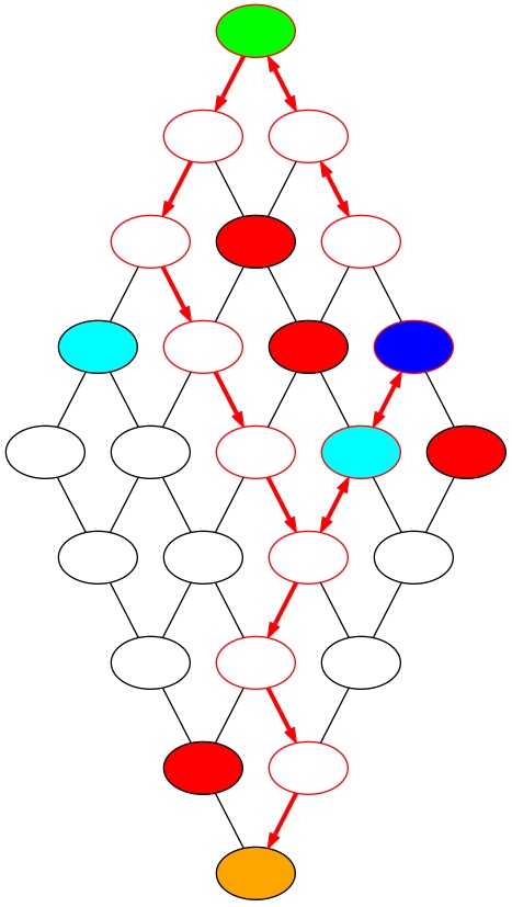
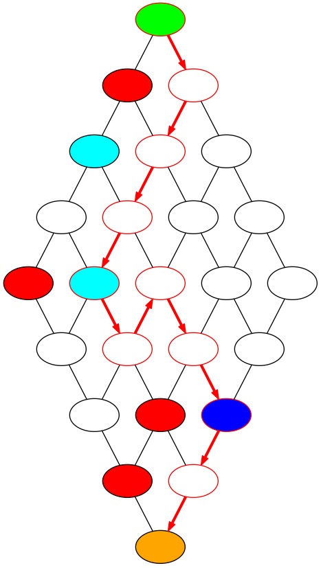
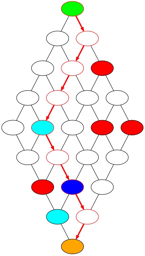
(a)	(b)	(c)

Figure 1: Three sample paths produced by our receding horizon algorithm to solve the scLTL-constrained informative path planning problem. The red transitions indicate the path followed by the robot with arrows indicating direction. The specification is “Beginning at green, visit a light blue region, and then visit a dark blue region, and finally visit the orange region while always avoiding red regions”. This corresponds to the formula in (14) where the orange state is ‘C’, red states are ‘U’, light blue are ‘D1’, and dark blue are ‘D2’.

In order to compare the performance of Algorithms 1 and 2, we solved (14) over a single 6 x 6 transition system generated in the same manner as above. We chose the larger system in order to make comparisons over a larger number of accepting runs. We used Algorithm 1 to find the optimal path in the constrained environment and constructed the pmf of the terminal entropy. We also performed 250 Monte Carlo trials using Algorithm 2 over the same environment and constructed the empirical pmf of the resulting terminal entropies. Histogram representations of the two pmfs are shown in Figure 2. The mean, median, and variance are 26.30 bits, 26.44 bits, and 3.67 $\text{bits}^{2}$, respectively, for the pmf from Algorithm 1 and 25.86 bits, 26.44 bits, and 2.80 $\text{bits}^{2}$, respectively, for the empirical pmf from Algorithm 2. These results confirm our intuition about reactivity and performance: Algorithm 2 performs better in expectation and has lower performance variability than Algorithm 1.

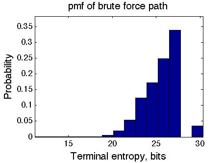
(a)

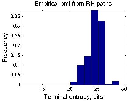
(b)

Figure 2: Histograms of (a) the pmf of the terminal entropy found when following the path from Algorithm 1 and (b) the empirical pmf of the terminal entropy that resulted when the paths were calculated using Algorithm 2. These histograms show that the mean and variance of the pmf of the terminal entropy is lower for the paths generated by Algorithm 2 than the for the path generated by Algorithm 1. The lower mean indicates that using Algorithm 2 will result in a lower entropy estimate on average. The lower variability means that we are less likely to have a high entropy estimate when using Algorithm 2. Algorithm 1 took 1741 s of CPU time to complete and Algorithm 2 took an average of 2.94 s of CPU time per execution to complete.

VI Conclusions and Future Work

In this paper, we considered planning an informative path for a robotic agent subject to temporal logic specifications. We modeled the robot as moving deterministically on a graph with noisy sensor measurements at each node. We proposed a receding horizon algorithm for solving this problem in an on-line, computationally efficient manner while still ensuring specification satisfaction. We compared the performance of our algorithm with an off-line exhaustive search method in a simulation study. Our algorithm out performed the exhaustive search method, producing lower entropy estimates with less computational overhead.

One natural extension to this work is to plan a path that optimizes some other quantity (e.g. path length or graph distance) subject to a minimum level of mutual information. That is, we make the information content of the path a constraint rather than an objective. Another possible extension is to consider cases in which the satisfaction of the temporal logic specification relies on some unknown quantity. Consider, for instance, a rescue robotics scenario in which the robot is tasked not only with finding survivors, but also moving the survivors to a medical station. In this case, planning a path to the medical station is impossible until the robot knows the survivor’s location. This extension would allow us to use formal synthesis methods in a more reactive manner. More generally, we expect that the fusion of information theoretic tools with formal control synthesis will yield robotic control policies that are reactive to noisy, real-world environments while still providing provably correct performance.

References

- [1] Ebru Aydin Gol, Mircea Lazar, and Calin Belta. Language-guided controller synthesis for discrete-time linear systems. In Proceedings of the 15th ACM international conference on Hybrid Systems: Computation and Control, pages 95–104, New York, NY, USA, 2012.
- [2] Christel Baier and Joost-Pieter Katoen. Principles of Model Checking (Representation and Mind Series). The MIT Press, 2008.
- [3] A. Bhatia, L.E. Kavraki, and M.Y. Vardi. Motion planning with hybrid dynamics and temporal goals. In Decision and Control (CDC), 2010 49th IEEE Conference on, pages 1108 –1115, Dec. 2010.
- [4] J. Binney, A. Krause, and G.S. Sukhatme. Informative path planning for an autonomous underwater vehicle. In Robotics and Automation (ICRA), 2010 IEEE International Conference on, pages 4791 –4796, May 2010.
- [5] F. Bourgault, A.A. Makarenko, S.B. Williams, B. Grocholsky, and H.F. Durrant-Whyte. Information based adaptive robotic exploration. In Intelligent Robots and Systems, 2002. IEEE/RSJ International Conference on, volume 1, pages 540 – 545 vol.1, 2002.
- [6] Thomas M. Cover and Joy A. Thomas. Elements of Information Theory. Wiley-Interscience, 2nd edition, 2006.
- [7] Xu Chu Ding, Mircea Lazar, and Calin Belta. Receding horizon temporal logic control for finite deterministic systems. In American Control Conference (ACC), Montreal, Canada, 2012.
- [8] Seng Keat Gan, R. Fitch, and S. Sukkarieh. Real-time decentralized search with inter-agent collision avoidance. In Robotics and Automation (ICRA), 2012 IEEE International Conference on, pages 504 –510, May 2012.
- [9] Aric A. Hagberg, Daniel A. Schult, and Pieter J. Swart. Exploring network structure, dynamics, and function using NetworkX. In Proceedings of the 7th Python in Science Conference (SciPy2008), pages 11–15, Pasadena, CA USA, Aug 2008.
- [10] Leslie Pack Kaelbling and Tomás Lozano-Pérez. Hierarchical task and motion planning in the now. In Robotics and Automation (ICRA), 2011 IEEE International Conference on, pages 1470–1477, 2011.
- [11] Andreas Krause, Carlos Guestrin, Anupam Gupta, and Jon Kleinberg. Near-optimal sensor placements: maximizing information while minimizing communication cost. In Proceedings of the 5th international conference on Information processing in sensor networks, pages 2–10, New York, NY, USA, 2006.
- [12] Orna Kupferman and Moshe Y. Vardi. Model checking of safety properties. Formal Methods in System Design, 2001. volume 19, pages 291-314.
- [13] Timo Latvala. Efficient model checking of safety properties. In Thomas Ball and Sriram Rajamani, editors, Model Checking Software, volume 2648 of Lecture Notes in Computer Science, pages 624–636. Springer Berlin / Heidelberg, 2003.
- [14] D.Q. Mayne, J.B. Rawlings, C.V. Rao, and P.O.M. Scokaert. Constrained model predictive control: Stability and optimality. Automatica, 36, pages 789-814, 1999.
- [15] S. Meguerdichian, F. Koushanfar, M. Potkonjak, and M.B. Srivastava. Coverage problems in wireless ad-hoc sensor networks. In INFOCOM 2001. Twentieth Annual Joint Conference of the IEEE Computer and Communications Societies., volume 3, pages 1380 –1387, 2001.
- [16] Alexandra Meliou, Andreas Krause, Carlos Guestrin, and Joseph M. Hellerstein. Nonmyopic informative path planning in spatio-temporal models. In Proceedings of the 22nd national conference on Artificial intelligence, volume 1, pages 602–607, 2007.
- [17] S. Joe Qin and Thomas A. Badgwell. A survey of model predictive control technology. Control Engineering Practice, 11, pages 733-764, 2003.
- [18] M. Schwager, P. Dames, D. Rus, and V. Kumar. A multi-robot control policy for information gathering in the presence of unknown hazards. In Proceedings of the International Symposium on Robotics Research (ISRR 11), Aug. 2011.
- [19] C. E. Shannon. A mathematical theory of communication. Bell System Technical Journal, 27, pages 379-423,623-656, 1948.
- [20] Amarjeet Singh, Andreas Krause, Carlos Guestrin, William Kaiser, and Maxim Batalin. Efficient planning of informative paths for multiple robots. In Proceedings of the 20th international joint conference on Artifical intelligence, pages 2204–2211, 2007.
- [21] Amarjeet Singh, Andreas Krause, Carlos Guestrin, and William J. Kaiser. Efficient informative sensing using multiple robots. J. Artificial Intelligence Research, 34, pages 707-755, Apr 2009.
- [22] Sebastian Thrun. Simultaneous localization and mapping. In Margaret Jefferies and Wai-Kiang Yeap, editors, Robotics and Cognitive Approaches to Spatial Mapping, volume 38 of Springer Tracts in Advanced Robotics, pages 13–41. Springer Berlin / Heidelberg, 2008.
- [23] Tichakorn Wongpiromsarn, Ufuk Topcu, and Richard Murray. Receding horizon control for temporal logic specifications. In HSCC10: Proceedings of the 13th ACM International Conference on Hybrid Systems:Computation and Control, pages 101–110, 2010.