On Quality of Monitoring for Multi-channel Wireless Infrastructure Networks

Abstract

Passive monitoring utilizing distributed wireless sniffers is an effective technique to monitor activities in wireless infrastructure networks for fault diagnosis, resource management and critical path analysis. In this paper, we introduce a quality of monitoring (QoM) metric defined by the expected number of active users monitored, and investigate the problem of maximizing QoM by judiciously assigning sniffers to channels based on the knowledge of user activities in a multi-channel wireless network. Two types of capture models are considered. The user-centric model assumes frame-level capturing capability of sniffers such that the activities of different users can be distinguished while the sniffer-centric model only utilizes the binary channel information (active or not) at a sniffer. For the user-centric model, we show that the implied optimization problem is NP-hard, but a constant approximation ratio can be attained via polynomial complexity algorithms. For the sniffer-centric model, we devise stochastic inference schemes to transform the problem into the user-centric domain, where we are able to apply our polynomial approximation algorithms. The effectiveness of our proposed schemes and algorithms is further evaluated using both synthetic data as well as real-world traces from an operational WLAN.

1 Introduction

Deployment and management of wireless infrastructure networks (WiFi, WiMax, wireless mesh networks) are often hampered by the poor visibility of PHY and MAC characteristics, and complex interactions at various layers of the protocol stacks both within a managed network and across multiple administrative domains. In addition, today’s wireless usage spans a diverse set of QoS requirements from best-effort data services, to VOIP and streaming applications. The task of managing the wireless infrastructure is made more difficult due to the additional constraints posed by QoS sensitive services. Monitoring the detailed characteristics of an operational wireless network is critical to many system administrative tasks including, fault diagnosis, resource management, and critical path analysis for infrastructure upgrades.

Passive monitoring is a technique where a dedicated set of hardware devices called sniffers, or monitors, are used to monitor activities in wireless networks. These devices capture transmissions of wireless devices or activities of interference sources in their vicinity and store the information in trace files, which can be analyzed distributively or at a central location. Wireless monitoring [1, 2, 3, 4, 5] has been shown to complement wire side monitoring using SNMP and basestation logs since it reveals detailed PHY (e.g., signal strength, spectrum density) and MAC behaviors (e.g, collision, retransmissions), as well as timing information (e.g., backoff time), which are often essential for wireless diagnosis. The architecture of a canonical monitoring system consists of three components: 1) sniffer hardware, 2) sniffer coordination and data collection, and 3) data processing and mining.

Depending on the type of networks being monitored and hardware capability, sniffers may have access to different levels of information. For instance, spectrum analyzers can provide detailed time- and frequency- domain information. However, due to the limit of bandwidth or lack of hardware/software support, it may not be able to decode the captured signal to obtain frame level information on the fly. Commercial-off-the-shelf network interfaces such as WiFi cards on the other hand, can only provide frame level information. The volume of raw traces in both cases tends to be quite large. For example, in the study of the UH campus WLAN, 4 million MAC frames have been collected per sniffer per channel over an 80-minute period resulting in a total of 8 million distinct frames from four sniffers. Furthermore, due to the propagation characteristics of wireless signals, a single sniffer can only observe activities within its vicinity. Observations of sniffers within close proximity over the same frequency band tend to be highly correlated. Therefore, two pertinent issues need to be addressed in the design of passive monitoring systems: 1) what to monitor, and 2) how to coordinate the sniffers to maximize the amount of captured information.

This paper assumes a generic architecture of passive monitoring systems for wireless infrastructure networks, which operate over a set of contiguous or non-contiguous channels or bands. To address the first question, we consider two categories of capturing models differed by their information capturing capability. The first category, called the user-centric model, assumes availability of frame-level information such that activities of different users can be distinguished. The second category is the sniffer-centric model which only assumes binary information regarding channel activities, i.e., whether some user is active in a specific channel near a sniffer. Clearly, the latter imposes minimum hardware requirements, and incurs minimum cost for transferring and storing traces. In some cases, due to hardware constraints (e.g., in wide-band cognitive radio networks) or security/privacy considerations, decoding of frames to extract user level information is infeasible and thus only binary sniffer information might be available for surveillance purpose. We further characterize theoretically the relationship between the two models.

Ideally, a network administrator would want to perform network monitoring on all channels simultaneously. However, multi-radio sniffers are known to be large and expensive to deploy [6]. We therefore assume sniffers in our system are low-cost devices which can only observe one single wireless channel at a time. To maximize the amount of captured information, we introduce a quality-of-monitoring (QoM) metric defined as the total expected number of active users detected, where a user is said to be active at time $t$, if it transmits over one of the wireless channels. The basic problem underlying all of our models can be cast as finding an assignment of sniffers to channels so as to maximize the QoM. QoM is an important metric that quantifies the efficiency of monitoring solutions to systems where it is important to capture as comprehensive information as possible (e.g.: intrusion/anomaly detection [7, 8] and diagnosing systems [9, 10]).

We note that the problem of sniffer assignment, in an attempt to maximize the QoM metric, is further complicated by the dynamics of real-life systems such as: 1) the user population changes over time (churn), 2) activities of a single user is dynamic, and 3) connectivity between users and sniffers may vary due to changes in channel conditions or mobility. These practical considerations reveal the fundamental intertwining of “learning”, where the usage pattern of wireless resources is to be estimated online based on captured information, and “decision making”, where sniffer assignments are made based on available knowledge of the usage pattern. In fact, in our earlier work [11], we prove that during learning, each instance of the decision making is equivalent to solving an instance of the sniffer assignment problem with the parameters properly chosen. Thus, effective and efficient algorithms for the sniffer assignment problem is critical. In this paper, we focus on designing algorithms that aim at maximizing the QoM metric with different granularities of a priori knowledge. The usage patterns are assumed to be stationary during the decision period.

Our Contribution

In this paper, we make the following contributions toward the design of passive monitoring systems for multi-channel wireless infrastructure networks

• We provide a formal model for evaluating the quality of monitoring.

• We study two categories of monitoring models that differ in the information capturing capability of passive monitoring systems. For each of these models we provide algorithms and methods that optimize the quality of monitoring.

• We unravel interactions between the two monitoring models by devising two methods to convert the sniffer-centric model to the user-centric domain by exploiting the stochastic properties of underlying user processes.

More specifically, we show that in both the user- and sniffer-centric models considered, a pure strategy where a sniffer is assigned to a single channel suffices in order to maximize the QoM. In the user-centric model, we show that our problem can be formulated as a covering problem. The problem is proven to be NP-hard, and constant-approximation polynomial algorithms are provided. With the sniffer-centric model, we show that although the only information retrieved by the sniffers is binary (in terms of channel activity), the “structure” of the underlying processes is retained and can be recovered. Two different approaches are proposed that utilize the notion of Independent Component Analysis (ICA) [12] and allow mapping the sniffer assignment problem to the user-centric model. The first approach, Quantized Linear ICA (qlICA), estimates the hidden structure by applying a quantization process on the outcome of the traditional ICA, while the second approach, Binary ICA (bICA) [13], decomposes the observation data into OR mixtures of hidden components and recovers the underlying structure. Finally, an extensive evaluation study is carried out using both synthetic data as well as real-world traces from an operational WLAN.

The paper is organized as follows. An overview of related work is provided in Section 2. In Section 3, we formally introduce the QoM metric and the user-centric and sniffer-centric models for a passive monitoring system. The NP-hardness and polynomial-time algorithms for the maximum effort coverage problem that underlies two variants of the user-centric model are discussed in Section 4. The relationship between the user-centric and sniffer-centric models is established in Section 5, where we also describe two schemes for solving the QoM problem under the sniffer-centric model. We present the results of the evaluation study using both synthetic and real traces in Section 6. We discuss issues regarding practical system implementation in Section 7 and finally conclude the paper in Section 8.

2 Related Work

In this section, we provide an overview of related work pertaining to wireless network monitoring, and binary independent component analysis.

Wireless monitoring

There has been much work done on wireless monitoring from a system-level approach, in an attempt to design complete systems, and address the interactions among the components of such systems. The work in [14, 15] uses AP, SNMP logs, and wired side traces to analyze WiFi traffic characteristics. Passive monitoring using multiple sniffers was first introduced by Yeo et al. in [1, 2], where the authors articulate the advantages and challenges posed by passive measurement techniques, and discuss a system for performing wireless monitoring with the help of multiple sniffers, which is based on synchronization and merging of the traces via broadcast beacon messages. The results obtained for these systems are mostly experimental. Rodrig et al. in [3] used sniffers to capture wireless data, and analyze the performance characteristics of an 802.11 WiFi network. One key contribution was the introduction of a finite state machine to infer missing frames. The Jigsaw system, that was proposed in [4], focuses on large scale monitoring using over 150 sniffers.

A number of recent works focused on the diagnosis of wireless networks to determine causes of errors. In [16], Chandra et al. proposed WiFiProfiler, a diagnostic tool that utilizes exchange of information among wireless hosts about their network settings, and the health of network connectivity. Such shared information allows inference of the root causes of connectivity problems. Building on their monitoring infrastructure, Jigsaw, Cheng et al. [17] developed a set of techniques for automatic characterization of outages and service degradation. They showed how sources of delay at multiple layers (physical through transport) can be reconstructed by using a combination of measurements, inference and modeling. Qiu et al. in [18] proposed a simulation based approach to determine sources of faults in wireless mesh networks caused by packet dropping, link congestion, external noise, and MAC misbehavior.

All the afore-mentioned work focuses on building monitoring infrastructure, and developing diagnosis techniques for wireless networks. The question of optimally allocating monitoring resources to maximize captured information remains largely untouched. In [19], Shin and Bagchi consider the selection of monitoring nodes and their associated channels for monitoring wireless mesh networks. The optimal monitoring is formulated as maximum coverage problem with group budget constraints (denoted MC-GBC), which was previously studied by Chekuri and Kumar in [20]. The user-centric model results in a problem formulation that is similar to (albeit different from) the one addressed in [19]. On one hand, we assume all sniffers may be used for monitoring (hence parting with our problem being akin to the classical maximum-coverage problem, while on the other hand we focus on the weighted version of the problem, where elements to be covered have weights. One should note that all the lower bounds mentioned in [20, 19] do not apply to our problem.

Binary independent component analysis

Binary ICA is a special variant of the traditional ICA, where linear mixing of continuous signals is assumed. In binary ICA, boolean mixing (e.g., OR, XOR etc.) of binary signals is considered. Existing solutions to binary ICA mainly differ in their assumptions of prior distribution of the mixing matrix, noise model, and/or hidden causes. In [21], Yeredor considers binary ICA in XOR mixtures and investigates the identifiability problem. A deflation algorithm is proposed for source separation based on entropy minimization. In [21] the number of independent random sources $K$ is assumed to be known. Furthermore, the mixing matrix is a $K$-by-$K$ invertible matrix. In [22], an infinite number of hidden causes following the same Bernoulli distribution is assumed. Reversible jump Markov chain Monte Carlo and Gibbs sampler techniques are applied. In contrast, in our model, the hidden causes may follow different distributions. Streith et al. [23] study the problem of multi-assignment clustering for boolean data, where an object is represented by a boolean attribute vector. The key assumption made in this work is that elements of the observation matrix are conditionally independent given the model parameters. This greatly reduces the computational complexity and makes the scheme amenable to gradient descent optimization solution; however, the assumption is in general invalid. In [24], the problem of factorization and de-noising of binary data due to independent continuous sources is considered. The sources are assumed to be following a beta distribution and not binary. Finally, [22] considers the under-represented case of less sensors than sources with continuous noise, while [24, 23] deal with the over-determined case, where the number of sensors is much larger than the number of sources.

3 Problem formulation

3.1 Notation and network model

Consider a system of $m$ sniffers, and $n$ users, where each user $u$ operates in one of $K$ channels, $c(u)\in{\cal K}=\left\{1,\ldots,K\right\}$. The users can be wireless (mesh) routers, access points or mobile users. At any point in time, a sniffer can only monitor packet transmissions over a single channel. We assume the propagation characteristics of all channels are similar. We represent the relationship between users and sniffers using an undirected bi-partite graph $\mathcal{G}=(S,U,E)$, where $S$ is the set of sniffer nodes and $U$ is the set of users. Note that $\mathcal{G}$ represents a general relationship between the users and sniffers, and no propagation or coverage model is assumed. An edge $e=(s,u)\in E$ exists between sniffer $s\in S$ and user $u\in U$ if $s$ can capture the transmission from $u$, or equivalently, $u$ is within the monitoring range of $s$. If transmissions from a user cannot be captured by any sniffer, the user is excluded from $\mathcal{G}$. For every vertex $v\in U\cup S$, we let $N(v)$ denote vertex $v$’s neighbors in $\mathcal{G}$. For users, their neighbors are sniffers, and vice versa. We will also refer to $G$ as the binary $m\times n$ adjacency matrix of graph $\mathcal{G}$.

We will consider sniffer assignments of sniffers to channels, $a:S\rightarrow{\cal K}$. Given a sniffer assignment $a$, we consider a partitioning of the set of sniffers $S=\bigcup_{k=1}^{K}{S_{k}}$, where $S_{k}$ is the set of sniffers assigned to channel $k$. We further consider the corresponding partition of the set of users $U=\bigcup_{k=1}^{K}{U_{k}}$, where $U_{k}$ is the set of users operating in channel $k$. Let $\mathcal{G}_{k}=(S_{k},U_{k},E_{k})$ denote the bipartite subgraph of $\mathcal{G}$ induced by channel $k$. Given any sniffer $s$, we let $N_{k}(s)=N(s)\cap U_{k}$, i.e., the set of neighboring users of $s$ that use channel $k$.

A monitoring strategy determines the channel(s) a sniffer monitors. It could be a pure strategy, i.e., the channel a sniffer is assigned to is fixed, or a mixed strategy where sniffers choose their assigned channel in each slot according to a certain distribution. Formally, let $\mathcal{A}=\left\{a\mid a:S\rightarrow{\cal K}\right\}$ be the set of all possible assignments. Let $\pi:\mathcal{A}\rightarrow[0,1]$ be a probability distribution over the set of sniffer assignments. We refer to such a distribution as a mixed strategy. A pure strategy that selects a single channel per sniffer is a special case of mixed strategies, namely, $\pi(a)=1$. It follows that the pure strategy is generally suboptimal comparing to the mixed strategy. However, as shown in the next section, the optimal solution can be obtained using just a pure strategy.

In this paper we consider the problem of finding the monitoring strategy that maximizes QoM, defined as the expected number of users detected given the sniffer assignments. The main notations used in this paper are summarized in Table I.

TABLE I: Notations

$m,n,$	number of sniffers, users,
$K,T$	channels, and observations
	bi-partite graph representing
$\mathcal{G}$	user and sniffer adjacency
$S$	set of sniffers nodes in $\mathcal{G}$
$U$	set of users in $\mathcal{G}$
$\mathcal{A}$	set of all possible sniffer-channel assignments
	vector of $m$ binary random variables
$\mbox{$\mathbf{x}$}_{m\times 1}$	from $m$ sniffers
	vector of $n$ binary random variables
$\mbox{$\mathbf{y}$}_{n\times 1}$	from $n$ users
$\mbox{\boldmath$X$}_{m\times T}$	collection of $T$ observations of $\mathbf{x}$
$\mbox{\boldmath$Y$}_{n\times T}$	collection of $T$ observations of $\mathbf{y}$
$\mbox{\boldmath$G$}_{m\times n}$	binary adjacency matrix of $\mathcal{G}$
$\mbox{$\mathbf{p}$}_{1\times n}$	active probability vector of $n$ users
$c(u)$	active channel of user $u$
$\mathcal{A}(u)$	sniffer assignments that can monitor user $u$
$\pi(a)$	probability distribution of assignment $a$

3.2 Models for Observing User Access Patterns

In this section, two categories of parametric models are proposed to describe the observability of usage patterns. We assume time is separated into slots, where each slot represents a fixed duration of time. A user is active if there exists a transmission event from the user during the slot time. In the experiments, slot time is chosen to be on the same order of maximum packet transmission time. Furthermore, we assume all channel and users’ statistics remain stationary for the monitoring period of $T$ time slots.

User-centric model

First, we consider transmission events in the network from the user’s viewpoint. We assume that $G$ is known by inspecting the packet header information from each sniffer’s captured traces.

In the user-centric model, the transmission probabilities of the users $\mbox{$\mathbf{p}$}=\{p_{u}|u\in U\}$ are known and assumed to be independent . $p_{u}$ denotes the transmission probability of user $u$. $p_{u}$ and $G$ can be estimated by putting all sniffers in the same channel and iterating through all possible channels for sufficiently long time. Each user process may be IID or non-IID over time.

Consider a wireless network with 2 sniffers and 2 users on 2 channels (Figure 1). User $u_{1}$ and $u_{2}$ are active on channels 1 and 2, respectively. Transmission probabilities of users are $p_{1}=0.2$ and $p_{2}=0.5$. User-centric model assumes $G$ and $\mbox{$\mathbf{p}$}=\{p_{1},p_{2}\}$ are available. Note that the maximum value of QoM in the above network is 0.7 attained when $s_{1}$ and $s_{2}$ are assigned to channels 1 and 2, respectively.

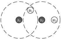
$$\mbox{\boldmath$G$}=\begin{bmatrix}1&0\\ 1&1\\ \end{bmatrix}$$

Figure 1: A toy example. Users are shown in white circles and sniffers are shown in black circles. Sniffer range indicates weather or not a sniffer can capture a user’s transmissions.

Sniffer-centric model

The user-centric model requires detailed knowledge of each user’s activities. This necessitates frame-level capturing capability by the passive monitoring system. In the sniffer-centric model, only binary information (on or off) of the channel activity at each sniffer is observed.

We denote by $\mbox{$\mathbf{x}$}_{k}$ the binary vector of observations when all sniffers operate on channel $k$ and by $\mbox{\boldmath$X$}_{k}$ the collection of $T$ realizations of $\mbox{$\mathbf{x}$}_{k}$. We assume that sniffers observations on different channels are independent. However, dependency exists among observations of sniffers operating in the same channel (as a result of transmissions made by the same set of users). Given an assignment $a$, a complete characterization of the sniffers’ observations is given by the joint probability distribution $\mathcal{P}_{a}(\mbox{$\mathbf{x}$}_{k})$, $k=1,\ldots,K$. Here, $\mathcal{P}_{a}(\mbox{$\mathbf{x}$}_{k})$ is implicitly dependent on the assignment $a$ such that if sniffer $i$ is not assigned to the $k$’th channel, its binary observation $\mbox{$\mathbf{x}$}_{k}(i)$ is always zero. By independence of different channels we have $\mathcal{P}_{a}(\mbox{$\mathbf{x}$})=\prod_{k=1}^{K}{\mathcal{P}_{a}(\mbox{$\mathbf{x}$}_{k})}$.

Consider again the network in Figure 1. Over $T$ time slots, we have two observation matrices $\mbox{\boldmath$X$}_{1}$ and $\mbox{\boldmath$X$}_{2}$ at the same dimension ($2\times T$) corresponding to the activities on two channels. The first and second line in each matrix contain observations from sniffers $s_{1}$ and $s_{2}$, respectively. Sniffer-centric model assumes only the availability of $\mbox{\boldmath$X$}_{1}$ and $\mbox{\boldmath$X$}_{2}$, while $G$ and $\mathbf{p}$ are unknown.

Clearly, the sniffer-centric model is not as expressive as the user-centric model (formally characterized in Section 5.1). However, it has the advantage of being based on aggregated statistics, which are likely to remain stationary in the presence of moderate user-level dynamics, such as joining and leaving the networks, or changes in transmission activities (e.g., busy or thinking time). Furthermore, obtaining such binary information is less costly in both hardware requirements and communication/storage complexity.

4 QoM under the User-Centric Model

Under the user-centric model the goal is to maximize the expected number of active users monitored. Recall that $p_{u}$ is the transmission probability of user $u$. This problem can be formulated formally by:

$$\begin{array}[]{ll}\underset{\pi(a)}{\max}&\sum_{u\in U}{p_{u}\sum_{a\in\mathcal{A}(u)}{\pi(a)}}\\ \mbox{s.t.}&\pi(a)\in[0,1]\\ &\sum_{a\in\mathcal{A}}{\pi(a)}=1,\end{array}$$ (1)

where $\mathcal{A}(u)$ is the set of assignments that monitors user $u$, i.e., $\mathcal{A}(u)=\left\{a\mid\exists s\in N(u)\mbox{ s.t. }a(s)=c(u)\right\}$. The objective function calculates the opportunity for all users to be monitored given the probability of each assignment (QoM). It can be written as,

$$\sum_{a\in\mathcal{A}}{\pi(a)\sum_{u\in U}{p_{u}\cdot{\mathbb{I}}_{\{a\in\mathcal{A}(u)\}}}},$$ (2)

where ${\mathbb{I}}_{\{\cdot\}}$ is an indicator function. From Eq. (2) it is clear that a pure strategy can be adopted and is optimal, i.e., an optimal assignment is given by

$$a^{*}=\arg\max_{a}{\sum_{u\in U}{p_{u}\cdot{\mathbb{I}}_{\{a\in\mathcal{A}(u)\}}}}.$$ (3)

4.1 MAX-EFFORT-COVERAGE problem

Under the user-centric model, the objective to find the sniffer-channel assignment that can monitor the largest (weighted) set of users, subject to the constraint that each sniffer can only monitor one of the $K$ channels at a time. We henceforth refer to the problem as MAX-EFFORT-COVERAGE (MEC) problem. Note that in MEC  the weights can in fact be any non-negative values and are not limited to $[0,1]$. The MEC problem can be cast as the following integer program (IP):

$$\begin{array}[]{rll}\underset{z}{\max}&\sum_{u\in U}p_{u}y_{u}\\[5.69046pt] \mbox{s.t.}&\sum_{k=1}^{K}z_{s,k}\leq 1&\quad\forall s\in S\\ &y_{u}\leq\sum_{s\in N(u)}z_{s,c(u)}&\quad\forall u\in U\\ &y_{u}\leq 1&\quad\forall u\in U\\ &y_{u},z_{s,k}\in\left\{0,1\right\}&\quad\forall u,s,k.\end{array}$$ (4)

Each sniffer is associated with a set of binary decision variables, $z_{s,k}=1$ if the sniffer is assigned to channel $k$; 0, otherwise. $y_{u}$ is a binary variable indicating whether or not user $u$ is monitored, and $p_{u}$ is the weight associated with user $u$. The objective function characterizes the number of (weighted) users that can be monitored with assignment $z$.

One should first note that the problem is trivial if $K=1$, since all sniffers would simply be assigned to the sole available channel. We can therefore assume that $K\geq 2$. The MEC problem can be viewed as a special case of the MC-GBC (mentioned in Section 2), where all sniffers are used. One should note that previous hardness results for MC-GBC (both NP-hardness, as well as hardness of approximation) were based on a reduction to the standard maximum coverage problem. It follows that none of these proofs are applicable to the MEC problem. Surprisingly, there has not been any work done explicitly on the MEC problem, which seems to be a natural and important variant of the maximum coverage problem.

4.2 Hardness of MEC

In what follows we show that the MEC problem is NP-hard for $K\geq 2$, even for the unweighted case (i.e., where $p_{u}=1$ for all $u\in U$). The hardness of the MEC problem actually follows from the choices available to the different sniffers. It is inherently different from the hardness suggested for the MC-GBC problem, which follows from limiting the number of sniffers one is allowed to use. We prove hardness of MEC using a reduction from the problem of Monotone-3SAT (MON3SAT), which is known to be NP-hard (see [27, 28]). In MON3SAT we are given as input an instance of 3SAT where every clause consists of either solely positive variables, or solely negated variables. The goal is to decide whether or not there exists an assignment which satisfies all clauses.

In [29], we proved that the the unweighted MEC problem is NP-hard, even for $K=2$. The result implies that one would have to settle for approximate solutions to MEC. We first note that Guruswami and Khot show in [30] that MON3SAT is NP-hard to approximate within a factor of $7/8+\varepsilon$ for every $\varepsilon>0$. The following is a corollary of the above fact:

Corollary 1

The MEC problem is NP-hard to approximate to within a factor of $7/8+\varepsilon$ for every $\varepsilon>0$.

4.3 Algorithms for MEC

Since MEC is a special case of the MC-GBC problem, we can use the available approximation algorithms for MC-GBC (e.g., [20, 19]) to solve our problem in the user-centric model. In what follows we give a brief overview of the algorithms we use.

The Greedy algorithm

The Greedy algorithm iteratively assigns sniffers to users, where at each step it chooses the sniffer and the assignment that (locally) maximizes the weight of coverage of those not yet monitored users.

It is proven in [20] that in the unweighted case, i.e., where all users have the same weight, Greedy guarantees to produce a $\frac{1}{2}$-approximate solution, and that this is tight. The following theorem shows that the same holds also for the weighted case, which generalizes the MEC problem.

Theorem 2

Greedy is a $\frac{1}{2}$-approximation algorithm for the weighted MC-GBC problem.

LP-based algorithm

This algorithm is based on solving the LP-relaxation of the IP formulation for MEC appearing in (4). Once we have an optimal solution to the LP-relaxation, we round the fractional solution into an integral solution, with e.g., the probabilistic rounding technique of Srinivasan [31]. We next sketch the basic idea of this probabilistic rounding technique. Let $z^{*}$ be an optimal solution to the LP relaxation of (4), and let $s$ be any sniffer. If $\sum_{k}z^{*}_{s,c}>0$, one can view the induced solution $z^{*}_{s}:C\rightarrow[0,1]$ as a probability measure over the different channels (via normalization). The goal is to decide on an integral channel assignment for $s$, namely, setting each $z^{*}_{s,c}$ to a value in $\left\{0,1\right\}$ such that exactly one variable out of the $k$ variables corresponding to sniffer $s$ is set to the value 1. The algorithm builds a binary tree whose leaves corresponds to the $k$ variables $z_{s,k}$ associated with sniffer $s$, and pairs unset variables in a bottom-up fashion. The pairing is made such that an internal node sets at least one of the variables corresponding to its children. This is done while adjusting the (probability) value of the (other) unset variable. This approach is proven to produce a valid assignment in linear time [31]. We refer to the above algorithm as ProbRand.

Theorem 3

ProbRand is a $(1-1/e)$-approximation algorithm for the weighted MC-GBC problem.

We note that the approximation guarantee of the LP-based algorithms are best possible for the MC-GBC problem. However, this lower bound does not necessarily hold for the MEC problem.

5 QoM under the Sniffer-Centric Model

The user-centric model is more expressive than the sniffer-centric model, which assumes the availability of the binary observation matrix $X$ only. However, we will show in this section the two models are intrinsically connected by devising algorithms to infer $G$ and $\mathbf{p}$ from $X$.

Recall that in the sniffer-centric model, given an assignment $a\in\mathcal{A}$, $\prod_{k=1}^{K}{\mathcal{P}_{a}(\mbox{$\mathbf{x}$}_{k})}$ is the probability distribution of binary observations from $m$ sniffers. Let $w(\mbox{$\mathbf{x}$}_{k})$ be the number of active users captured by sniffers in channel $k$ given sniffer observations $\mbox{$\mathbf{x}$}_{k}$. The MEC problem under the sniffer-centric model is defined as follows.

$$\begin{array}[]{ll}\underset{\pi(a)}{\max}&\sum_{a\in\mathcal{A}}{\pi(a)\sum_{k=1}^{K}{{\mathbb{E}}\left[w(\mbox{$\mathbf{x}$}_{k})\right]}}\\ \mbox{s.t.}&\pi(a)\in[0,1]\\ &\sum_{a\in\mathcal{A}}{\pi(a)}=1,\end{array}$$ (5)

The expectation is with respective to $\mathcal{P}_{a}(\mbox{$\mathbf{x}$}_{k})$. QoM in sniffer-centric model can be explained as the expected number of active users captured on all channels given the assignment probabilities. Clearly, a pure strategy suffices, i.e., there exists an optimal assignment such that,

$$a^{*}=\arg\max_{a}\sum_{k=1}^{K}{{\mathbb{E}}\left[w(\mbox{$\mathbf{x}$}_{k})\right]}.$$ (6)

Even with pure strategies, the optimization problem defined in (5) is still challenging to solve directly. The main difficulty arises from the evaluation of ${\mathbb{E}}\left[w(\mbox{$\mathbf{x}$}_{k})\right]$. Given $\mbox{$\mathbf{x}$}_{k}$, one cannot decide how many users are active. Consider two scenarios. In the first case, two users are observed by two sniffers respectively. In the second case, a single user is observed by both sniffers. From binary observations alone, one cannot distinguish the two cases, which correspond to different number of active users. Furthermore, in contrast to the user-centric model, where transmission activities from different users are independent, observations of sniffers are correlated. As a result, $\mathcal{P}_{a}(\mbox{$\mathbf{x}$}_{k})$ cannot be simplified as a product form. This motivates us to exploit the underlying (though not directly observable) independence among users, and map the optimization problem in sniffer-centric model to QoM under the user-centric model.

In the sniffer-centric model, each sniffer only reports binary output regarding the activities in the channel currently monitored by that sniffer, and thus the access probability of the users as well as the bipartite graph $\mathcal{G}$, are both hidden. Recall that $G$ refers to the adjacency binary matrix of $\mathcal{G}$. We first derive the sufficient and necessary conditions for unraveling the transmission probabilities of the users given $G$ and $\mathcal{P}(\mbox{$\mathbf{x}$})$.

Let $\mbox{$\mathbf{y}$}=\left\{y_{1},y_{2},\ldots,y_{n}\right\}^{T}$ be a vector of $n$ binary random variables, where $y_{j}=1$ if user $j$ transmits in its associated channel, and $y_{j}=0$ otherwise. $\mbox{$\mathbf{y}$}_{k}$ is the vector of activities for users transmitting on channel $k$ (i.e., users in $U_{k}$). The joint distribution of $\mathbf{y}$ is given by $\mathcal{P}(\mbox{$\mathbf{y}$})=\prod_{y_{j}=1}p_{j}\prod_{y_{j}=0}(1-p_{j})$. The product form is due to the independence among users’ activities. The main question we aim to answer is: given the vector $\mbox{$\mathbf{x}$}_{k}$ of sniffers’ observations, what knowledge can be obtained regarding $\mbox{$\mathbf{y}$}_{k}$? Throughout this section, unless otherwise specified, we limit the discussion to users and sniffers in a fixed channel $k$, and drop the subscript. We will also denote by $g_{ij}$ the entry in the $i$’th row and $j$’th column of $G$.

Using the adjacency matrix, and using $\wedge$ to represent Boolean AND and $\vee$ to represent Boolean OR, we have the following:

$$x_{i}=\bigvee_{j=1}^{n}{g_{ij}\wedge y_{j}},\mbox{ $i=1,\ldots,m$},$$ (7)

i.e., $x_{i}=1$ iff there exists a user $j$ within the range of sniffer $i$ ($g_{ij}=1$) that transmits ($y_{j}=1$). Define the set $\mbox{\boldmath$Y$}(\mbox{$\mathbf{x}$})=\{\mbox{$\mathbf{y}$}\mid\bigvee_{j=1}^{n}{g_{ij}\wedge y_{j}}=x_{i},\forall i\},$ i.e., the set of user activity profiles that are consistent with the sniffers’ observations. Therefore,

$$\mathcal{P}(\mbox{$\mathbf{x}$})=\mathcal{P}(\mbox{$\mathbf{y}$}\in\mbox{\boldmath$Y$}(\mbox{$\mathbf{x}$}))=\sum_{\mbox{$\mathbf{y}$}\in\mbox{\boldmath$Y$}(\mbox{$\mathbf{x}$})}\mathcal{P}(\mbox{$\mathbf{y}$})$$ (8)

An example network with sniffers and users, the corresponding bipartite graph, and its matrix representation $G$ are given in Figure 2.

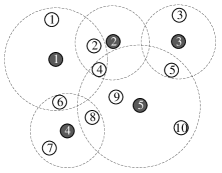
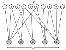
$$\mbox{\boldmath$G$}=\begin{bmatrix}1&\hskip 4.2679pt1&\hskip 4.2679pt0&\hskip 4.2679pt1&\hskip 4.2679pt0&\hskip 4.2679pt1&\hskip 4.2679pt0&\hskip 4.2679pt0&\hskip 4.2679pt0&\hskip 4.2679pt0\\ 0&\hskip 4.2679pt1&\hskip 4.2679pt0&\hskip 4.2679pt1&\hskip 4.2679pt0&\hskip 4.2679pt0&\hskip 4.2679pt0&\hskip 4.2679pt0&\hskip 4.2679pt0&\hskip 4.2679pt0\\ 0&\hskip 4.2679pt0&\hskip 4.2679pt1&\hskip 4.2679pt0&\hskip 4.2679pt1&\hskip 4.2679pt0&\hskip 4.2679pt0&\hskip 4.2679pt0&\hskip 4.2679pt0&\hskip 4.2679pt0\\ 0&\hskip 4.2679pt0&\hskip 4.2679pt0&\hskip 4.2679pt0&\hskip 4.2679pt0&\hskip 4.2679pt1&\hskip 4.2679pt1&\hskip 4.2679pt1&\hskip 4.2679pt0&\hskip 4.2679pt0\\ 0&\hskip 4.2679pt0&\hskip 4.2679pt0&\hskip 4.2679pt1&\hskip 4.2679pt1&\hskip 4.2679pt0&\hskip 4.2679pt0&\hskip 4.2679pt1&\hskip 4.2679pt1&\hskip 4.2679pt1\end{bmatrix}\begin{matrix}x_{1}\\ x_{2}\\ x_{3}\\ x_{4}\\ x_{5}\end{matrix}\vspace{-2mm}$$

$$\hskip 14.22636pt\begin{matrix}y_{1}&y_{2}&y_{3}&y_{4}&y_{5}&y_{6}&y_{7}&y_{8}&y_{9}&y_{10}\end{matrix}$$

Figure 2: A sample network scenario with number of sniffers $m=5$, number of users $n=10$, its bipartite graph transformation and its matrix representation. White circles represent independent users, black circles represent sniffers and dashed lines illustrate sniffers’ coverage range.

5.1 Relationship between the user-centric and sniffer-centric models with known $G$ and unknown $\mathbf{p}$

The necessary and sufficient conditions that uniquely determine $\mathbf{p}$ using $G$ and $\mathcal{P}(\mbox{$\mathbf{x}$})$ is characterized in the following theorem.

Theorem 4

Given $\mathcal{G}=(S,U,E)$, $\mathbf{p}$ can be uniquely determined by $\mathcal{P}(\mbox{$\mathbf{x}$})$ iff $\forall u_{j}\neq u_{j^{\prime}}\in U$, $N(u_{j})\neq N(u_{j^{\prime}})$.

Proof:

• It is easy to see that the necessary condition holds. If two users have the same set of sniffer neighbors, unless packet headers are analyzed, their activities cannot be distinguished.

• To prove the sufficient condition, we construct a procedure to determine $\mathbf{p}$ from sniffer’s joint distribution $\mathcal{P}(\mbox{$\mathbf{x}$})$.

  Case 1: First, we consider a more restrictive constraint, namely, $\forall u_{j}\neq u_{j^{\prime}}\in U$, $N(u_{j})\not\subseteq N(u_{j^{\prime}})$. We let $g_{j}$ denote the $j$’th column of the adjacency matrix $G$, i.e., a binary vector of length $m$. In other words, $g_{j}$ is the coverage vector of the $j$’th sniffer. Since $\forall u_{j}\neq u_{j^{\prime}}\in U$, $N(u_{j})\not\subseteq N(u_{j^{\prime}})$, we have $g_{j}\cup g_{j^{\prime}}\neq g_{j}$ and $g_{j}\cup g_{j^{\prime}}\neq g_{j^{\prime}}$. From (8), we have

  $$\mathcal{P}(\mbox{$\mathbf{x}$}=g_{j})=p_{j}\prod_{j^{\prime}\in U,j^{\prime}\neq j}{(1-p_{j^{\prime}})},$$

  Since $\mathcal{P}(\mbox{$\mathbf{x}$}=\emptyset)=\prod_{j\in U}{(1-p_{j})}$ (recall by our abuse of notation that $\emptyset$ is the all-zero vector of length $m$), we have

  $$p_{j}=\frac{\mathcal{P}(\mbox{$\mathbf{x}$}=g_{j})}{\mathcal{P}(\mbox{$\mathbf{x}$}=g_{j})+\mathcal{P}(\mbox{$\mathbf{x}$}=\emptyset)}.$$ (9)

  Case 2: Now we consider the case when the condition $\forall u_{j}\neq u_{j^{\prime}}\in U$, $N(u_{j})\not\subseteq N(u_{j^{\prime}})$ is violated. Without loss of generality, assume only one such pair $(j,j^{\prime})$ exist and $N(u_{j^{\prime}})\subseteq N(u_{j})$ (analysis for more complicated cases follows the same line of arguments). In this case, $p_{j^{\prime}}$ can be derived as in the previous case. However, equation (9) does not hold for user $j$ any more since if $\mbox{$\mathbf{x}$}=g_{j}$, user $j^{\prime}$ may or may not be active. More specifically,

  $$\mathcal{P}(\mbox{$\mathbf{x}$}=g_{j})=p_{j}\prod_{j^{\prime\prime}\in U,j^{\prime\prime}\neq j,j^{\prime}}{(1-p_{j^{\prime\prime}})}.$$ (10)

  Therefore, we have

  $$p_{j}=\frac{\mathcal{P}(\mbox{$\mathbf{x}$}=g_{j})(1-p_{j^{\prime}})}{\mathcal{P}(\mbox{$\mathbf{x}$}=g_{j})(1-p_{j^{\prime}})+\mathcal{P}(\mbox{$\mathbf{x}$}=\emptyset)}.$$ (11)

  In other words, the active probability of users can be computed by considering the users with the smallest degree in $G$ first, and then applying (11) iteratively in ascending order of node degree.

∎

The above theorem essentially shows that in the sniffer-centric model, if $G$ is known, then one can effectively determine the transmission probabilities of the users. In presence of measurement noise, methods such as Expectation-Maximization can be applied. We therefore obtain an instance of the problem corresponding to our user-centric model, which can be solved efficiently using the algorithms described in Section 4.3.

Comment

Though Theorem 4 requires the users be connected to different sets of sniffers, violation of the condition would not affect the channel assignment. For example, when two users $u$ and $v$ are connected to the same set of sniffers, and are thus “indistinguishable” in the binary sniffer observations, we can effectively view them as a single user with active probability $1-(1-p_{u})(1-p_{v})$ if users are active independently, or $p_{u}+p_{v}$ if only one user can be active at a time (e.g., due to CSMA).

5.2 Inference of unknown $G$ and $\mathbf{p}$ using binary ICA

(a) Quantized Linear ICA

(b) Binary ICA

Figure 3: Channel selection algorithm under qlICA and bICA models

In this section, we derive methods to estimate the unknown mixing matrix $G$ and the active probability vector $\mathbf{p}$. Consider again the example in Figure 1. Let sniffers $s_{1}$ and $s_{2}$ be assigned to channel 1 and observe the activity of a single user $y_{1}$. In this case, $x_{1}=x_{2}$. Therefore,

$$\begin{array}[]{lll}\mathcal{P}(\mbox{$\mathbf{x}$})&=&\mathcal{P}(x_{1}){\mathbb{I}}_{\{x_{1}=x_{2}\}}\\ &=&\mathcal{P}(y_{1}=x_{1})\\ &=&\left\{\begin{array}[]{ll}p_{1},&x_{1}=1\\ 1-p_{1},&x_{1}=0\end{array}\right..\end{array}$$

Therefore, if the joint distribution of $\mbox{$\mathbf{x}$}_{k}$ is the product of a marginal distribution with an indicator function, and the two marginal distributions are identical, we can infer that both sniffers observe the same set of users. Generally, the joint distribution of $\mathbf{x}$ preserves a certain stochastic “structure” of the user’s activities. We will formalize this observation in the subsequent section by devising two inference methods to estimate $G$ and $\mathbf{p}$ from $\mathcal{P}(\mbox{$\mathbf{x}$})$.

5.2.1 Quantized Linear ICA (qlICA)

First we will estimate $G$ by applying the classic ICA on the binary data followed by a quantization process. Then $\mathcal{P}{(\mbox{$\mathbf{y}$})}$ can then be calculated by solving a quadratic programming problem.

Estimation of $G$

The problem is similar to what was addressed by the Independent Component Analysis (ICA) scheme [12], where the observed data is expressed as a linear transformation of latent variables that are non-Gaussian and mutually independent. Classic ICA assumes that both $\mathbf{y}$ and $\mathbf{x}$ are continuous random variables and that $\mathbf{x}$ is the outcome of a linear mixing of $\mathbf{y}$, and thus is not directly applicable to our problem. We adopt the algorithm presented in [32] with some modifications. The basic idea is as follows.

We first observe that (7) can be simplified using linear mixing and a (coordinate-wise) unit step function.

$$\mbox{$\mathbf{x}$}=\mathbb{U}(\mbox{\boldmath$G$}\mbox{$\mathbf{y}$}),$$ (12)

where $\mathbb{U}(\cdot)$ is a unit step function defined by $\mathbb{U}(r)={\mathbb{I}}_{\{r>0\}}$. By applying the standard ICA on $\mathbf{x}$, we can “decompose” the observation to $\mbox{$\mathbf{x}$}\approx\mbox{\boldmath$L$}\mbox{$\mathbf{s}$}$, with $L$ is the linear mixing matrix and $\mathbf{s}$ is the collection of random sources. However, both $L$ and $\mathbf{s}$ are not the solutions to our problem since they contain fractional values. Therefore, we quantize $L$ to get the inferred binary mixing matrix $\hat{\mbox{\boldmath$G$}}$ as follow,

$$\hat{\mbox{\boldmath$G$}}=\mathbb{U}(\mbox{\boldmath$L$}\Lambda^{-1}-\mbox{\boldmath$T$}).$$ (13)

$\Lambda$ is the diagonal scaling matrix with $\lambda_{ii}=\operatorname{maxstep}(\ell_{i})$, where $\ell_{i}$ is the $i$’th column of $L$, and

$$\operatorname{maxstep}(\mbox{\boldmath$r$})=\left\{\begin{array}[]{ll}\max(\mbox{\boldmath$r$})&\quad\mbox{if }|\max(\mbox{\boldmath$r$})|>|\min(\mbox{\boldmath$r$})|\\ \min(\mbox{\boldmath$r$})&\quad\mbox{otherwise.}\end{array}\right.$$ (14)

$\Lambda$ scales the elements in the mixing matrix to the maximum value 1. The matrix $T$ contains thresholds, such that the higher the threshold value, the sparser $\hat{\mbox{\boldmath$G$}}$ is.

Estimation of $\mathcal{P}{(\mbox{$\mathbf{y}$})}$

Once $\hat{\mbox{\boldmath$G$}}$ is determined, $\mathcal{P}{(\mbox{$\mathbf{y}$})}$ needs to be estimated. From $x_{i}=U(\hat{g}_{i}y_{i})$, where $\hat{g}_{i}$ is the $i$’th row of $\hat{\mbox{\boldmath$G$}}$ (i.e., the estimated coverage vector of sniffer $s_{i}$), we have,

$$p(x_{i}=0)=\prod_{\hat{g}_{ij}=1}{p(y_{j}=0)}.$$ (15)

The product is due to the independence of $y_{i}$’s. Taking $\log(\cdot)$ on both sides, we have

$$\log(p(x_{i}=0))=\sum_{\hat{g}_{ij}=1}{\log(p(y_{j}=0))}.$$ (16)

Let $\alpha_{i}=\log(p(x_{i}=0))$, and $\beta_{i}=\log(p(y_{j}=0))$. Define $\mathbf{\alpha}=\{\alpha_{1},\alpha_{2},\ldots,\alpha_{m}\}^{T}$, and $\mathbf{\beta}=\{\beta_{1},\beta_{2},\ldots,\beta_{n}\}^{T}$. We can calculate $p(y_{j}=0)$ (and consequently obtain $\mathcal{P}{(\mbox{$\mathbf{y}$})}$) by solving the following optimization problem.

$$\begin{array}[]{cc}\underset{\beta}{\min}&\parallel\mathbf{\alpha}-\hat{\mbox{\boldmath$G$}}\mathbf{\beta}\parallel^{2}\\ \mbox{s.t.}&\mathbf{\beta}<0,\end{array}$$ (17)

where $\parallel\cdot\parallel$ is the second norm of a vector. The objective function minimizes the distance between the real observation vector $\mathbf{x}$ and its reconstructed counterpart ($\hat{\mbox{\boldmath$G$}}\beta$). Clearly, this is a constrained quadratic programming problem with a positive semi-definite matrix (i.e., all eigenvalues are non-negative), and can be solved in polynomial time.

Channel selection

With the estimated $\hat{\mbox{$\mathbf{p}$}}$ and $\hat{\mbox{\boldmath$G$}}$ at hand, we effectively transform the sniffer-centric model to the user-centric model. Methods described in Section 4.3 can then be applied to determine the channel assignment of each sniffer.

uantizeICA ~algorithm which infers $\hat{\pp}$ and $\hat{\G}$ is presented in Algorithm~\ref{algo:qlica}
and the complete \qlica\ scheme is illustrated in Figure~\ref{fig:final-algorithm}(a).
%
\begin{algorithm}[h]
\caption{

uantized linear ICA inference QuantizeICA ($X$)
input :  Data matrix $\mbox{\boldmath$X$}_{m\times T}$ init :  $\mbox{\boldmath$T$}=$ threshold matrix 

$\mbox{\boldmath$L$}=$ mixing matrix obtained by applying ICA on $X$ 

$\Lambda=$ diagonal scaling matrix calculated from $L$ 

$\hat{\mbox{\boldmath$G$}}=\mathbb{U}(\mbox{\boldmath$L$}\Lambda^{-1}-\mbox{\boldmath$T$})$ 

Calculate $\alpha$ from $X$ with $\alpha_{i}=\log(p(x_{i}=0))$ 

Obtain $\hat{\mbox{$\mathbf{p}$}}$ by solving the quadratic programming problem in (17) 

output :

$\hat{\mbox{$\mathbf{p}$}}$ and $\hat{\mbox{\boldmath$G$}}$

A toy example

We next give a simple example, which provides insight as to the operations of qlICA. Let us reconsider the network in Figure 1 with $u_{1}$ and $u_{2}$ operate on one single channel. With $T=10$ observations, supposedly we have the activity matrix

$$\mbox{\boldmath$Y$}=\begin{bmatrix}0&0&1&0&0&0&0&0&1&0\\ 0&1&1&0&0&1&1&1&0&0\end{bmatrix}.$$

$y_{ij}=1$ indicates that user $y_{i}$ is active on the channel at time slot $j$. $Y$ is hidden and unknown to us. Since $\mbox{\boldmath$G$}=\begin{bmatrix}1&0\\ 1&1\end{bmatrix}$, we have the observation matrix

$$\mbox{\boldmath$X$}=\begin{bmatrix}0&0&1&0&0&0&0&0&1&0\\ 0&1&1&0&0&1&1&1&1&0\end{bmatrix}.$$

Applying the linear ICA, we obtain

$$\mbox{\boldmath$L$}=\begin{bmatrix}0.30&-0.35\\ -0.20&-0.35\\ \end{bmatrix},\Lambda^{-1}=\begin{bmatrix}-2.89&0\\ 0&-2.89\\ \end{bmatrix}.$$

With threshold $\mbox{\boldmath$T$}=0.5$, solving the equation (13) and the optimization problem (17), we have the following inferred results.

$$\hat{\mbox{\boldmath$G$}}=\begin{bmatrix}0&1\\ 1&1\end{bmatrix},\hat{\mbox{$\mathbf{p}$}}=\{0.5,0.2\}.$$

Inferred results $\hat{\mbox{\boldmath$G$}}$ and $\hat{\mbox{$\mathbf{p}$}}$ are actually permutations of the original mixing matrix $G$ and the active probability $\mathbf{p}$. We see that qlICA can successfully infer information regarding the underlying model from $\mathcal{P}(\mbox{$\mathbf{x}$})$.

5.2.2 Binary ICA (bICA)

Instead of applying a quantization process on the result of linear ICA, we can apply the bICA algorithm proposed in [13] to determine $\mathcal{P}(\mbox{$\mathbf{y}$})$ and $G$ by exploiting the OR mixture model between $\mathbf{y}$ and the observation variable $\mathbf{x}$. Compared with qlICA, bICA explicitly account for the generative model and thus leads to more accurate estimation results. However, this comes at the expense of higher computation complexity. In the worst case, given $m$ sniffers, the run time of the algorithm is $O(m2^{m})$. For completeness, we first define some notation and then outline the bICA algorithms.

Joint estimation of $G$ and $\mathcal{P}(\mbox{$\mathbf{y}$})$

The basic idea of bICA algorithm is as follow: given an observation matrix $X$ from $m$ sniffers, we will first assume that there exists at most $2^{m}$ distinguishable users. Each user is represented in $G$ by a unique column $\in\{0,1\}^{m}$ indicating its connections to $m$ sniffers. $2^{m}$ users are ordered by ascending values of their corresponding columns. We will recursively construct 2 submatrices from $X$ such that the first submatrix captures the joint distribution of activities from the first $2^{m-1}$ users (in product form due to the independence assumption). If the submatrix is small enough, the join distribution can be inferred directly, otherwise, a divide-and-conquer approach is taken. Once the join distribution of the first $2^{m-1}$ users are available, that of the remaining $2^{m-1}$ users can be inferred from the second submatrix. Next, we present in detail the proposed bICA algorithm. Let define $\mbox{\boldmath$X$}_{(h-1)\times T}^{0}$ to be a submatrix of $X$, where the rows correspond to observations of $x_{1},x_{2},\ldots,x_{h-1}$ for $t=1,2,\ldots,T$ such that $x_{ht}=0$, i.e., the first submatrix mentioned above. Also, define $\mbox{\boldmath$X$}_{(h-1)\times T}$ to be the matrix consisting the first $h-1$ rows of $X$, i.e., the second submatrix. Let $\mathcal{F}(.)$ be the frequency function of some event, we have the iterative inference algorithm as illustrated in Algorithm 1.

FindBICA ($X$)

input : Data matrix $\mbox{\boldmath$X$}_{m\times T}$

init : $n=2^{m}-1$;

$\hat{\mbox{$\mathbf{p}$}}$ = $1\times n$ zero vector;

$\hat{\mbox{\boldmath$G$}}$ = $m\times(2^{m}-1)$ matrix with rows corresponding all possible binary vectors of length $m$;

$\varepsilon$ = the minimum threshold for $p_{h}$ to be considered a real component;

21if $m=1$ then $\hat{p_{1}}=\mathcal{F}(x_{1}=0)$;

3 $\hat{p_{2}}=\mathcal{F}(x_{1}=1)$;

54 else if $\mbox{\boldmath$X$}^{0}_{(m-1)\times T}=\emptyset$ then $\hat{p}_{1\ldots 2^{m-1}}$ = FindBICA ($\mbox{\boldmath$X$}_{(m-1)\times T}$);

6 $\hat{p}_{2^{m-1}+1}=1$;

7 $\hat{p}_{2^{m-1}+2\ldots 2^{m}}=0$;

8 else $\hat{p}_{1\ldots 2^{m-1}}$ = FindBICA ($\mbox{\boldmath$X$}^{0}_{(m-1)\times T}$);

9 $\hat{p}^{\prime}_{1\ldots 2^{m-1}}$ = FindBICA ($\mbox{\boldmath$X$}_{(m-1)\times T}$);

1110 for $l=2,\ldots,2^{m-1}$ do $\hat{p}_{l+2^{m-1}}=1-\frac{1-\hat{p}^{\prime}_{l}}{1-\hat{p}_{l}}$;

endfor

12$\hat{p}_{2^{m-1}+1}=\frac{\mathcal{F}{(x_{m}=1\wedge x_{i}=0,\forall i\in[1\ldots m-1])}}{\prod_{l=1\ldots 2^{m}-1,l\neq 2^{m-1}+1}{(1-\hat{p}_{l})}}$;

end if

end if

151413for $h=1,\ldots,2^{m}$ do if $(\hat{p}_{h}<\varepsilon)\vee(\hat{p}_{h}=0)$ then prune $\hat{p}_{h}$ and corresponding column $\hat{g}_{h}$;

end if

endfor

16output : $\hat{\mbox{$\mathbf{p}$}}$ and $\hat{\mbox{\boldmath$G$}}$

Algorithm 1 Incremental binary ICA inference

When the number of observation variables $m=1$, there are only two possible unique sources, one that can be detected by the monitor $x_{1}$, denoted by [1]; and one that cannot, denoted by [0]. Their active probabilities can easily be calculated by counting the frequency of $(x_{1}=1)$ and $(x_{1}=0)$ (lines 1 – 1). If $m\geq 2$, $\mathbf{p}$ and $G$ are estimated through a recursive process. $\mbox{\boldmath$X$}^{0}_{(m-1)\times T}$ is sampled from columns of $X$ that have $x_{m}=0$. If $\mbox{\boldmath$X$}^{0}_{(m-1)\times T}$ is an empty set (which means $x_{mt}=1,\forall t$) then we can associate $x_{m}$ with a constantly active component and set the other components’ probability accordingly (lines 1 – 1). If $\mbox{\boldmath$X$}^{0}_{(m-1)\times T}$ is non-empty, we invoke

indBICA ~on
two sub-matrices $\X^0_{(m-1)\times T}$ and $\X_{(m-1)\times T}$ to determine
$\hat{p}_{1 \ldots 2^{m-1}}$ and $\hat{p}’_{1 \ldots 2^{m-1}}$, then
infer $\hat{p}_{2^{m-1}+1 \ldots 2^{m}}$ (lines~\ref{line4} --
\ref{line8}). 

inally, $\hat{p}_{h}$ and its corresponding column $\hat{g}_{h}$ in $\hat{\mbox{\boldmath$G$}}$ are pruned in the final result if $\hat{p}_{h}<\varepsilon$ (lines 1 – 1).

Channel selection

Now that $\hat{\mbox{$\mathbf{p}$}}$ and $\hat{\mbox{\boldmath$G$}}$ are inferred, we again transform the sniffer-centric model to the user-centric model and apply methods Section 4.3 to find optimal sniffer-channel assignment scenario. The complete bICA scheme is illustrated in Figure 3(b).

A toy example

Again, let us reconsider the network in Figure 1. Recall that $\mbox{$\mathbf{p}$}=\{0.2,0.5\}$, $T=10$ and the observation matrix is

$$\mbox{\boldmath$X$}=\begin{bmatrix}0&0&1&0&0&0&0&0&1&0\\ 0&1&1&0&0&1&1&1&1&0\end{bmatrix}.$$

Following the

indBICA ~algorithm,
we will first decompose $\X$ into $\X^0_{1\times T}$ and $\X_{1\times T}$.
\begin{center}
\vspace{-0.2in}
$$
\X^0_{1\times T} =
\begin{bmatrix}
0&0&0&0
\end{bmatrix},
$$
$$
\X_{1\times T} =
\begin{bmatrix}
0&0&1&0&0&0&0&0&1&0
\end{bmatrix}.
$$
\end{center}

rom $\mbox{\boldmath$X$}^{0}_{1\times T}$, we have $\hat{p}_{0}=1$ and $\hat{p}_{1}=0$. Similarly from $\mbox{\boldmath$X$}_{1\times T}$, we have $\hat{p}^{\prime}_{0}=0.8$ and $\hat{p}^{\prime}_{1}=0.2$. Applying the procedure in Algorithm 1, we have the inferred results:

$$\hat{\mbox{\boldmath$G$}}=\begin{bmatrix}0&1&0&1\\ 0&0&1&1\end{bmatrix},\hat{\mbox{$\mathbf{p}$}}=\{1,0,0.5,0.2\}.$$

The first and second column of $\hat{\mbox{\boldmath$G$}}$ and $\hat{\mbox{$\mathbf{p}$}}$ will be pruned since we are not interested in components that cannot be observed (with $\hat{g}_{i}=0$) or components with their active probabilities smaller than $\varepsilon$ ($\varepsilon$ is set to be 0.01 in this case). Thus yields the final result to be exactly equal to the ground truth. Toy example shows that both qlICA and bICA can accurately predict the underlying model without priory knowledge on the latent variables’ activities in simple cases. The next section will provide an extensive evaluation on performance of qlICA and bICA.

6 Simulation Validation

In this section we evaluate the performance of different algorithms under the user-centric and sniffer-centric models using both synthetic and real traces. Synthetic traces allow us to control the parameter settings while real network traces provide insights on the performance under realistic traffic loads and user distributions. In addition to the Greedy and LP-based algorithm, we also consider Max Sniffer Channel (Max) where a sniffer is assigned to its busiest channel. This scheme is the most intuitive approach in practical networks where the user model is not available and sniffers have to decide their channel assignment non-cooperatively based on local observations. Note it is easy to construct scenarios where Max performs arbitrarily bad. Thus, its worst case performance is unbounded. For the inference scheme in the qlICA model, we used the FastICA algorithm [12] to compute the linear mixing matrix $L$.

6.1 QoM under different models

6.1.1 Synthetic traces

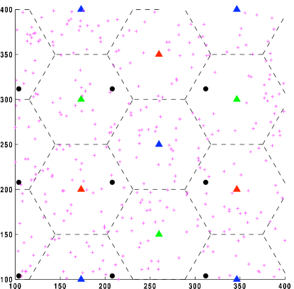
Figure 4: Hexagonal layout with users (‘+’), sniffers (solid dots), base stations (triangles), and channels of each cell (in different triangle colors)

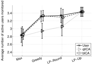
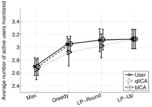
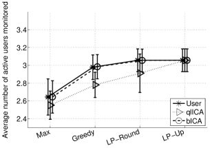
(a) 3 channels	(b) 6 channels	(c) 9 channels

Figure 5: QoM under three models: the user-centric model (User), qlICA and bICA with 3, 6 and 9-channel synthetic traces

In this set of simulations, 500 wireless users are placed randomly in a $500\times 500$ square meter area. The area is partitioned into hexagon cells with circumcircle of radius 86 meters. Each cell is associated with a base station operating in a channel (and so are the users in the cell). The channel to base station assignment ensures that no neighboring cells use the same channel. 25 Sniffers are deployed in a grid formation separated by distance 100 meters, with a coverage radius of $120$ meters. A snap shot of the synthetic deployment is shown in Figure 4. The transmission probability of users is selected uniformly in (0, 0.06], resulting in an average busy probability of 0.2685 in each cell. Threshold $T$ for qlICA is set at 0.5 and threshold $\varepsilon$ for bICA is set at 0.01. We vary the total number of orthogonal channels from 3 to 9. The results shown are the average of 20 runs with different seeds. Figure 5 shows QoM calculated by three algorithms (Max, Greedy and LP-Round) and the theoretical upper bound (LP-Up) on two models using synthetic traces of 3, 6, 9 channels, respectively. Results of the user-centric model are shown in solid lines while results of different inference algorithms (e.g., qlICA and bICA) in the sniffer-centric model are shown in dotted and dashed lines, respectively. In the user-centric model, one can see that the performance of Greedy and the LP-based algorithm with random rounding are comparable to LP-Up, and both outperform Max in all three traces. Recall that according to Max, a sniffer non-cooperatively decides its own channel assignment and selects the most active channel. Clearly, Max does not take into account the correlations among the observations of neighboring sniffers in the same channel. In contrast, in the sniffer centric case, the proposed inference algorithms can indeed extract such a correlative structure from the binary observations as shown by their superior performance over Max. Additionally, we observe that the expected number of users monitored by the algorithms using bICA is higher than that of qlICA and is very close to that attained in the user centric model (where we assumed to have complete knowledge of users’ activities and their relationship to sniffers). This indicates that bICA algorithm indeed produces inferred models that are very close to the ground truths. Having a good estimation of $\hat{\mbox{\boldmath$G$}}$ and $\hat{\mbox{$\mathbf{p}$}}$ as the input, Greedy and LP-Round can produce channel assignments whose performance is close to LP-Up. We further note that by comparing results from Figure 5(a) to Figure 5(c), the QoM metric reduces as the total number of channels increases for all schemes, including LP-Up. This is due to the fact that users scatter over more channels, and a fixed number of sniffers is no longer sufficient to provide good coverage.

6.1.2 Real traces

In this section, we evaluate our proposed schemes using real traces collected from the UH campus wireless network using 21 WiFi sniffers deployed in the Philip G. Hall. Over a period of 6 hours, between 12 p.m. and 6 p.m., each sniffer captured approximately 300,000 MAC frames. Altogether, 655 unique users are observed operating over three channels. The number of users observed on WiFi channels 1, 6, 11 are 382, 118, and 155, respectively. The histogram of user active probability (calculated as the percentage of 20$\mu$s slots that a user is active) is shown in Figure 7. Clearly, most users are active less than 1% of the time except for a few heavy hitters. The average user active probability is 0.0014.

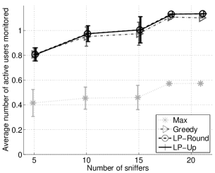
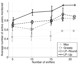
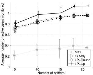
(a) User-centric model	(b) Quantized linear ICA	(c) Binary ICA

Figure 6: QoM under the user-centric and sniffer-centric models with real WiFi traces. In the user-centric model, the results of LP-round coincide with that of the LP-Up. In some cases, the confidence interval is quite small and is thus not observable in the figures.

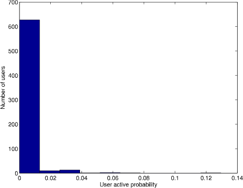
Figure 7: Histogram of user active probability measured as the percentage of active 20$\mu$s slots. The average active probability is 0.0014.

Figure 6 gives the average number of active users monitored under the user-centric model, and under the models inferred by qlICA and bICA. The number of sniffers in the experiments varies from 5 to 21 by including only traces from the corresponding sniffers. The number of channels is fixed at 3. Except for the case with 21 sniffers, all data points are averages of 5 scenarios with different sets of sniffers, chosen uniformly at random. Recall that the average active probability is 0.0014. Thus, for the best channel assignment scenario, the QoM on all channels is around 1. In the user-centric case (Figure 6(a)), both Greedy and LP-Round significantly outperform Max (by around 50%). Moreover, their performance is comparable with LP-Up. As the number of sniffers increases, the average number of users monitored increases but tends to flatten out since most users have been monitored. In the sniffer-centric case, similar trends can be observed when $G$ and $\mathcal{P}(\mbox{$\mathbf{y}$})$ are inferred using qlICA and bICA (Figure 6(b)(c)). bICA outperforms qlICA in general. However, there exists some performance gap in both cases due to the loss of information, when compared with the user-centric model. The real WiFi traces, in contrast to the synthetic scenarios, contain a large number of observations and many “mice” users (users with very low active probability). Most of the time, these users will be removed (since $p_{i}<\varepsilon$), causing higher prediction errors in $\hat{\mbox{\boldmath$G$}}$ and $\hat{\mbox{$\mathbf{p}$}}$.

6.2 Comparison of qlICA and bICA under the sniffer-centric model

To understand the performance difference of qlICA and bICA, in this section, we provide a detailed comparison of the inferred $G$ and $\mathcal{P}(\mbox{$\mathbf{y}$})$ in both schemes.

Performance metrics

We denote by $\hat{\mbox{\boldmath$G$}}$ and $\hat{\mbox{$\mathbf{p}$}}$ the inferred adjacency matrix and the inferred active probability of users, respectively. Two metrics are introduced to measure the accuracy of the inferred quantities.

• Structure Error Ratio. This metric indicates how accurate the adjacency matrix is estimated. It is defined by the Hamming distance between $G$ and $\hat{\mbox{\boldmath$G$}}$ divided by the size of the matrix.

  $$\begin{array}[]{lll}\bar{H}(\mbox{\boldmath$G$},\hat{\mbox{\boldmath$G$}})&\stackrel{{\scriptstyle\Delta}}{{=}}&\frac{1}{mn}\sum_{i=1}^{n}d^{H}(g_{i},\hat{g}_{i})\end{array}$$ (18)

  Due to the possible difference in the number and the order of inferred independent components in $G$ and $\hat{\mbox{\boldmath$G$}}$, we need to perform the structure matching process before estimating $\bar{H}(\mbox{\boldmath$G$},\hat{\mbox{\boldmath$G$}})$. Details of the algorithm can be found in [13].

• Transmission Probability Error. The prediction error in the inferred transmission probability of independent users is measured by the Kullback-Leibler divergence between two probability distributions $\mathbf{p}$ and $\hat{\mbox{$\mathbf{p}$}}$. Let $\mbox{$\mathbf{p}$}^{\prime}$ and $\hat{\mbox{$\mathbf{p}$}}^{\prime}$ denotes the “normalized” $\mathbf{p}$ and $\hat{\mbox{$\mathbf{p}$}}$ ($\mbox{$\mathbf{p}$}^{\prime}_{i}=p_{i}\sum_{i=1}^{n}p_{i}$), Transmission Probability Error is defined as below:

  $$\begin{array}[]{lll}\bar{P}(\mbox{$\mathbf{p}$}^{\prime},\hat{\mbox{$\mathbf{p}$}}^{\prime})&\stackrel{{\scriptstyle\Delta}}{{=}}&\sum_{i=1}^{n}p_{i}\log(\frac{p_{i}^{\prime}}{\hat{p_{i}}^{\prime}})\end{array}$$ (19)

  Intuitively, Transmission Probability Error gets larger as the predicted probability distribution $\hat{\mbox{$\mathbf{p}$}}$ is more deviated from the real distribution $\mathbf{p}$.

Results

In this set of experiments, 10 sniffers and $n$ users are deployed on an $1,000\times 1,000$ square meter area, with $n$ varying from 5 to 20. Sniffers are placed randomly on the area with the coverage radius set to 100 meters. In each run, different sets of user locations are arbitrarily chosen. Only placements satisfying the restriction that no two users are observed by a same set of sniffers are included in the simulation. User transmission probability is selected randomly in (0, 0.06]. All users and sniffers operate on a same wireless channel since we are only interested in the accuracy of the inferred $G$ and $\mathcal{P}(\mbox{$\mathbf{y}$})$. The size of sample data $T=10,000$. Results are the average of 20 different runs. From Figure 8, we see that bICA can achieve lower prediction errors than qlICA on both $G$ and $\mathcal{P}(\mbox{$\mathbf{y}$})$. The former is not very sensitive to the number of users, while the performance of qlICA degrades as the number of users increases. This is somewhat expected as qlICA is fundamentally a linear ICA method. Additionally, the estimation of $\mathcal{P}(\mbox{$\mathbf{y}$})$ in qlICA only utilizes first-order statistics. In contrast, bICA is a joint procedure designed specifically for binary data following disjunctive generation models.

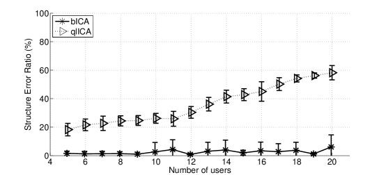
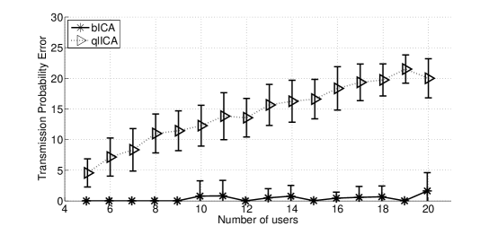
(a) Structure Error Ratio	(b) Transmission Probability Error

Figure 8: Accuracy validation result of two models qlICA and bICA. Result is average of 20 runs with different initial seeds and symmetric error bars indicate standard deviations.

7 Discussion

In this section, we discuss several practical considerations in implementing the proposed algorithms in real systems for wireless monitoring. The primary focus of this work is sniffer-channel assignment given fixed sniffer locations. Sniffer placement has been addressed in [19], which assumes worse case loads in the network, while sniffer-channel assignment can be made based on the actual measured loads. In fact, both problems can be considered in a single optimization framework if we generalize the sniffer placement problem to decide online which set of sniffers should be turned on given budget constraints. Implementation of sniffer-channel assignment should incorporate the learning procedure proposed in [11]. The time granularity of channel assignment should be sufficiently long to amortize the cost due to channel switching. To allow a consistent view of the channel at different locations, clock synchronization across multiple sniffers is needed. While clock synchronization can be performed offline using the frame traces collected [5], the accuracy of clock synchronization directly affects the inference accuracy of the ICA based methods in the sniffer-centric model. The choice of the slot of the binary measurements shall be made that takes into account the persistence of user transmission activities. The channel assignment in its current form is computed in a centralized manner. This is reasonable since the sniffers are likely operated by a single administrative domain. An alternative distributed implementation has been considered in [33] for the user-centric model based on the annealed Gibbs sampler. However, parameters of the distributed algorithm need to be properly tuned for fast convergence (and hence less message exchanges). From our understanding, the sniffer-centric model is not immediately amiable to distributed implementation.

8 Conclusion

In this paper, we formulated the problem of maximizing QoM in multi-channel infrastructure wireless networks with different a priori knowledge. Two different models are considered, which differ by the amount (and type) of information available to the sniffers. We show that when complete information of the underlying cover graph and access probabilities of users are available, the problem is NP-hard, but can be approximated within a constant factor. When only binary information about the channel activities is available to the sniffers, we propose two approaches (qlICA and bICA) so that one can map the problem to the one where complete information is at hand using the statistics of the sniffers’ observations. We further conducted a detail study comparing the performance of qlICA and bICA. Finally, evaluations demonstrate the effectiveness of our proposed inference methods and optimization techniques.

Huy Nguyen received his B.S. degree in Computer Science from University of Science, Ho Chi Minh City, Vietnam, in 2006, and his M.E. degree in Electrical Engineering from Chonnam National University, Guangju, Korea, in 2009. Since 2009, he started pursuing his Ph.D. degree in the Department of Computer Science, University of Houston under the guidance of Prof. Rong Zheng. His research interests include wireless and sensor network management, information diffusion on social networks.

Gabriel Scalosub received his B.Sc. in Mathematics and Philosophy from the Hebrew University of Jerusalem, Israel, in 1996. He received his M.Sc. and Ph.D. in Computer Science from the Technion - Israel Institute of Technology, Haifa, Israel, in 2002 and 2007, respectively. In 2008 he was a postdoctoral fellow at Tel-Aviv University, Israel, and in 2009 he was a postdoctoral fellow at the University of Toronto, Canada. In October 2009 Gabriel Scalosub joined the Department of Communication Systems Engineering at Ben Gurion University of the Negev, Israel. He served on various technical program committees, including Infocom, IWQoS, IFIP-Networking, ICCCN, and WCNC. His research focuses on theoretical algorithmic issues arising in various networking environments, including buffer management, scheduling, and wireless networks. He is also interested in broader aspects of combinatorial optimization, online algorithms, approximation algorithms, and algorithmic game theory.

Rong Zheng (S’03-M’04-SM’10) received her Ph.D. degree from Dept. of Computer Science, University of Illinois at Urbana-Champaign and earned her M.E. and B.E. in Electrical Engineering from Tsinghua University, P.R. China. She is on the faculty of the Department of Computing and Software, McMaster University. She was with University of Houston between 2004 and 2012. Rong Zheng’s research interests include network monitoring and diagnosis, cyber physical systems, and sequential learning and decision theory. She received the National Science Foundation CAREER Award in 2006. She serves on the technical program committees of leading networking conferences including INFOCOM, ICDCS, ICNP, etc. She served as a guest editor for EURASIP Journal on Advances in Signal Processing, Special issue on wireless location estimation and tracking, Elsevler s Computer Communications Special Issue on Cyber Physical Systems; and Program co-chair of WASA’12 and CPSCom’12.

References

- [1] J. Yeo, M. Youssef, and A. Agrawala, “A framework for wireless LAN monitoring and its applications,” in Proceedings of the 3rd ACM Workshop on Wireless Security (WiSE), 2004, pp. 70–79.
- [2] J. Yeo, M. Youssef, T. Henderson, and A. Agrawala, “An accurate technique for measuring the wireless side of wireless networks,” in Proceedings of the 2005 Workshop on Wireless Traffic Measurements and Modeling, 2005, pp. 13–18.
- [3] M. Rodrig, C. Reis, R. Mahajan, D. Wetherall, and J. Zahorjan, “Measurement-based characterization of 802.11 in a hotspot setting,” in Proceedings of the 2005 ACM SIGCOMM Workshop on Experimental Approaches to Wireless Network Design and Analysis, 2005, pp. 5–10.
- [4] Y.-C. Cheng, J. Bellardo, P. Benkö, A. C. Snoeren, G. M. Voelker, and S. Savage, “Jigsaw: solving the puzzle of enterprise 802.11 analysis,” in SIGCOMM, 2006.
- [5] A. Chhetri and R. Zheng, “WiserAnalyzer: A passive monitoring framework for WLANs,” in Proceedings of the 5th International Conference on Mobile Ad-hoc and Sensor Networks (MSN), 2009.
- [6] Y.-C. Cheng, J. Bellardo, P. Benkö, A. C. Snoeren, G. M. Voelker, and S. Savage, “Jigsaw: solving the puzzle of enterprise 802.11 analysis,” SIGCOMM Comput. Commun. Rev., vol. 36, no. 4, pp. 39–50, Aug. 2006.
- [7] K. Premkumar and A. Kumar, “Optimal sleep-wake scheduling for quickest intrusion detection using wireless sensor networks,” in IEEE INFOCOM 2008., april 2008, pp. 1400 –1408.
- [8] M. Kodialam and T. Lakshman, “Detecting network intrusions via sampling: a game theoretic approach,” in INFOCOM 2003, vol. 3, march-3 april 2003, pp. 1880 – 1889 vol.3.
- [9] T. Wang, M. Srivatsa, D. Agrawal, and L. Liu, “Learning, indexing, and diagnosing network faults,” in Proceedings of the 15th ACM SIGKDD, ser. KDD ’09. New York, NY, USA: ACM, 2009, pp. 857–866.
- [10] S. Rayanchu, A. Mishra, D. Agrawal, S. Saha, and S. Banerjee, “Diagnosing wireless packet losses in 802.11: Separating collision from weak signal,” in INFOCOM 2008, april 2008, pp. 735 –743.
- [11] P. Arora, C. Szepesvári, and R. Zheng, “Sequential learning for optimal monitoring of multi-channel wireless networks,” in INFOCOM, 2011, pp. 1152–1160.
- [12] A. Hyvärinen and E. Oja, “Independent component analysis: algorithms and applications,” Neural Networks, vol. 13, no. 4-5, pp. 411–430, 2000.
- [13] H. Nguyen and R. Zheng, “Binary independent component analysis with or mixtures,” IEEE Transactions on Signal Processing, vol. 59, no. 7, pp. 3168–3181, 2011.
- [14] A. Balachandran, G. M. Voelker, P. Bahl, and P. V. Rangan, “Characterizing user behavior and network performance in a public wireless LAN,” SIGMETRICS Perform. Eval. Rev., vol. 30, no. 1, pp. 195–205, 2002.
- [15] T. Henderson, D. Kotz, and I. Abyzov, “The changing usage of a mature campus-wide wireless network,” in Proceedings of the 10th MOBICOM, 2004, pp. 187–201.
- [16] R. Chandra, V. N. Padmanabhan, and M. Zhang, “WiFiProfiler: cooperative diagnosis in wireless LANs,” in Proceedings of the 4th International Conference on Mobile Systems, Applications, and Services (MobiSys), 2006, pp. 205–219.
- [17] Y.-C. Cheng, M. Afanasyev, P. Verkaik, P. Benkö, J. Chiang, A. C. Snoeren, S. Savage, and G. M. Voelker, “Automating cross-layer diagnosis of enterprise wireless networks,” in SIGCOMM, 2007.
- [18] L. Qiu, P. Bahl, A. Rao, and L. Zhou, “Troubleshooting wireless mesh networks,” SIGCOMM Comput. Commun. Rev., vol. 36, no. 5, pp. 17–28, 2006.
- [19] D.-H. Shin and S. Bagchi, “Optimal monitoring in multi-channel multi-radio wireless mesh networks,” in Proceedings of the 10th ACM Interational Symposium on Mobile Ad Hoc Networking and Computing (MobiHoc), 2009, pp. 229–238.
- [20] C. Chekuri and A. Kumar, “Maximum coverage problem with group budget constraints and applications.”
- [21] A. Yeredor, “ICA in boolean XOR mixtures,” in Proceedings of the 7th International Conference on Independent Component Analysis and Signal Separation (ICA), 2007, pp. 827–835.
- [22] F. W. Computer and F. Wood, “A non-parametric bayesian method for inferring hidden causes,” in Proceedings of the 22nd UAI. AUAI Press, 2006, pp. 536–543.
- [23] A. P. Streich, M. Frank, D. Basin, and J. M. Buhmann, “Multi-assignment clustering for boolean data,” in Proceedings of the 26th Annual International Conference on Machine Learning (ICML). New York, NY, USA: ACM, 2009, pp. 969–976.
- [24] A. Kabán and E. Bingham, “Factorisation and denoising of 0-1 data: a variational approach,” Neurocomputing, vol. 71, no. 10-12, pp. 2291–2308, 2009.
- [25] A. A. Garba, R. M. H. Yim, J. Bajcsy, and L. R. Chen, “Analysis of optical CDMA signal transmission: capacity limits and simulation results,” EURASIP Journal on Applied Signal Processing, vol. 2005, pp. 1603–1616, 2005.
- [26] S. Kandeepan, R. Piesiewicz, and I. Chlamtac, “Spectrum sensing for cognitive radios with transmission statistics: Considering linear frequency sweeping,” EURASIP Journal on Wireless Communications and Networking, 2010.
- [27] E. M. Gold, “Complexity of automaton identification from given data,” Information and Control, vol. 37, no. 3, pp. 302–320, 1978.
- [28] M. R. Garey and D. S. Johnson, Computers and Intractability - A Guide to the Theory of NP-Completeness. New York: W.H. Freeman and Company, 1979.
- [29] A. Chhetri, H. Nguyen, G. Scalosub, and R. Zheng, “On quality of monitoring for multi-channel wireless infrastructure networks,” in Procs. of MobiHoc ’10. NY, USA: ACM, 2010, pp. 111–120.
- [30] V. Guruswami and S. Khot, “Hardness of Max 3SAT with no mixed clauses,” in Proceedings of the 20th Annual IEEE Conference on Computational Complexity (CCC), 2005, pp. 154–162.
- [31] A. Srinivasan, “Distributions on level-sets with applications to approximation algorithms.”
- [32] J. Himberg and A. Hyvärinen, “Independent component analysis for binary data: An experimental study,” in Proceedings of the 3rd International Conference on ICA, 2001, pp. 552–556.
- [33] P. Arora, N. Xia, and R. Zheng, “A gibbs sampler approach for optimal distributed monitoring of multi-channel wireless networks,” in Globecom, 2011.