50 pico arcsecond astrometry of pulsar emission

Abstract

We use VLBI imaging of the interstellar scattering speckle pattern associated with the pulsar PSR 0834+06 to measure the astrometric motion of its emission. The $\sim$5AU interstellar baselines, provided by interference between speckles spanning the scattering disk, enable us to detect motions with sub nanoarcsecond accuracy. We measure a small pulse deflection of $\sim 18\pm 2$km (not including geometric uncertainties), which is 100 times smaller than the native resolution of this interstellar interferometer. This implies that the emission region is small, and at an altitude of a few hundred km, with the exact value depending on field geometry. This is substantially closer to the star than to the light cylinder. Future VLBI measurements can improve on this finding. This new regime of ultra-precise astrometry may enable precision parallax distance determination of pulsar binary displacements.

1 Introduction

The quantitative nature of pulsar emission has remained enigmatic for the past half century since its discovery. One limiting step has been the lack of precise data. To achieve sensivity to emission features would require nano or pico arcsecond imaging, which is challenging to achieve. Various attempts have used the interstellar medium as a lens to detect pulse emission motion: Wolszczan & Cordes (1987), Gupta et al. (1999), Johnson et al. (2012), Gwinn et al. (2012). These have resulted in mutually difficult to reconcile conclusions about the effective emission altitude.

More recently, Pen & King (2012) suggested using VLBI resolved images of the ISM scattering to coherently image the pulsar. Brisken et al. (2010) have mapped the individual interstellar lensed images of B0834+06, with precise distances and positions on the sky. These plasma lensed images are separated by many AU. The ultimate objective of such a technique is to use these individual lenses as apertures of a coherent interferometer; in principle, one could reconstruct a full image if the emission region is resolved An easier measurement is the relative phase change during the pulsar rotation, which is presented in this letter.

2 Data

This analysis is based on a recorrelation of data used in Brisken et al. (2010). The voltages of the Arecibo-GBT baselines were recorrelated in gates of 8.9ms width, corresponding to 0.7% of the pulsar period. Only the 3 gates shown in Figure 1 superimposed on the pulse profile showed sufficient signal-to-noise for further processing – the other gates were not used further.

Figure 1: Correlation gates of 9ms width. The 3 gates indicated in the plot are used in this analysis.

The pulsar and lens geometry are known: The pulsar is at a distance of  640 pc (Deller & Brisken, unpublished), and the screen is located a distance of $415\pm 5\,$pc (with this error estimate not including pulsar distance uncertainties). This places the screen two thirds of the way to the pulsar, which improves the angular resolution: The characteristic resolving power of the scattering is $\lambda/D\sim 0.3\,\mu$as for $\lambda\sim 1\,$m and a typical baseline length of 5 AU, corresponding to displacement between major groups of speckles on the scattering disk. With the pulsar located 225 pc from the scattering region, this angular resolution corresponds to a linear scale of 10,000 km. We used a wavelength $\lambda\sim 1$m and $D=$5AU as a reference scale, which is roughly the displacement of a major group of scattering points. Two points at the pulsar separated by 10,000 km differ by 2$\pi$ radians. The native resolution, in this sense, is then $\sim 1700$/SN km, where SN is the signal-to-noise of the measurement. From Earth, this corresponds to a resolution of 100/SN nano arcseconds.

For this analysis, we primarily used data acquired on the Arecibo (AO) – Greenbank (GB) interferometric baseline. The individual dish data was difficult to interpret due to finite bit sampling and local RFI. The only other data used in this analysis was the AO-Jodrell Bank 76m (JB) cross-correlation baseline, needed for the screen image in Section 3. For this baseline, a single gate of width 125 ms spanning the entire on-pulse (taken from the original Brisken et al. (2010) visibility data) was used, since the raw JB voltage data was no longer available for recorrelation.

3 Holography

Our objective is to perform relative astrometry on the pulsar as a function of pulse phase. To increase the sensitivity of our astrometry, we applied a holographic technique to obtain the phase of the pulsar radiation through each scattering image. We used a technique similar to Walker et al. (2008). The basic framework is the same, which we summarize briefly. The dynamic spectrum $I(\nu,t)=\langle v(\nu,t^{\prime})\bar{v}(\nu,t^{\prime})\rangle_{t^{\prime}\sim t}$ is the average modulus of the complex field response.

We call the Fourier transform of the dynamic spectrum, $\tilde{I}(\tau,\omega)$, the conjugate spectrum. This quantity is the auto correlation of the fourier transform of the voltage impulse-response function. Walker et al. (2008) showed that the voltage impulse-response function decomposes into a sparse set in the delay–Doppler rate ($\tau-\omega$) plane. Its modulus is the secondary spectrum, which is a quartic quantity in the impulse-response function.

We show the secondary spectrum summed over all pulse gates in Figure 2. As originally noted by Stinebring et al. (2001), the striking feature is the presence of inverted parabolic arclets.

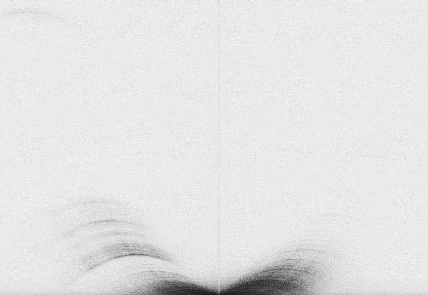
Figure 2: Secondary spectrum. The horizontal axis is $\pm 40$ mHz, the vertical axis extends to 1ms.

In the conjugate spectrum, the modulus is an auto-correlation of the voltage impulse-response function. An isolated inverted arclet corresponds to the correlation of an isolated scattering point with the main scattering disk. By convolving the conjugate spectrum with the complex conjugate of an inverted arclet, we obtain the analogy of a “dirty image” of the holographic impulse-response function.

Unlike the Walker procedure, we do not start with the brightest points in the secondary spectrum. These regions contain contributions from many scattering points, and are maximally degenerate on their own. Instead of decomposing the regions of brightest flux, we start with an isolated inverted arclet in the conjugate spectrum. This arclet is primarily the impulse-response function of the voltage as measured against an isolated scattering point, and allows a solution of the impulse-response function local in the secondary spectrum. We first isolate one, and convolve the conjugate spectrum by it. We then pick an isolated region of bright response points around -20mHz, and stack the arclets weighted by the conjugate of these response points. Figure 3 shows a stack of arclets. These are complex impulse-response functions.

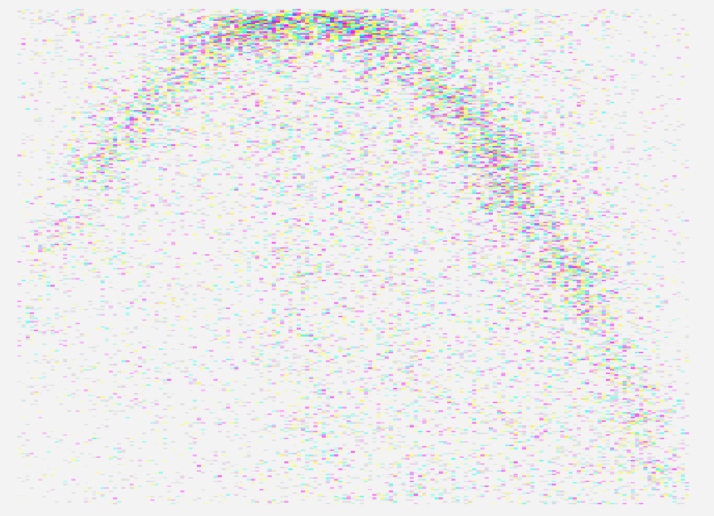
Figure 3: coherently stacked arclets. The colour coding represents the phase. It appears random, but is essential to achieve coherent holography.

The conjugate spectrum is then again convolved, this time with the stacked arclet template. We call this the dirty semi-descattered spectrum, indicating that the complex impulse-response function has been applied once. A cleaned fully descattered spectrum would be a dynamic spectrum which does not scintillate in frequency or time. In principle, this dirty semi-descattered spectrum maximizes the signal-to-noise on each residual in the limit that individual scattering points remain uncorrelated. The result is shown in Figure 4.

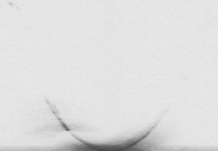
Figure 4: Holographic gate cross spectrum obtained by multiplying the semi descattered conjugate spectrum of gate 1 with the complex conjugate of the corresponding quantity of gate 2. Shown here is the real part.

We see the inverted parabolic arclets descattered onto the main parabola. While the stacked arclets are obtained from the combined gates, we apply this to each gate separately. Then we multiply the conjugate spectrum from one gate by the complex conjugate of the conjugate spectrum from another gate. If these two are statistically identical, the expectation value will be a real number. If there is a systematic phase lag, the imaginary component will not be zero. Initial examination shows the imaginary part of the holographic cross spectrum to be much smaller than the real part, indicating that phase changes are very small. We expect the phase change to be proportionate to the linear separation between images, which is equal to the doppler frequency for this collinear scattering structure.

To estimate the noise in the holographic cross spectrum, we apply a bootstrap technique: for each pair of gates, we generate new gates by randomly selecting scintels from each constituent dynamic spectrum. We then compute the holographic cross spectrum. In this construction, the imaginary part has by construction zero expectation value and a finite variance. We compute the variance at each point from 1000 realizations. Knowing the variance allows us to fit for the phase gradient, and estimate its error. We examined the covariance between bins, which is less than 10% for neighboring bins, and consistent with zero for further separated bins. We thus neglect the covariance, since an inverse of the noise matrix would be very noisy and require many more realizations.

We also used the holographic technique to directly image the pulsar scattering image on the sky. The same procedure results in a semi-descattered VLBI visibility and secondary cross spectrum (Brisken et al., 2010), i.e. a complex value for each doppler frequency and lag. The phase determines the distance along the baseline. We used only the AO-GBT and AO-JB baselines, and interpreted each phase as the distance along the baseline. This is then rebinned onto a 2-D map of the sky, shown in Figure 5

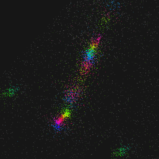
Figure 5: Holographic VLBI image. Imaged formed using the VLBI phase of each holographic cross spectrum residual. The colour is proportionate to time delay, in a periodic hue map. The green locus of points at left center is a sidelobe of the true locus on the lower right. The main base of the parabola as been omitted, which is centered at the origin. This scattering image becomes our celestial interferometer aperture with which we image the pulsar. At a scattering screen distance of $\sim$400 pc, each mas is 0.4 AU.

The map shows a visual representation of the scattering disk obtained this way. This forms the celestial interferometer which we use for astrometry of the pulse emission. This is the aperture of our interstellar interferometer which we will use for precision imaging of the pulsar.

4 Results

In Figure 6 we show the reconstructed pulse motion. The first feature to notice is that the motion is tiny: different gates have almost identical phase responses on the scattering screen to within one percent of a radian. This immediately implies that the motion is less than 30km.

Figure 6: Pulsar motion projected along scattering axis. The horizontal axis is the time difference, the vertical axis is the apparent motion shift along the scattering axis, scaled to a doppler frequency of -15mHz. The changes are always small. The error is about 1/1000th of a radian, wich reflects the extremely high signal-to-noise of the measurement.

This is two orders of magnitude smaller than some previous estimates(Wolszczan & Cordes, 1987; Gupta et al., 1999), albeit for different pulsars, and surprisingly small compared to some size interpretations using the modulation index(Gwinn et al., 2012). Recent modulation analyses have also reported sizes consistent with zero, and smaller than 4km(Johnson et al., 2012). We note that our measurement is differential, relying on only the change of scintillation pattern from gate to gate.

We find the best linear motion fit to be $9\pm 1.1$ km per gate of 9ms, which is an apparent motion of $\sim$ 1000 km/sec. The pulsar motion is $\sim 162\pm 10$ km/sec(Lyne et al., 1982) due north, which projects to $\sim 147$ km/sec along the scattering structure, almost an order of magnitude smaller than the measured motion. We do not correct for this effect.

No motion is observed on the 1ms island, which is at about 45 degrees to the main scattering axis. This island has about 4% of the flux, limiting the motion of the pulse along the dimension transverse to the scattering disk to $\mathrel{\hbox{\hbox to0.0pt{\hbox{\lower 4.0pt\hbox{$\sim$}}\hss}\hbox{$<$}}}35$ km ($2-\sigma$).

5 Interpretation

The direct observable is the apparent motion of the emission region as a function of pulse phase. This can in turn be related to the pulsar emission altitude by specifying the geometry of the emission mechanism. We consider some limits that are exactly calculable. One is the case that the emission region is very small, and the pulse period is determined by the beaming angle of the emission. In this case, the deflection of the pulse is just the height times the duty cycle, corresponding to an emission height of about 200km.

Possibly the extreme antithetical model is one in which the emission is infinitely beamed radiating tangentially to the local magnetic field line. In this case, the altitude is related to the deflection by the field curvature. If we take the curvature to be roughly the altitude, as expected for a dipolar field, we obtain the same rough altitude as above. We note that this can be arbitrarily incorrect: in the unlikely extreme case that the field lines are purely radial with no curvature, there is no apparent motion, and the emission altitude could be arbitrarily high. In the infinite curvature limit, the emission is given by the same altitude as the beamed case.

From these scenarios we also see that the emission region generically has a smaller angular size than the displacement during the pulse: in the infinitely beamed scenario we only see the one field line tangential to our line of sight, resulting in an infinitesimal apparent emission size. In the first scenario, we see all field lines which are within one beaming angle of our line of sight. The size of the emission region plus the beaming angle must be less than the pulse duration, while the deflection is given by the beaming angle. There could be exotic counter examples, for example if the field lines were convergent at the emission region.

6 Conclusions

We have used the interstellar medium is a giant lens to study the motion of the pulsar emission. We have found this motion to be tiny, by more than order of magnitude, compared to previous indirect indications. We expect the apparent size of the emission region to be smaller than the displacement, making the emission essentially unresolvable on these interstellar baselines. More VLBI observations of a range of pulsars at lower frequencies could help improve the situation.

The small nature of the emission region implies that pulsars will be unresolved by all known scattering screens, including the scattering screen at the galactic center(Deneva et al., 2009), and potentially multiple images against a black hole(Rafikov & Lai, 2006).

This new era of precision picoarcsecond astrometry opens the possibilities for precise distance measurements to pulsars. It would increase the sensitivity and angular resolution of pulsar timing arrays to gravitational waves(Boyle & Pen, 2012). The pulsar reflex motion for a binary system provides the appropriate parallax.

7 Acknowledgements

U-LP thanks NSERC and CAASTRO for support.

References

- Boyle & Pen (2012) Boyle L., Pen U.-L., 2012, Phys. Rev. D , 86, 124028
- Brisken et al. (2010) Brisken W. F., Macquart J.-P., Gao J. J., Rickett B. J., Coles W. A., Deller A. T., Tingay S. J., West C. J., 2010, ApJ, 708, 232
- Deneva et al. (2009) Deneva J. S., Cordes J. M., Lazio T. J. W., 2009, ApJ, 702, L177
- Gupta et al. (1999) Gupta Y., Bhat N. D. R., Rao A. P., 1999, ApJ, 520, 173
- Gwinn et al. (2012) Gwinn C. R., Johnson M. D., Reynolds J. E., Jauncey D. L., Tzioumis A. K., Hirabayashi H., Kobayashi H., Murata Y., Edwards P. G., Dougherty S., Carlson B., del Rizzo D., Quick J. F. H., Flanagan C. S., McCulloch P. M., 2012, ApJ, 758, 7
- Johnson et al. (2012) Johnson M. D., Gwinn C. R., Demorest P., 2012, ApJ, 758, 8
- Lyne et al. (1982) Lyne A. G., Anderson B., Salter M. J., 1982, MNRAS, 201, 503
- Pen & King (2012) Pen U.-L., King L., 2012, MNRAS, 421, L132
- Rafikov & Lai (2006) Rafikov R. R., Lai D., 2006, Phys. Rev. D , 73, 063003
- Stinebring et al. (2001) Stinebring D. R., McLaughlin M. A., Cordes J. M., Becker K. M., Goodman J. E. E., Kramer M. A., Sheckard J. L., Smith C. T., 2001, ApJ, 549, L97
- Walker et al. (2008) Walker M. A., Koopmans L. V. E., Stinebring D. R., van Straten W., 2008, MNRAS, 388, 1214
- Wolszczan & Cordes (1987) Wolszczan A., Cordes J. M., 1987, ApJ, 320, L35