Characterizing Magnetized Turbulence in M51

Abstract

We use previously published high-resolution synchrotron polarization data to perform an angular dispersion analysis with the aim of charactering magnetized turbulence in M51. We first analyze three distinct regions (the center of the galaxy, and the northwest and southwest spiral arms) and can clearly discern the turbulent correlation length scale from the width of the magnetized turbulent correlation function for two regions and detect the imprint of anisotropy in the turbulence for all three. Furthermore, analyzing the galaxy as a whole allows us to determine a two-dimensional Gaussian model for the magnetized turbulence in M51. We measure the turbulent correlation scales parallel and perpendicular to the local mean magnetic field to be, respectively, $\delta_{\|}=98\pm 5$ pc and $\delta_{\bot}=54\pm 3$ pc, while the turbulent to ordered magnetic field strength ratio is found to be $B_{\mathrm{t}}/B_{0}=1.01\pm 0.04$. These results are consistent with those of Fletcher et al. (2011), who performed a Faraday rotation dispersion analysis of the same data, and our detection of anisotropy is consistent with current magnetized turbulence theories.

1 Introduction

The magnetized diffuse interstellar medium, of the Milky Way and other galaxies, is turbulent and so an understanding of its properties and role should include the quantities commonly used to describe turbulence: characteristic length scales, power spectra, the relative energies in the mean and fluctuating components, and so on. One important property of magnetohydrodynamic (MHD) turbulence is that the random fluctuations in the inertial range are not necessarily isotropic, as is the case in the classical picture of purely hydrodynamic, incompressible Kolmogorov turbulence: the correlation length of magnetic fluctuations can be larger along the mean field direction compared to the perpendicular direction. This mean field can be either an external large-scale magnetic field or simply the magnetic field at the largest scale of a turbulent eddy acting on fluctuations within the eddy on smaller scales. As well as the inherent anisotropy of MHD turbulence dynamical effects in the ISM flow such as shocks and shear, due to localized sources such as supernovae or global features like differential rotation, can also imprint anisotropy on the turbulence.

There have been a few indications from observations that magnetic field fluctuations in the ISM exhibit anisotropies. Brown & Taylor (2001) binned Faraday rotation measures (RM) for extra-galactic (EG) sources in the Galactic plane in the range $82\deg<l<146\deg$ and found that the variance in a bin is correlated with the magnitude of the mean RM; higher RMs are associated with stronger fluctuations, and it was proposed that this occurs because the fluctuations in the magnetic field are mainly aligned with the mean field. Jaffe et al. (2010) fitted a model magnetic field to the synchrotron emission and EG RMs along the Galactic plane and found that an anisotropic (or in their terminology an ordered random) magnetic field component was required to fit the observations along with both a mean field and an isotopic random magnetic field. Similarly, Jansson & Farrar (2012) required either an anisotropic (or striated field in their terminology) magnetic field component, or a correlation between the mean magnetic field and cosmic ray density, to obtain good fits to all-sky observations of synchrotron emission and RMs (in their model anisotropic random fields and close cosmic ray-to-mean magnetic field coupling are degenerate parameters). Away from the Milky Way, Beck et al. (2005) compared the observed increase in both total and polarized synchrotron emission at the strong shock fronts along the bars of the galaxies NGC 1097 and NGC 1365 with theoretical expectations based on the compression and shear of random and mean magnetic fields; their results indicate that strong anisotropic random magnetic fields are produced at these positions. Fletcher et al. (2011) attributed the order of magnitude difference between ordered magnetic field strengths obtained via equipartition estimates and Faraday rotation modeling, to a strong anisotropic random magnetic field in the nearby galaxy M51: this component is responsible for the strong polarized signal but contributes little to the Faraday rotation.

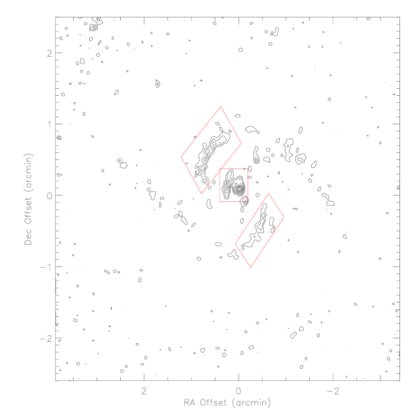
Figure 1: Polarized flux at $\lambda 6.2$ cm for M51. There are three regions that can be independently used (or combined) for a dispersion analysis: the spiral arms in the northeast and southwest, and the center of the galaxy. These regions are contained within the corresponding three red rectangles in the figure. The map is centered at $\mathrm{RA\,}(\mathrm{J2000})=11^{\mathrm{h}}29^{\mathrm{m}}52\fs 4$, $\mathrm{Dec\,}(\mathrm{J2000})=47^{\circ}11\arcmin 43\farcs 5$, and the contours are drawn at 20 to 80 percent (10 percent increments) of the peak polarized flux density ($173\,\mu$Jy/beam).

In this paper we perform an angular dispersion analysis, based on the work of Falceta-Gonçalves et al. (2008), Hildebrand et al. (2009), and Houde et al. (2009, 2011), on the Effelsberg 100-m/VLA $\lambda 6.2$ cm synchrotron polarization map of Fletcher et al. (2011) ($4\arcsec$ FWHM resolution and $1\arcsec$ sampling). We show in Figure 1 the global view of M51 in polarized flux provided by these data. There are clearly only three regions that can be used, or combined, for a dispersion analysis: the spiral arms in the northeast and southwest, and the center of the galaxy. These regions are contained within the corresponding three red rectangles in the figure.

Although these data were obtained with high spatial resolution, they will not allow us to get a handle on the magnetized turbulence power spectrum as done in Houde et al. (2011) for Galactic molecular clouds (note that $1\arcsec\simeq 37$ pc). Nonetheless, Fletcher et al. (2011) calculate from a Faraday rotation dispersion analysis that the size of a turbulence cell should be approximately 50 pc. This suggests that we may be able to measure and determine this value independently with the data at hand, given the expected size of a cell and the aforementioned spatial resolution. We would be in a position to not only determine the number of turbulence cells contained in the average column of gas subtended by the telescope beam, but also get accurate values for the ratio of the turbulent-to-ordered magnetic energy in different parts of M51. Furthermore, in view of the large numbers of polarization measurements available with this map the statistics may be good enough to allow a study of possible anisotropy in the autocorrelation function of magnetized turbulence.

We start in the next section by first giving a summary of the dispersion analysis in Section 2, a description of the data used for our analysis is given in Section 3, which is then followed in Section 4.1 by an isotropic dispersion analysis on the three available regions in the manner presented in Houde et al. (2009, 2011) and Hildebrand et al. (2009). A first attempt at measuring any potential anisotropy is presented in Section 4.2.1 through the independent analyses on displacement vectors that are grouped into two sets, which are either oriented approximately parallel or perpendicular to the local mean magnetic field. The derived turbulence autocorrelation functions can then be compared and any differences in their widths will reveal an anisotropy. Finally, in Section 4.2.2 we apply the dispersion analysis to M51 as a whole (i.e., by simultaneously using all available polarization vectors) to map the two-dimensional turbulence autocorrelation function to once again reveal any anisotropy in the magnetized turbulence, but in more detail. We finish with a discussion of our results in Section 5, a brief summary in Section 6, while more details concerning the dispersion analysis will be found in the Appendix.

2 Angular Dispersion Analysis

Structure functions have long been used in physics and astrophysics to characterize turbulence, as they allow for the treatment of power-law energy spectra, such as those found in Kolmogorov turbulence, without the mathematical divergences associated with stationary signal (Frisch, 1995; Beck et al., 1999; Falceta-Gonçalves et al., 2008). Such structure functions, of varying orders, can be calculated for a range of physical parameters (e.g., velocity and density fields). In this paper, we intend to apply the angular dispersion analysis previously introduced in the literature (Falceta-Gonçalves et al., 2008; Hildebrand et al., 2009; Houde et al., 2009, 2011), where the chosen parameter is the orientation of the projection of the magnetic field on the plane of the sky. More precisely, we will use the polarization angle orientation in lieu of that of the magnetic field. For the polarization of synchrotron (or dust) emission this angle is orientated at $90^{\circ}$ from that of the projected magnetic field. Although we will provide a summary of the important relations required for the angular dispersion analysis later in Section 2.2, a simplified exposition based on material that can be found in Hildebrand et al. (2009) is first given here.

2.1 Angular Structure Function

We start by defining the difference $\Delta\Phi\left(\boldsymbol{\ell}\right)$ in the orientation of the magnetic field (unless otherwise specified, in this paper we will only concern ourselves with the plane of the sky component of the magnetic field) at two points separated by a distance $\boldsymbol{\ell}$

$$\Delta\Phi\left(\boldsymbol{\ell}\right)\equiv\Phi\left(\mathbf{r}\right)-\Phi\left(\mathbf{r}+\boldsymbol{\ell}\right),$$ (1)

with $\Phi\left(\mathbf{r}\right)$ the magnetic field orientation at position $\mathbf{r}$ (both $\mathbf{r}$ and $\boldsymbol{\ell}$ are also understood to be located in the plane of the sky). Given a set of measurements $\Phi\left(\mathbf{r}\right)$ on a polarization map, we can also define the following (second order) angular structure function

$$\left\langle\Delta\Phi^{2}\left(\ell\right)\right\rangle\equiv\frac{1}{N\left(\ell\right)}\sum_{i=1}^{N\left(\ell\right)}\left[\Phi\left(\mathbf{r}\right)-\Phi\left(\mathbf{r}+\boldsymbol{\ell}\right)\right]^{2}$$ (2)

where $\left\langle\cdots\right\rangle$ denotes an average, $N\left(\ell\right)$ is the number of pairs of field orientation measurements separated by $\ell=\left|\boldsymbol{\ell}\right|$, and stationarity and isotropy were assumed (i.e., the structure function is only dependent on the magnitude of $\boldsymbol{\ell}$, and not on its orientation or $\mathbf{r}$; see Falceta-Gonçalves et al. 2008; Hildebrand et al. 2009).

Figure 2: An example of an angular structure function. Panel a) shows hypothetical turbulent $\left\langle\Delta\Phi_{\mathrm{t}}^{2}\left(\ell\right)\right\rangle$ (triple-dot-broken curve) and ordered $\left\langle\Delta\Phi_{0}^{2}\left(\ell\right)\right\rangle$ (dot-broken curve) contributions to the total angular structure function $\left\langle\Delta\Phi^{2}\left(\ell\right)\right\rangle$ plotted in Panel b) (solid curve). Panel c) presents the same information as Panel b) but displayed as a function of $\ell^{2}$ instead of $\ell$. The total angular structure function is subtracted from a Taylor series fit obtained from its values at $\ell\geq 6\arcsec$ (dot-broken curve in Panels b) and c)) to get the turbulent autocorrelation function shown in Panel d). The correlation length characterizing turbulence is represented by $\delta$.

The main assumption in our analysis consists in modeling the magnetic field, and therefore its orientation through $\Phi\left(\mathbf{r}\right)$, as being composed of a large-scale, ordered component $\Phi_{0}\left(\mathbf{r}\right)$ and a smaller scale, zero-mean, turbulent component $\Phi_{\mathrm{t}}\left(\mathbf{r}\right)$. That is, we write

$$\Phi\left(\mathbf{r}\right)=\Phi_{\mathrm{t}}\left(\mathbf{r}\right)+\Phi_{0}\left(\mathbf{r}\right),$$ (3)

which, if we further assume these two components to be statistically independent, leads to

$$\left\langle\Delta\Phi^{2}\left(\ell\right)\right\rangle=\left\langle\Delta\Phi_{\mathrm{t}}^{2}\left(\ell\right)\right\rangle+\left\langle\Delta\Phi_{0}^{2}\left(\ell\right)\right\rangle.$$ (4)

We thus find that the structure function is composed of two angular components stemming from the contributions of the turbulent and ordered magnetic fields. Our assumption on the difference between the two scales therefore allows for their separation and analyses. This is exemplified in Figure 2 where we show (Panel a)) hypothetical turbulent and ordered contributions to the total angular structure function (Panel b), solid curve), as expressed in Equation (4). Panel c) presents the same information as Panel b) for $\left\langle\Delta\Phi^{2}\left(\ell\right)\right\rangle$ but displayed as a function of $\ell^{2}$ instead of $\ell$. This is to show that the separation of the two length scales is sometimes easier to visualize, through the abrupt change in the slope of $\left\langle\Delta\Phi^{2}\left(\ell\right)\right\rangle$, by using the square of the distance for the abscissa; we will use both representations for the data analyzed later in this paper. The total angular structure function (of Panels b) or c)) is the input to our problem as obtained from a polarization map, which we seek to analyze in order to characterize magnetized turbulence.

The behavior of turbulent and ordered contributions to the total angular structure function of Panel a) can be qualitatively understood from the fact that, evidently, they must equal zero when $\ell=0$ and then initially increase with $\ell$. The turbulent structure function will keep increasing until it reaches values for $\ell$ that sufficiently exceed the turbulence correlation length $\delta$, at which point it will reach its maximum value. This can also be understood more quantitatively with the following relation

$$\left\langle\Delta\Phi_{\mathrm{t}}^{2}\left(\ell\right)\right\rangle = \left\langle\left[\Phi_{\mathrm{t}}\left(\mathbf{r}\right)-\Phi_{\mathrm{t}}\left(\mathbf{r}+\boldsymbol{\ell}\right)\right]^{2}\right\rangle$$ (5)

$$= 2\left[\left\langle\Phi_{\mathrm{t}}^{2}\left(0\right)\right\rangle-\left\langle\Phi_{\mathrm{t}}^{2}\left(\ell\right)\right\rangle\right],$$

where the (stationary and isotropic) turbulent autocorrelation function is defined with

$$\left\langle\Phi_{\mathrm{t}}^{2}\left(\ell\right)\right\rangle\equiv\left\langle\Phi_{\mathrm{t}}\left(\mathbf{r}\right)\Phi_{\mathrm{t}}\left(\mathbf{r}+\boldsymbol{\ell}\right)\right\rangle.$$ (6)

It therefore follows that $\left\langle\Delta\Phi_{\mathrm{t}}^{2}\left(\ell\right)\right\rangle=2\left\langle\Phi_{\mathrm{t}}^{2}\left(0\right)\right\rangle$ when $\ell\gg\delta$, as the turbulence is not correlated on such scales and its autocorrelation vanishes. The ordered structure function is expected to rise, at first monotonically, with increasing values of $\ell$ in view of its larger-scale nature. For the example of Figure 2 we have characterized the turbulent component with a Gaussian autocorrelation function of width, or correlation length (i.e., its standard deviation) $\delta=2\arcsec$, while the ordered structure function was modeled with a Taylor expansion in powers of $\ell^{2}$. This restriction to even powers in $\ell$ is dictated from the assumption of isotropy for the structure function.

With the previous assumption in the difference of the two length scales it becomes possible to model the ordered component $\left\langle\Delta\Phi_{0}^{2}\left(\ell\right)\right\rangle$ independently of $\left\langle\Delta\Phi_{\mathrm{t}}^{2}\left(\ell\right)\right\rangle$ by using values of $\ell$ sufficiently large (i.e., sufficiently greater than $\delta$) where any variation in $\left\langle\Delta\Phi_{\mathrm{t}}^{2}\left(\ell\right)\right\rangle$ is negligible. For our example, we chose $\ell\geq 6\arcsec$ to obtain the Taylor series fit given by the dot-broken curve in Panels b) and c) of Figure 2. This curve is then representative of $\left\langle\Delta\Phi_{0}^{2}\left(\ell\right)\right\rangle$ but shifted up by the constant level of the turbulent component present in that range. More precisely if we define a function $\chi\left(\ell\right)$ for this curve, then we write

$$\chi\left(\ell\right)=2\left\langle\Phi_{\mathrm{t}}^{2}\left(0\right)\right\rangle+\left\langle\Delta\Phi_{0}^{2}\left(\ell\right)\right\rangle.$$ (7)

In this paper we will focus on characterizing magnetized turbulence and we are thus interested in isolating the turbulent component of the structure function, or, alternatively, its autocorrelation. The latter (multiplied by a factor of two) is readily evaluated from Equations (4), (5), and (7) with

$$2\left\langle\Phi_{\mathrm{t}}^{2}\left(\ell\right)\right\rangle=\chi\left(\ell\right)-\left\langle\Delta\Phi^{2}\left(\ell\right)\right\rangle$$ (8)

and shown in Panel d) of Figure 2 (i.e., as the subtraction of the solid curve from the dot-broken curve in Panel b)).

Although we could very well use the angular structure function in the manner presented in this section for our analyses of the M51 data, we will nonetheless for the rest of our discussion focus instead on the angular dispersion function $1-\left\langle\cos\left[\Delta\Phi\left(\ell\right)\right]\right\rangle$. We note, however, that the properties, method, and technique discussed thus far for the structure function apply just as well to the dispersion function. In fact, we note that the two angular functions are simply related through

$$1-\left\langle\cos\left[\Delta\Phi\left(\ell\right)\right]\right\rangle\simeq\frac{1}{2}\left\langle\Delta\Phi^{2}\left(\ell\right)\right\rangle$$ (9)

when $\Delta\Phi\left(\ell\right)\ll 1$. The advantage of the dispersion function is its close connection to the autocorrelation of the magnetic field (see Equation (10) below), which then naturally leads to the study of the magnetized turbulent power spectrum through a simple Fourier transform (Houde et al., 2011).

Finally, it is important to note that in general the width of the turbulent autocorrelation function (and of the associated structure/dispersion function) is not solely due to the intrinsic correlation length of turbulence. A correlation scale brought about by the finite spatial resolution with which observations are realized will also combine to the intrinsic turbulent correlation length to set the overall width of the turbulent autocorrelation function. A further complication results from the related problem of signal integration through the line of sight. As we will soon see, a careful analysis of such effects will not only allow us to disentangle the intrinsic correlation length characterizing magnetized turbulence from the overall width of the turbulent autocorrelation function, but also to determine the level of turbulent energy contained in the medium probed by the observations. For this to be feasible, however, some approximation must be made on the nature of the turbulent autocorrelation function. The case of isotropic Gaussian turbulence and beam profile functions was treated in the details in Houde et al. (2009) (see their Section 2) and their main relations detailing the combination of the two length scales for the analysis of turbulence are given in the next section (see Equations (22)-(24) below). In this paper, we further provide an analysis of the more general case of anisotropic Gaussian turbulence in the Appendix, while the corresponding results are also summarized in Section 2.2 (see Equations (19)-(21)). This will in turn make possible the measurement of anisotropy in the turbulent autocorrelation function, which is another important parameter for the characterization of magnetized turbulence.

2.2 Angular Dispersion Function

As previously mentioned, the analysis of the angular dispersion function found in the Appendix and summarized in this section follows that presented in Section 2 of Houde et al. (2009) with the difference that we now allow for the presence of anisotropy in the turbulence. As stated in Section 2.1, we are interested in the function $\cos\left[\Delta\Phi\left(\boldsymbol{\ell}\right)\right]$ that is related to the magnetic field autocorrelation function through

$$\left\langle\cos\left[\Delta\Phi\left(\boldsymbol{\ell}\right)\right]\right\rangle=\frac{\left\langle\overline{\mathbf{B}}\mathbf{\cdot}\overline{\mathbf{B}}\mathbf{\left(\boldsymbol{\ell}\right)}\right\rangle}{\left\langle\overline{\mathbf{B}}\mathbf{\cdot}\overline{\mathbf{B}}\left(0\right)\right\rangle},$$ (10)

where $\left\langle\cdots\right\rangle$ denotes an average and $\left\langle\overline{\mathbf{B}}\mathbf{\cdot}\overline{\mathbf{B}}\mathbf{\left(\boldsymbol{\ell}\right)}\right\rangle\equiv\left\langle\overline{\mathbf{B}}\left(\mathbf{r}\right)\mathbf{\cdot}\overline{\mathbf{B}}\mathbf{\left(\mathbf{r}+\boldsymbol{\ell}\right)}\right\rangle$. It is important to note that the magnetic field $\overline{\mathbf{B}}$ is a weighted average (with the polarized flux) through the thickness of the column of gas probed (i.e., the disk of M51) and across the telescope beam (see Equation (A1)). The local, non-averaged, magnetic field $\mathbf{B\left(\mathbf{x}\right)}$ at a point $\mathbf{x}$ is composed of an ordered field $\mathbf{B}_{0}\mathbf{\left(\mathbf{x}\right)}$ and a turbulent component $\mathbf{B_{\mathrm{t}}\left(\mathbf{x}\right)}$ such that

$$\mathbf{\mathbf{B\left(\mathbf{x}\right)}}=\mathbf{B}_{0}\mathbf{\mathbf{\mathbf{\left(\mathbf{x}\right)+\mathbf{B}_{\mathrm{t}}\left(\mathbf{x}\right)}}}.$$ (11)

As was the case earlier, the displacement vector $\boldsymbol{\ell}$ in Equation (10), and others that will follow, is understood to be located in the plane of the sky. We will further break $\boldsymbol{\ell}$ down into two perpendicular components

$$\boldsymbol{\ell}=\boldsymbol{\ell}_{1}+\boldsymbol{\ell}_{2},$$ (12)

where, unless otherwise noted, $\boldsymbol{\ell}_{1}$ and $\boldsymbol{\ell}_{2}$ are taken to be respectively perpendicular and parallel to the projection of the ordered component of the magnetic field $\mathbf{B}_{0}$ on the plane of the sky. For everything that follows statistical independence between $\mathbf{B}_{0}\mathbf{\left(\mathbf{x}\right)}$ and $\mathbf{B_{\mathrm{t}}\left(\mathbf{x}\right)}$, homogeneity in the strength of the magnetic fields $\left\langle B_{0}^{2}\right\rangle\equiv\left\langle\mathbf{B}_{0}\mathbf{\cdot}\mathbf{B}_{0}\left(0\right)\right\rangle$ and $\left\langle B_{\mathrm{t}}^{2}\right\rangle\equiv\left\langle\mathbf{B}_{\mathrm{t}}\mathbf{\cdot}\mathbf{B}_{\mathrm{t}}\left(0\right)\right\rangle$, as well as, more generally, stationarity in the autocorrelation functions $\left\langle\mathbf{B}_{0}\mathbf{\cdot}\mathbf{B}_{0}\mathbf{\left(\boldsymbol{\ell}\right)}\right\rangle$ and $\left\langle\mathbf{B}_{\mathrm{t}}\mathbf{\cdot}\mathbf{B}_{\mathrm{t}}\mathbf{\left(\boldsymbol{\ell}\right)}\right\rangle$ are assumed. The assumption of homogeneity in the field strength in particular, while clearly an idealization, is needed for securing a quantitative measure of turbulence from our data (see the Appendix for more details).

Using these assumptions it can be shown that, just as was the case for the structure function in Equation (4), the dispersion function $1-\left\langle\cos\left[\Delta\Phi\left(\boldsymbol{\ell}\right)\right]\right\rangle$ can be decomposed into turbulent and ordered terms

$$1-\left\langle\cos\left[\Delta\Phi\left(\boldsymbol{\ell}\right)\right]\right\rangle = \left[b^{2}\left(0\right)-b^{2}\left(\boldsymbol{\ell}\right)\right]+\left[\alpha^{2}\left(0\right)-\alpha^{2}\left(\boldsymbol{\ell}\right)\right]$$ (13)

$$= \left\{b^{2}\left(0\right)+\left[\alpha^{2}\left(0\right)-\alpha^{2}\left(\boldsymbol{\ell}\right)\right]\right\}-b^{2}\left(\boldsymbol{\ell}\right),$$

with the normalized ordered and turbulent autocorrelation functions given by

$$\alpha^{2}\left(\boldsymbol{\ell}\right) = \frac{\left\langle\overline{\mathbf{B}}_{0}\mathbf{\cdot}\overline{\mathbf{B}}_{0}\left(\boldsymbol{\ell}\right)\right\rangle}{\left\langle\overline{\mathbf{B}}\mathbf{\cdot}\overline{\mathbf{B}}\left(0\right)\right\rangle}$$ (14)

$$b^{2}\left(\boldsymbol{\ell}\right) = \frac{\left\langle\overline{\mathbf{B}}_{\mathrm{t}}\mathbf{\cdot}\overline{\mathbf{B}}_{\mathrm{t}}\left(\boldsymbol{\ell}\right)\right\rangle}{\left\langle\overline{\mathbf{B}}\mathbf{\cdot}\overline{\mathbf{B}}\left(0\right)\right\rangle},$$ (15)

respectively. The quantity $b^{2}\left(0\right)$ in Equation (13) is simply, from Equation (15), the integrated turbulent to total magnetic energy ratio. It is also the equivalent of $\left\langle\Delta\Phi_{\mathrm{t}}^{2}\left(\ell\right)\right\rangle$ (see Equation (6)) when dealing with the angular structure function. The ordered function $\alpha^{2}\left(0\right)-\alpha^{2}\left(\boldsymbol{\ell}\right)$, which we assume to be of a larger spatial scale than $b^{2}\left(\boldsymbol{\ell}\right)$, can be advantageously modeled with a Taylor series. Since, as we will soon discuss, we adopt a model of turbulence where the autocorrelation function is even in directions parallel and perpendicular to the projection of $\mathbf{B}_{0}$ on the plane of the sky, it follows that we can write

$$\alpha^{2}\left(0\right)-\alpha^{2}\left(\boldsymbol{\ell}\right)=\sum_{\stackrel{{\scriptstyle{\scriptstyle i+j=1}}}{{i,j\geq 0}}}^{\infty}a_{2i,2j}\ell_{1}^{2i}\ell_{2}^{2j}.$$ (16)

Accordingly, we will proceed by fitting the part within curly braces in Equation (13) using

$$b^{2}\left(0\right)+\left[\alpha^{2}\left(0\right)-\alpha^{2}\left(\boldsymbol{\ell}\right)\right]=b^{2}\left(0\right)+\sum_{\stackrel{{\scriptstyle{\scriptstyle i+j=1}}}{{i,j\geq 0}}}^{\infty}a_{2i,2j}\ell_{1}^{2i}\ell_{2}^{2j}$$ (17)

to the data for high enough values of $\ell\equiv\left|\boldsymbol{\ell}\right|$ where we expect $b^{2}\left(\boldsymbol{\ell}\right)$ to be negligible (i.e., $b^{2}\left(\boldsymbol{\ell}\right)$ dominates at lower values of $\ell$). We will then obtain $b^{2}\left(\boldsymbol{\ell}\right)$ by subtracting the dispersion function data (i.e., the left hand side of Equation (13)) from the aforementioned fit. This function is the equivalent to Equation (7) for $\chi\left(\ell\right)$ defined in Section 2.1 for the angular structure function analysis.

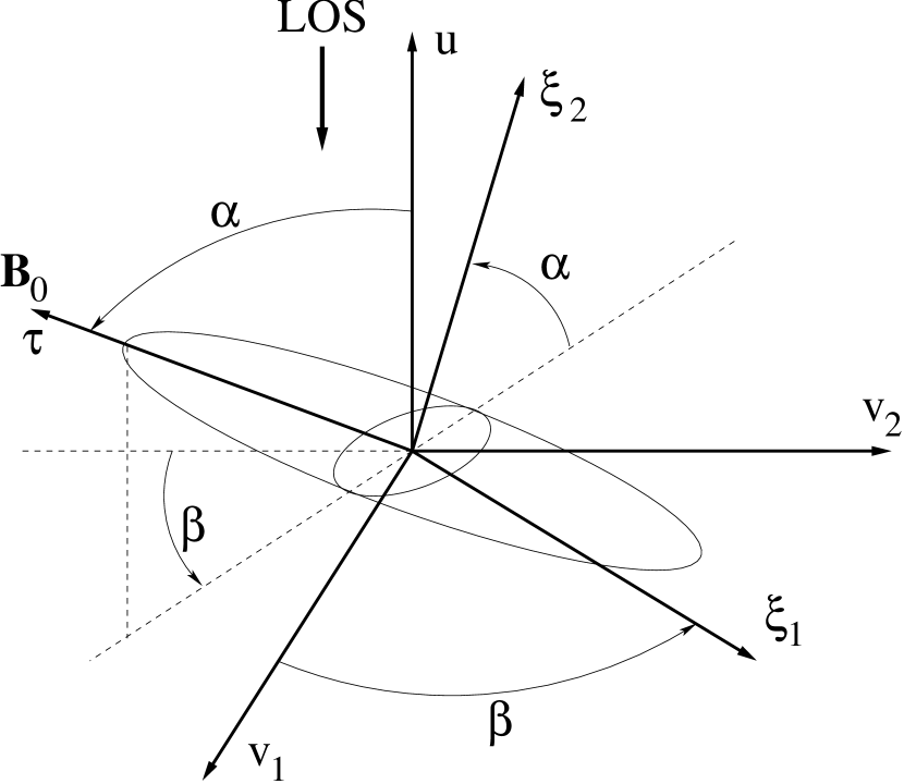
Figure 3: Orientation of the Gaussian ellipsoid characterizing our idealization of magnetized turbulence in the $\left(v_{1},v_{2},u\right)$ coordinate system. The $v_{1}$ and $v_{2}$ axes define the plane of the sky while the line of sight point along the negative $u$-axis. The inclination angle relative to the line of sight of the ellipsoid symmetry axis (and of $\mathbf{B}_{0}$) is given by $\alpha$ while the angle $\beta$ defines the orientation of its projection on the plane of the sky.

We now adopt a picture for magnetized turbulence consistent with current models, either incompressible (Goldreich & Sridhar, 1995) or compressible (Cho & Lazarian, 2003; Kowal & Lazarian, 2010). That is, we will assume that some anisotropy is present in the magnetized turbulent autocorrelation function where it is expected that the correlation lengths in directions parallel and perpendicular to the ordered magnetic field are different. Although this is undoubtedly an idealization, we model the intrinsic autocorrelation function of the magnetized turbulence as an ellipsoid Gaussian function, with the symmetry axis of the ellipsoid aligned with the ordered magnetic field $\mathbf{B}_{0}$ (see Fig. 3). It is possible to analytically solve for $b^{2}\left(\boldsymbol{\ell}\right)$ for such cases with the further assumption that the telescope beam profile is circular Gaussian in form

$$H\left(\mathbf{r}\right)=\frac{1}{2\pi W^{2}}e^{-r^{2}/2W^{2}},$$ (18)

with $W=0.425\>\mathrm{FWHM}$ the beam radius (i.e., it is not the beam’s FWHM but its “standard deviation” equivalent). A general solution for $b^{2}\left(\boldsymbol{\ell}\right)$ when the magnetized autocorrelation function ellipsoid is at arbitrary inclination relative to the line of sight and arbitrary projected orientation on the plane of the sky can be derived and is given in the Appendix.

For M51 we will limit ourselves to three cases. One has the ellipsoid symmetry axis (and the ordered magnetic field $\mathbf{B}_{0}$) at an inclination angle $\alpha$ relative to the line of sight and its projection on the plane of the sky advantageously aligned with one of the observers coordinate axes (still on the plane of the sky; see the Appendix). The integrated (or beam-broadened) autocorrelation function is then analytically expressed by

$$b^{2}\left(\boldsymbol{\ell}\right)=\left[\frac{\left\langle B_{\mathrm{t}}^{2}\right\rangle}{N\left\langle B_{0}^{2}\right\rangle+\left\langle B_{\mathrm{t}}^{2}\right\rangle}\right]e^{-\frac{1}{2}\left[\ell_{1}^{2}/\left(\delta_{\bot}^{2}+2W^{2}\right)+\ell_{2}^{2}/\left(\mu_{2}^{2}+2W^{2}\right)\right]},$$ (19)

where the number of turbulence cells contained in the gas probed by the telescope beam is given by

$$N=\frac{\sqrt{\left(\delta_{\bot}^{2}+2W^{2}\right)\left(\mu_{2}^{2}+2W^{2}\right)}\,\Delta^{\prime}}{\sqrt{2\pi}\delta_{\|}\delta_{\bot}^{2}},$$ (20)

with

$$\mu_{2}^{2}=\delta_{\|}^{2}\sin^{2}\left(\alpha\right)+\delta_{\bot}^{2}\cos^{2}\left(\alpha\right)$$ (21)

and $\delta_{\|}$ and $\delta_{\bot}$ the turbulent correlations lengths parallel and perpendicular to the (local) ordered magnetic field $\mathbf{B}_{0}$, respectively. The inverse of these correlation lengths are, in effect, the corresponding widths of the associated turbulent power spectrum (see the Equation (A7) and the associated discussion in the Appendix). We once again emphasize that, in Equation (19), $\ell_{1}$ and $\ell_{2}$ are the displacements respectively perpendicular and parallel to the projection of $\mathbf{B}_{0}$ on the plane of the sky. In Equation (20) $\Delta^{\prime}$ is the effective depth of the column of polarized gas probed by the telescope beam (Houde et al. 2009; see their Section 3.2 and Equation (45)). This elliptical Gaussian turbulence case will actually be the last one considered in Section 4.2.2.

The first case considered (in Section 4.1) will be for isotropic turbulence when $\delta_{\|}=\delta_{\bot}\equiv\delta$; Equations (19) and (20) then reduce to

$$b^{2}\left(\ell\right)=\left[\frac{\left\langle B_{\mathrm{t}}^{2}\right\rangle}{N\left\langle B_{0}^{2}\right\rangle+\left\langle B_{\mathrm{t}}^{2}\right\rangle}\right]e^{-\ell^{2}/2\left(\delta^{2}+2W^{2}\right)}$$ (22)

and

$$N=\frac{\left(\delta^{2}+2W^{2}\right)\Delta^{\prime}}{\sqrt{2\pi}\delta^{3}}.$$ (23)

Equation (16) is furthermore simplified to

$$\alpha^{2}\left(0\right)-\alpha^{2}\left(\ell\right)=\sum_{j=1}^{\infty}a_{2j}\ell^{2j}.$$ (24)

This isotropic Gaussian turbulence is the model previously solved and used in Houde et al. (2009).

Also, in Section 4.2.1 we consider what could be termed as an “hybrid” model of anisotropic turbulence where Equations (22) - (24) for isotropic turbulence are applied to independent analyses on displacement vectors that are grouped in sets oriented approximately parallel or perpendicular to the local mean magnetic field. Differences in the width of the two turbulent autocorrelation functions can then reveal anisotropy in the magnetized turbulence.

For all three cases, the parameters measurable by fitting the integrated turbulent autocorrelation data with Equation (19) (or Equation (22)) are the correlation lengths $\delta_{\|}$ and $\delta_{\bot}$ (or simply $\delta$), and the intrinsic turbulent-to-ordered magnetic energy ratio $\left\langle B_{\mathrm{t}}^{2}\right\rangle/\left\langle B_{0}^{2}\right\rangle$ (we assume that $\Delta^{\prime}$ and the inclination angle $\alpha$ are known a priori).

3 Observations

In this paper we use the high resolution radio polarization observations of Fletcher et al. (2011). M51 was observed with the VLA at $\lambda 6.2$ cm using the C- and D-array configurations. Standard data reduction and imaging was carried out using AIPS to produce maps of the Stokes parameters $I$, $Q$, and $U$. These maps were merged with an Effelsberg 100-m telescope map at the same wavelength in order to correct for missing large-scale emission in the VLA data. The polarization angles we are using in this paper were calculated as $\Phi=\frac{1}{2}\arctan\left(U/Q\right)$ and the polarized intensity as $P=\sqrt{Q^{2}+U^{2}}$, with a first-order correction for the positive bias in polarization due to noise. This is accomplished by simply subtracting the polarization uncertainty $\sigma_{P}$ to the measured polarization intensity $P_{M}$ such that $P^{2}\simeq P_{M}^{2}-\sigma_{P}^{2}$, which is a good approximation when $P\geq 3\sigma_{P}$ (Wardle & Kronberg, 1974). We only use the highest resolution maps, with a FWHM of $4\arcsec$, a grid sampling of 1″, and RMS noise of $\sigma_{I}=15\,\mu\mathrm{Jy/beam}^{-1}$ in Stokes $I$ and $\sigma_{P}=10\,\mu\mathrm{Jy/beam}^{-1}$ in $P$. At the assumed distance of $7.6$ Mpc for M51 (Ciardullo et al., 2002) $4\arcsec\approx 150$ pc. The three regions shown in Figure 1 contain 520, 229, and 301 data points that verify $P\geq 3\sigma_{P}$, which are used for the corresponding analyses for the spiral arms in the northeast and southwest, and the galaxy center, respectively.

3.1 Data Analysis

As stated in Sections 2.1 and 2.2, the polarization angle $\Phi$ is the basic observable needed for our analysis. Following the detailed discussion presented in Appendix B of Houde et al. (2009), given the angle difference between a pair of data points separated by a distance $\ell_{ij}\equiv|\mathbf{r}_{i}-\mathbf{r}_{j}|$

$$\Delta\Phi_{ij}=\Phi_{i}-\Phi_{j}$$ (25)

we calculate the (average) function $\left\langle\cos\left(\Delta\Phi_{ij}\right)\right\rangle_{k}$ from the data for all $\left(\ell_{k}-\Delta\ell/2\right)\leq\ell_{ij}<\left(\ell_{k}+\Delta\ell/2\right)$, with $\ell_{k}=k\Delta\ell$ corresponding to an integer multiple of the grid spacing $\Delta\ell=1\arcsec$. This function is then corrected for measurement uncertainties according to

$$\left\langle\cos\left(\Delta\Phi_{ij}\right)\right\rangle_{k,0}\simeq\frac{\left\langle\cos\left(\Delta\Phi_{ij}\right)\right\rangle_{k}}{1-\frac{1}{2}\left\langle\sigma^{2}(\Delta\Phi_{ij})\right\rangle_{k}},$$ (26)

where the uncertainty on $\Delta\Phi_{ij}$ is given by

$$\sigma^{2}(\Delta\Phi_{ij})\simeq\sigma^{2}(\Phi_{i})+\sigma^{2}(\Phi_{j})-2\sigma(\Phi_{i})\sigma(\Phi_{j})e^{-\ell_{ij}^{2}/4W^{2}}$$ (27)

and $\sigma^{2}(\Phi_{i})$ is the uncertainty on $\Phi_{i}$. Finally, the measurement uncertainties for the adopted dispersion function $1-\left\langle\cos\left(\Delta\Phi_{ij}\right)\right\rangle_{k,0}$ is determined with

$$\sigma^{2}\left[\left\langle\cos\left(\Delta\Phi_{ij}\right)\right\rangle_{k,0}\right]=\left\langle\sin\left(\Delta\Phi_{ij}\right)\right\rangle_{k}^{2}\left\langle\sigma^{2}(\Delta\Phi_{ij})\right\rangle_{k}+\frac{3}{4}\left\langle\cos\left(\Delta\Phi_{ij}\right)\right\rangle_{k}^{2}\left\langle\sigma^{4}(\Delta\Phi_{ij})\right\rangle_{k},$$ (28)

for all $\left(\ell_{k}-\Delta\ell/2\right)\leq\ell_{ij}<\left(\ell_{k}+\Delta\ell/2\right)$. The data and results presented in the figures and tables that follow are all based on these equations.

3.2 Faraday rotation

Our analysis assumes that the observed polarization angles at $\lambda 6$ cm trace the orientation of the local magnetic field (we ignore the $\pi/2$ difference between the linear polarization plane of the observed electric field and the orientation of the magnetic field at the source of the emission). Faraday rotation can add an extra level of complexity to the distribution of angles, so here we estimate its contribution to the observed angles.

Faraday rotation can produce a systematic variation of $\Phi$ with position due to the presence of a mean magnetic field; if the mean field lies in the same plane as the galaxy disc then the positional variation will occur due to the inclination of the galaxy to the line of sight. Fletcher et al. (2011) modeled the mean magnetic field in M51 and found that it does lie in the galaxy plane and is weak. The maximum observed rotation measure due to the mean field of their model is $\mathrm{RM}\approx 10\mathrm{\,rad\,m}^{2}$, which rotates $\lambda 6$ cm emission by $\Delta\Phi\approx 2\deg$.

Random fluctuations of Faraday rotation, $\sigma_{\mathrm{RM}}$, will also produce fluctuations in $\Phi$. Fletcher et al. (2011) estimated that the intrinsic standard deviation of $\mathrm{RM}$ in M51 at $15\arcsec$ resolution is $\sigma_{\mathrm{RM}}\approx 10\mathrm{\,rad\,m}^{2}$. At the $4\arcsec$ resolution we are using $\sigma_{\mathrm{RM}}$ will be stronger, scaling as the ratio of the beam widths, so in our data $\sigma_{\mathrm{RM}}\approx 40\,\mathrm{rad\,m}^{2}$ corresponding to a rotation of $\Delta\Phi\approx 8\deg$ at $\lambda 6$ cm.

Thus Faraday rotation produces uncertainty in our dispersion functions of $1-\langle\cos(\Delta\Phi)\rangle\approx 0.01$. This uncertainty is about an order of magnitude below the difference between the fits using Equation (16) (or (24)) and the observations, until decorrelation of the angles occurs (e.g., see the middle panels of Figs. 4 to 6). Note that decorrelation, i.e., where the autocorrelation function becomes zero, mostly occurs when the dispersion function is about $0.1$, which corresponds to an angle difference of about $30\deg$. Therefore we will ignore the contribution of Faraday rotation to the polarization angles in our data, other than as a source of error. We also note that $\lambda 3$ cm data also presented in Fletcher et al. (2011), which suffer less from Faraday rotation, were not used for this analysis because of lower spatial resolution.

4 Results

In this section we present the results of the angular dispersion analyses for isotropic and anisotropic magnetized turbulence. We used the polarization data from the three regions identified in Figure 1: the northeast spiral arm, the centre of the galaxy, and the southwestern spiral arm. In all cases, we only consider measurements for which $p\geq 3\sigma_{p}$, where $p=P/I$ and $\sigma_{p}$ are the polarization level and its uncertainty, respectively.

4.1 Isotropic Turbulence

We first consider the case of isotropic turbulence and model our data for the three suitable regions in M51 with Equations (22)-(24). All the pertinent functions are therefore assumed to possess an azimuthal symmetry about the $\ell=0$ axis.

Figure 4 shows the result of the isotropic dispersion analysis for the northeast spiral arm as a function of $\ell^{2}$ (top) and $\ell$ (middle). The broken curve (“ordered”) is the least-squares fit for the sum of the integrated turbulent-to-total magnetic energy ratio ($b^{2}\left(0\right)$ in Equation (22)) and the ordered component of Equation (24) (i.e., Equation (17) while using Equation (24) on the right-hand side) to the data contained within $6\leq\ell\leq 10$; data points are shown with symbols. The integrated magnetized turbulence autocorrelation function $b^{2}\left(\ell\right)$, obtained by subtracting the data from the aforementioned fit of the middle graph, is shown at the bottom. The broken curve on the bottom graph shows the radial profile of the “autocorrelated synthesized beam.” This represents the contribution of the synthesized beam to the (width of) $b^{2}\left(\ell\right)$. That is, this is what $b^{2}\left(\ell\right)$ would look like in the limit where the intrinsic turbulent correlation length $\delta$ were zero in the exponent of Equation (22) (i.e., disregarding its effect on the amplitude of $b^{2}\left(\ell\right)$ through $N$). It follows from this and the fact that the data points for $b^{2}\left(\ell\right)$ fall practically on top of the autocorrelated beam that the correlation length $\delta$ in this region of M51 is significantly smaller than the beam size $W\simeq 1\farcs 70\simeq 63$ pc. We also find from these graphs that $b^{2}\left(0\right)\simeq 0.028$, however, we cannot proceed any further in view of the impossibility of determining $\delta$ for this data set.

Figure 4: Isotropic dispersion function for the northeast spiral arm as a function of $\ell^{2}$ (top) $\ell$ and (middle). The broken curve (“ordered”) is the least-squares fit for the sum of the turbulent to total magnetic energy ratio and the ordered component to data contained within $6\leq\ell\leq 10$; data are represented with symbols. Bottom: the magnetized turbulence autocorrelation function $b^{2}\left(\ell\right)$ obtained by subtracting the data from the aforementioned fit of the middle graph. The broken curve shows the radial profile of the “mean autocorrelated synthesized beam.”

Figure 5: Same as Figure 4 but for the centre of M51.

Figure 6: Same as Figure 4 but for the southwest spiral arm of M51.

Figures 5 and 6 show the results of the dispersion analyses for the centre and the southwest spiral arm of M51, respectively. In both cases we can clearly see a broadening of the integrated magnetized turbulence autocorrelation function beyond that due to the telescope beam (bottom graphs); this is an imprint of the turbulent correlation length intrinsic to the magnetized turbulence. Least-squares-fitting a Gaussian function to these reveals that $\delta=2\farcs 0$ (74 pc) and $1\farcs 7$ (62 pc), respectively. It therefore follows that we can provide estimates for the number of turbulent cells probed by the telescope beam and the intrinsic turbulent-to-ordered magnetic energy ratio for these two regions. The results are presented in Table 1, where we set $\Delta^{\prime}=800$ pc from Fletcher et al. (2011). We thus find that our results are in good agreement with those of Fletcher et al. (2011) who estimated $B_{\mathrm{t}}/B_{0}\simeq 1$ in the neighborhood of the spiral arms using a rotation measure dispersion analysis. Similar values have been reported in previous analyses for other sources (e.g., see Beck et al. 1999 for NGC 6964). As will be discussed in Section 5, their value of that $2\delta\approx 50$ pc is consistent to ours given the uncertainty in some of the parameters that enter the analysis.

Table 1: Results for isotropic turbulence.

	Northeast Arm	Centre	Southwest Arm
$\delta$ (pc)	$\cdots$	$67\pm 7$	$66\pm 8$
$N$	$\cdots$	$13\pm 3$	$14\pm 4$
$\left\langle\overline{B}_{\mathrm{t}}^{2}\right\rangle/\left\langle\overline{B}^{2}\right\rangle$	$0.028\pm 0.002$	$0.088\pm 0.026$	$0.072\pm 0.025$
$\left\langle B_{\mathrm{t}}^{2}\right\rangle/\left\langle B_{0}^{2}\right\rangle$	$\cdots$	$1.28\pm 0.29$	$1.08\pm 0.29$
$B_{\mathrm{t}}/B_{0}$	$\cdots$	$1.13\pm 0.13$	$1.04\pm 0.14$

4.2 Anisotropic Turbulence

4.2.1 “Hybrid” Model of Anisotropic Turbulence

We now abandon the isotropy assumption and we make a first attempt at treating the more general case of anisotropic turbulence. To do so, we define two separate bins of data where the polarization angle differences used in Equation (10) are such that the displacement $\boldsymbol{\ell}$ is either oriented within $\pm 45^{\circ}$ of the (plane of the sky component of the) local mean magnetic field (and labeled $\boldsymbol{\ell}_{\|}$) or in a direction within $\pm 45^{\circ}$ from the axis normal to it (labeled $\boldsymbol{\ell}_{\bot}$). This is illustrated in Figure 7. The orientation of the mean field at a given position is simply approximated by averaging polarization angles contained within a radius of $2\arcsec$. We then perform two separate dispersion analyses that will allow us to measure differences in the magnetized turbulence correlation lengths parallel and perpendicular to the local field, $\delta_{\|}$ and $\delta_{\bot}$, respectively. Although this analysis is not based on the more rigorous model given in Equations (19) and (20), it will allow us to look for direct evidence of anisotropic turbulence in the same three regions of M51, as was done in the previous subsection. A more rigorous analysis applied to M51 as a whole will follow in Section 4.2.2.

Figure 7: Grouping of differences $\Delta\Phi\left(\boldsymbol{\ell}\right)$ into two sets depending whether or not $\boldsymbol{\ell}$ is oriented in a cone whose boundaries are within $\pm 45^{\circ}$ of the orientation of the local mean magnetic field. The displacement vectors are labeled with $\boldsymbol{\ell}_{\bot}$ or $\boldsymbol{\ell}_{\|}$ depending on the case (i.e., perpendicular or parallel to the field, respectively).

Figure 8 shows the results for the northeast spiral arm previously analyzed under the isotropy assumption in Figure 4. For such analysis the dispersions function parallel and perpendicular to the magnetic field must be treated simultaneously. That is, the least-squares fits for the sum of the integrated turbulent-to-total magnetic energy ratio and the ordered component (broken curves in the top two graphs) to the data contained within $6\leq\ell\leq 10$ are not independent since they must meet at $\ell_{\|}=\ell_{\bot}=0$. These fits are thus performed simultaneously. The bottom graph shows the integrated magnetized turbulence autocorrelation functions parallel and perpendicular to the mean field as well as the mean autocorrelated telescope beam, as before. Although we see evidence for anisotropy from the separation of the two autocorrelation functions, we find that the perpendicular function has a width that is narrower than the contribution of the telescope beam, which is impossible. This is most likely due to the fact that our fits (on the top two graphs) are made with data points that are located at too low values for the displacements $\ell_{\|}$ and $\ell_{\bot}$ and therefore to some extent fail to cleanly separate the ordered and turbulent dispersion functions (at the expense of the latter; see Sec. 5). At any rate, we can infer from this analysis that $\left\langle\overline{B}_{\mathrm{t}}^{2}\right\rangle/\left\langle\overline{B}_{0}^{2}\right\rangle\simeq 0.03$ (in agreement with the isotropic analysis) and that the intrinsic magnetized turbulence autocorrelation appears to be broader along the local magnetic field orientation than perpendicular to it.

Figure 8: Same as Figure 4 for the northeast spiral arm, but for directions parallel and perpendicular to the local mean magnetic field.

Figure 9: Same as Figure 8 but for the center of M51.

Figure 10: Same as Figure 8 but for the southwest spiral arm.

Table 2: Results for anisotropic turbulence.

	Northeast Arm	Centre	Southwest Arm
$\delta_{\parallel}$ (pc)	$25\pm 9$	$111\pm 7$	$61\pm 7$
$\delta_{\perp}$ (pc)	$\cdots$	$87\pm 8$	$41\pm 5$
$\delta_{\parallel}/\delta_{\perp}$	$\cdots$	$1.27\pm 0.14$	$1.48\pm 0.25$
$N$	$\cdots$	$7\pm 1$	$32\pm 8$
$\left\langle\overline{B}_{\mathrm{t}}^{2}\right\rangle/\left\langle\overline{B}^{2}\right\rangle$	$0.028\pm 0.002$	$0.093\pm 0.003$	$0.082\pm 0.001$
$\left\langle B_{\mathrm{t}}^{2}\right\rangle/\left\langle B_{0}^{2}\right\rangle$	$\cdots$	$0.68\pm 0.10$	$2.86\pm 0.68$
$B_{\mathrm{t}}/B_{0}$	$\cdots$	$0.83\pm 0.06$	$1.69\pm 0.20$

Figures 9 and 10 show the results of the same anisotropic dispersion analysis for the center and southwest spiral arm of M51, respectively. In these two cases, however, we clearly resolve the anisotropy in the turbulence. That is, we observe a separation in the integrated autocorrelations functions (bottom graphs) along the directions parallel and perpendicular to the local mean magnetic field. The former being the broader of the two, which is also consistent with was observed for the northeast spiral arm in Figure 8. As we will discuss in Section 5 this result is consistent with theory and simulations of incompressible (Goldreich & Sridhar, 1995; Cho, Lazarian, & Vishniac, 2002) and compressible MHD turbulence (Cho & Lazarian, 2003; Kowal & Lazarian, 2010).

The level of anisotropy in the turbulence can be gauged through the parallel-to-perpendicular correlation length ratio $\delta_{\|}/\delta_{\bot}$, which is measured to be approximately 1.3 and 1.5 for the centre and southwest spiral arm, respectively. To estimate the number of turbulent cells $N$ we use Equations (20) and (21), with $\alpha=\pi/2$. We once again find that the turbulent-to-ordered magnetic field strength ratio is significant and hovers around unity with $0.8\lesssim B_{\mathrm{t}}/B_{0}\lesssim 1.7$. A summary of the results is given in Table 2.

4.2.2 Two-dimensional, Anisotropic Gaussian Turbulence

We finally perform one last anisotropic analysis by taking advantage of the large number of reliable polarization measurements contained in the complete map of M51 shown in Figure 1. That is, we now consider the whole map at once without discriminating between the different regions (as long as $p\geq 3\sigma_{p}$). We hope in doing so that the large number of measurements will allow for the characterization of the intrinsic two-dimensional turbulence autocorrelation function, using the Gaussian anisotropic model given in Equations (19) and (20). One would expect that the previously measured anisotropy, quantified with $\delta_{\|}/\delta_{\bot}$, would become more pronounced since we would do away with the cone-averages exemplified in Figure 7.

Figure 11 shows the result of the two-dimensional dispersion analysis. Only one quadrant of the contour plot of the dispersion function is displayed since it is assumed even in directions perpendicular and parallel to the mean magnetic field (i.e., in even powers of $\boldsymbol{\ell}_{1}$ and $\boldsymbol{\ell}_{2}$). Since we must now least-squares fit a two-dimensional surface corresponding to the sum of the turbulent-to-ordered magnetic energy ratio and the ordered component of the dispersion function (i.e., the right-hand side of Equation (13)), it is to be expected that this fitting process will be more challenging than before. This can be verified in Figure 12 were cuts through the two-dimensional dispersion and integrated turbulence autocorrelation functions along directions parallel and perpendicular to the local mean magnetic field are shown; data contained within $7\leq\ell\leq 10$ were used to perform the aforementioned least-squares fit to the right-hand side of Equation (13). A comparison of Figure 12 with any such figures stemming from the previous isotropic or anisotropic analyses reveals that our fit to the two-dimensional dispersion function (top and middle graphs) is unable to perfectly match the data. The main consequence of this being the somewhat “ragged” appearance of the integrated two-dimensional turbulence autocorrelation function presented in the bottom graph of Figure 12 (symbols). Nonetheless, it is interesting to note that we once again find the same anisotropy as before, with the result that $\delta_{\|}>\delta_{\bot}$. We sought to quantify this by performing a two-dimensional (elliptical) Gaussian least-squares fit, using Equation (19), to the integrated turbulence autocorrelation function data. This is shown in the top panel of Figure 13, where a contour plot of the aforementioned Gaussian fit (red) is superposed on that of the integrated two-dimensional turbulence autocorrelation function (black). For this we used the known value of $\alpha=70^{\circ}$ for M51 (Tully, 1974). The fit is forced to be even in directions perpendicular and parallel to the local mean magnetic field (i.e., even in powers of $\boldsymbol{\ell}_{1}$ and $\boldsymbol{\ell}_{2}$; see Equation (16)), as the dispersion function was also assumed to be. Although this Gaussian fit appears to be reasonable for $\ell\leq 4\arcsec$, it is not expected to be a realistic representation since it is unlikely that the magnetized turbulence is Gaussian in nature in M51. Nonetheless, it allows us to extract a useful approximation to the intrinsic two-dimensional magnetized turbulence autocorrelation function; the resulting function is shown in the bottom panel of Figure 13. As stated earlier, such results are consistent with theory and simulations of incompressible (Goldreich & Sridhar, 1995; Cho, Lazarian, & Vishniac, 2002) and compressible MHD turbulence (Cho & Lazarian, 2003; Kowal & Lazarian, 2010). The parameters extracted from this anisotropic analysis are also consistent with our previous results for the three independent regions and are presented in Table 3.

Our results do not take into account any systematic uncertainties on some of the parameters used to characterize M51. For example, the effective depth $\Delta^{\prime}=800$ pc, which comes in for all three cases treated in this section (isotropic, “hybrid” anisotropic, and anisotropic turbulence), enters linearly in the evaluation of the number of turbulent cells $N$ contained in a telescope beam (see Equations (20) and (23)). In turn, the relative strength of the turbulent magnetic field component to the ordered magnetic field scales inversely with $N^{1/2}$. An overestimation by a factor of two in $\Delta^{\prime}$, for example, would bring a corresponding underestimate of $B_{\mathrm{t}}/B_{0}$ by $\sqrt{2}$. Furthermore, the fully anisotropic model is also dependent on the inclination of the galaxy, which according to Tully (1974) spans $\alpha=70^{\circ}\pm 5^{\circ}$. Unlike its dependency on $\Delta^{\prime}$ discussed above, the relative level of turbulence is found to be largely insensitive to changes in $\alpha$. On the other hand the correlation lengths are somewhat affected by such uncertainties. For example, we find that $100\>\mathrm{pc}\geq\ell_{\|}\geq 96\>\mathrm{pc}$ and $1.92\geq\ell_{\|}/\ell_{\bot}\geq 1.78$ when $65^{\circ}\leq\alpha\leq 75^{\circ}$.

Figure 11: Contour plot of the two-dimensional dispersion function for the whole M51 polarization map of 1. This function is assumed to be even in directions parallel or perpendicular to the mean magnetic field.

Figure 12: Top and middle: cuts through the two-dimensional dispersion function (symbols) and the ordered fits (broken curves; using values of $7\leq\ell\leq 10$) along directions parallel and perpendicular to the mean magnetic field. Bottom: the corresponding profiles for the turbulence autocorrelation function.

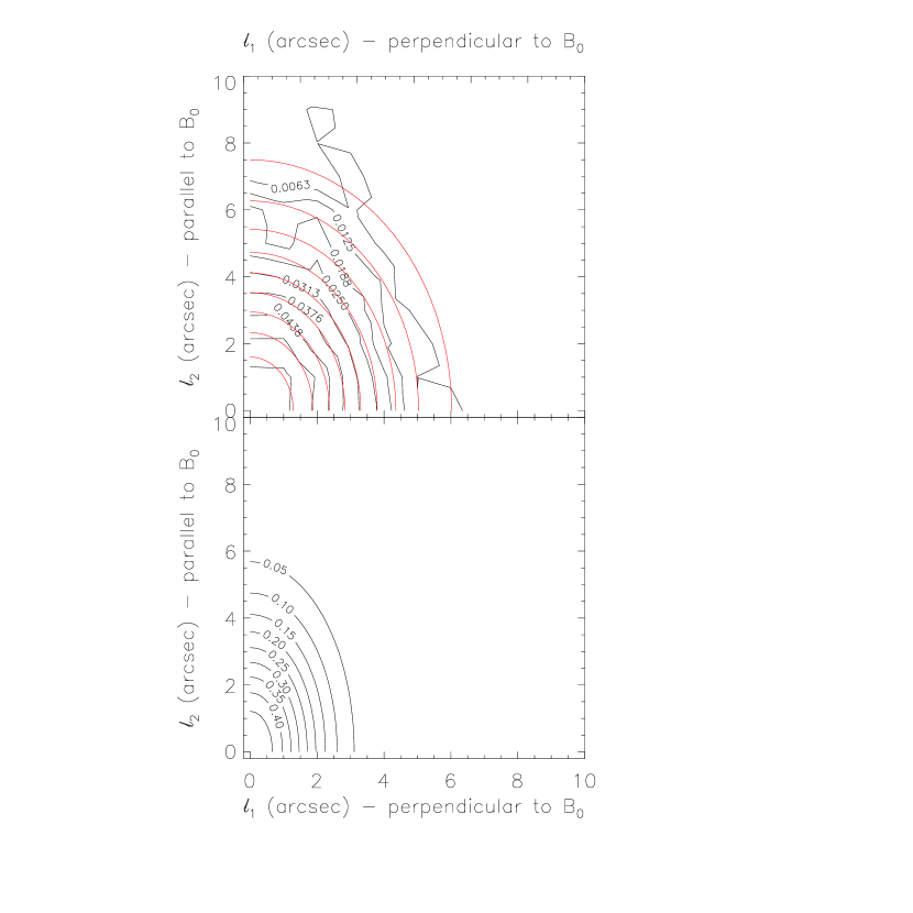
Figure 13: Top: contour plot of the two-dimensional turbulence autocorrelation function (black) and a Gaussian fit (red); the fit is forced to be even in directions parallel and perpendicular to the mean magnetic field. The contours are drawn at 10 to 90 percent (10 percent increments) of the peak $b^{2}\left(0\right)=0.063$. Bottom: the intrinsic turbulence autocorrelation function, where we set $W=0$, $\alpha=\pi/2$, and $N=1$ in Equations (19) and (21), while using the values for $\delta_{\|}$ and $\delta_{\bot}$ obtained with the Gaussian fit (red) in the plot on the top graph (see Table 3). The contours are drawn at 10 to 90 percent (10 percent increments) of the peak $\left\langle B_{\mathrm{t}}^{2}\right\rangle/\left\langle B^{2}\right\rangle=0.50$.

Table 3: Results for two-dimensional anisotropic turbulence ($\alpha=70^{\circ}$).

	All regions
$\delta_{\parallel}$ (pc)	$98\pm 5$
$\delta_{\perp}$ (pc)	$54\pm 3$
$\delta_{\parallel}/\delta_{\perp}$	$1.83\pm 0.13$
$N$	$15\pm 2$
$\left\langle\overline{B}_{\mathrm{t}}^{2}\right\rangle/\left\langle\overline{B}^{2}\right\rangle$	$0.063\pm 0.008$
$\left\langle B_{\mathrm{t}}^{2}\right\rangle/\left\langle B_{0}^{2}\right\rangle$	$1.02\pm 0.08$
$B_{\mathrm{t}}/B_{0}$	$1.01\pm 0.04$

5 Discussion

Our application of the dispersion analysis of Hildebrand et al. (2009) and Houde et al. (2009, 2011), and its generalization to include anisotropy, to M51 reveals some interesting information on the nature of magnetized turbulence in this galaxy. As was previously mentioned, it is important to note that both our analysis and that of Fletcher et al. (2011) yield results that are consistent with one another, even though they are based on completely different approaches. For example, Fletcher et al. (2011) determined the size of a turbulent cell (i.e., approximately twice the turbulent correlation length) by using their measured dispersion of rotation measure, while accounting for the averaging of turbulence inherent to the observation process (see their Equations (3) and (5)). Their value of approximately $50$ pc for the size of a turbulent cell can be readily compared with our estimates of $\delta\simeq 65$ pc determined for isotropic turbulence in Section 4.1 (see Table 1). It is noteworthy that both techniques provide results that are within a factor of two or so from each other, which is interesting considering the uncertainty in the adopted values for some parameters (e.g., the mean electron density $\left\langle n_{\mathrm{e}}\right\rangle=0.1$ cm^-3 used in their calculations).

Fletcher et al. (2011) were also able to discern between the contribution of the different components of the total magnetic field. They found that the total magnetic field $B\sim 15\,\mu\mathrm{G}$ is split into an ordered ($B_{0}$) and an isotropic (i.e., random, $B_{\mathrm{t}}$) components each of $\sim 10\,\mu\mathrm{G}$. It is important to note that their definition of an “ordered” magnetic field is not restricted to a “mean” field, which would result from the average of the magnetic field vector over some suitable (large) scale. More precisely, they define the ordered field as that which is traced by the polarized emission. For M51 they find that the ordered magnetic field is composed of a weak $\sim 2\,\mu\mathrm{G}$ mean component and an anisotropic random field of $\sim 10\,\mu\mathrm{G}$ (we note that such a “mean component” implies a field with a coherent direction, while the anisotropic field has reversing directions). This anisotropic field, presumably resulting from “compression in the spiral arms or localized enhanced shear,” would then display a stronger azimuthal variation and thus be responsible for most of the polarized radio emission in M51 (Fletcher et al., 2011). Their analysis therefore yields $B_{\mathrm{t}}/B_{0}\simeq 1$, as was mentioned earlier. Since our dispersion analysis is based on changes in the orientation of polarization vectors with length scale, it will not be able to discriminate between anisotropic random and mean field components of the ordered field and we cannot comment on its detailed nature. We note, however, that our estimates $B_{\mathrm{t}}/B_{0}\simeq 1.13$ and $1.04$ determined for the isotropic turbulence case in Section 4.1 are in excellent agreement with that of Fletcher et al. (2011) (see Table 1). The typical degrees of polarization, at $\lambda 6\>\mathrm{cm}$ and $4\arcsec$ resolution, in the three regions that we consider are $p=34\%$ in the northeast arm, $p=29\%$ in the southwest arm, and $p=15\%$ in the centre: in calculating these values we have assumed that $25\%$ of the continuum emission at $\lambda 6\>\mathrm{cm}$ is thermal (Fletcher et al., 2011). For the arms these data are in good agreement with the degree of polarization expected when $B_{t}/B_{0}\approx 1$, as $p=0.7\>B_{0}^{2}/(B_{0}^{2}+B_{t}^{2})\approx 0.35$. This shows that the estimates of $B_{t}/B_{0}$ derived from our polarization angle dispersion analysis are compatible with independent methods of interpreting polarization data. In the centre of M51 the physical environment is different from the rest of the disc, due to the presence of an AGN and jet, and so the fraction of thermal emission and thus the degree of polarization are harder to estimate. In addition, in this region the polarized emission can originate from a different location than a large fraction of the total synchrotron emission, again making a useful estimate of $p$ difficult.

Perhaps the most important result stemming from our analysis is the clear detection of anisotropy in the magnetized turbulence. Whether we consider the three analyzable regions of M51 separately or together we consistently find that the turbulent correlation length is larger in a direction parallel to the mean orientation of the local magnetic field than in a direction perpendicular to it (see Tables 2 and 3). As was mentioned in Section 4.2, this result is predicted by current theories for incompressible and compressible MHD turbulence (Goldreich & Sridhar, 1995; Cho, Lazarian, & Vishniac, 2002; Cho & Lazarian, 2003; Kowal & Lazarian, 2010). Such anisotropy has also been observed in the Taurus (Heyer et al., 2008) and Orion molecular clouds (Chitsazzadeh et al., 2012) within our Galaxy. The level of anisotropy we observe in M51, which we quantify with the parallel-to-perpendicular correlation length ratio $\delta_{\|}/\delta_{\bot}$, is significant and in qualitative agreement with numerical simulations of magnetized turbulence. Our contour plot of the turbulent autocorrelation function (see the bottom panel of Figure 13) can be compared with the simulations of incompressible MHD turbulence of Cho, Lazarian, & Vishniac (2002), for example. In particular, the turbulent velocity correlation function presented in their Figure 6 has an appearance that is similar to our derived intrinsic two-dimensional magnetized turbulence autocorrelation function. We would expect such similarities between these two types of autocorrelation functions under the flux-freezing approximation, which should hold in the medium probed with synchrotron polarization observations. Our clearest measure of anisotropy uses the more comprehensive Gaussian model defined with Equations (19) to (21), where the polarization data were analyzed for M51 as a whole without discriminating between the different regions. The significant amount of anisotropy thus measured, with $\delta_{\|}/\delta_{\bot}\simeq 1.8$, is a statement of the importance of magnetic fields on the dynamics of the gas probed by the observations. We should also note that this anisotropy of the magnetized turbulent autocorrelation function is different from that discussed by Fletcher et al. (2011), which pertains to the relative intensity of the two orthogonal components of the random magnetic field. Our analysis cannot say anything concerning any such anisotropy in the field strength, it can only inform us on the relative turbulent energy contained in the magnetic field through measurements of $\left\langle B_{\mathrm{t}}^{2}\right\rangle/\left\langle B_{0}^{2}\right\rangle$, for example.

5.1 Shortcomings of the Dispersion Analysis

Although the quality of the data and the high resolution with which they were obtained allowed us to determine some fundamental parameters that characterize magnetized turbulence in M51, we expect that a slightly higher resolution and sampling rate would result in an even more exhaustive analysis. As was shown by Houde et al. (2011) using submillimeter dust polarization data for Galactic molecular clouds, spatial resolutions resulting in smaller telescope beams such that $\delta\gtrsim\sqrt{2}W$ not only allow the determination of the same parameters uncovered by the present analysis, they can also potentially reveal the underlying turbulent power spectrum. This is because the beam-broadened turbulent autocorrelation function $b^{2}\left(\boldsymbol{\ell}\right)$ is related to the turbulent power spectrum $b^{2}\left(\mathbf{k}_{v}\right)$ through a simple Fourier transform. It is then found that

$$b^{2}\left(\mathbf{k}_{v}\right)=\frac{1}{\left\langle\overline{B}^{2}\right\rangle}\left\|H\left(\mathbf{k}_{v}\right)\right\|^{2}\left[\frac{1}{2\pi}\int\mathcal{R}_{\mathrm{t}}\left(\mathbf{k}_{v},k_{u}\right)\mathrm{sinc}^{2}\left(\frac{k_{u}\Delta}{2}\right)dk_{u}\right],$$ (29)

with $\mathcal{R}_{\mathrm{t}}\left(\mathbf{k}_{v},k_{u}\right)$ and $H\left(\mathbf{k}_{v}\right)$ the Fourier transforms of the intrinsic turbulent autocorrelation function (i.e., not beam-broadened) and the telescope beam, respectively (see the Appendix, and Houde et al. 2011 for a detailed discussion). It follows that beams of smaller spatial extent than the intrinsic turbulent autocorrelation function will have a broader spectral coverage that will reduce their filtering effect on the power spectrum. It then becomes possible to effectively invert Equation (29) to reveal the underlying power spectrum (through some “deconvolution” techniques, for example). In such cases, it is not necessary to assume any model for the turbulence, such as the Gaussian form used in our analysis. The measured turbulent power spectrum could thus be modeled directly from the data and compared to candidate theories for magnetized turbulence.

As can be seen from our results for $b^{2}\left(\boldsymbol{\ell}\right)$ in Figures 4-6, 8-10, and 12, however, the contribution of the correlation length to the width of the beam-broadened turbulent autocorrelation function (approximately gauged through the ratio $\delta^{2}/\left(\delta^{2}+2W^{2}\right)$; see Equations (20) and (23)) is typically modest, implying that the spectral filtering of the telescope beam is too severe to recover the intrinsic turbulent power spectrum. But even a relatively modest increase in spatial resolution, e.g., by a factor of a few, could allows us to recover the power spectrum in future observations.

Another negative impact of a larger telescope beam and its broadening of the autocorrelation function $b^{2}\left(\boldsymbol{\ell}\right)$ is that it renders more difficult the separation of the small and large scale components present in the dispersion function. For M51 this means that the scale of the turbulence, quantified with $\delta$, can get “mixed up” with the larger scale of the spiral structure through its artificial broadening to $\delta^{2}+2W^{2}$ caused by the beam. As alluded to in Section 4.1, this may be a reason why we were unable to see any contribution from $\delta$ to the width of $b^{2}\left(\boldsymbol{\ell}\right)$ in our analyses of the northeast arm (see Figs. 4 and 8). More precisely, we were unable to cleanly separate the large from the small scale using our Taylor expansions, i.e., Equations (16) and (24). This is probably also true, but to a lesser extent, for the other two regions studied, as can be seen from the absence of significant “tails” for $\ell\gtrsim 5\arcsec$ in $b^{2}\left(\boldsymbol{\ell}\right)$. An increase in spatial resolution would resolve this issue, which is likely to bring some error in our determination of the correlation length scales and turbulent to total energy ratios. We expect this error to be small, but it is not possible to quantify it at this point.

Finally, we wish to once again emphasize that the choice of a Gaussian turbulence model is unlikely to be realistic for M51. But in view of the aforementioned impossibility to uncover the underlying turbulent power spectrum because of the significant spectral beam filtering, this model, which can be solved analytically, allows us to quantify key parameters that characterize magnetized turbulence. Furthermore, our more comprehensive model for anisotropic Gaussian turbulence defined with Equations (19) and (20) implicitly assumes that the $N$ ellipsoid turbulent cells contained in the column of gas probed by the telescope beam have the same spatial orientation in relation to the local magnetic field. This is clearly unlikely to be true across the beam ($\mathrm{FWHM}\simeq 148$ pc), or through the thickness ($\sim 800$ pc) and the extent of the studied regions on the galactic disk. It is therefore more realistic to view the correlation lengths $\delta_{\|}$ and $\delta_{\bot}$ as some averages representative for magnetized turbulence in M51.

6 Summary

We conducted a dispersion analysis, using a generalization of the technique of Houde et al. (2009) to previously published high-resolution synchrotron polarization data (Fletcher et al., 2011) with the goal of charactering magnetized turbulence in M51. We first analyzed three distinct regions (the center of the galaxy, and the northwest and southwest spiral arms) and measured the turbulent correlation length scale from the width of the magnetized turbulent correlation function for two regions and detected the imprint of anisotropy in the turbulence for all three. Furthermore, analyzing the galaxy as a whole allowed us to determine a two-dimensional Gaussian model for the magnetized turbulence in M51. We measured the turbulent correlation scales along and perpendicular to the local mean magnetic field to be, respectively, $\delta_{\|}=98\pm 5$ pc and $\delta_{\bot}=54\pm 3$ pc, while the turbulent to ordered magnetic field strength ratio is found to be $B_{\mathrm{t}}/B_{0}=1.01\pm 0.04$. These results are in agreement with those of Fletcher et al. (2011), who performed a Faraday rotation dispersion analysis of the same data. Finally, our detection of anisotropy, quantified with a parallel-to-perpendicular correlation length ratio with $\delta_{\|}/\delta_{\bot}\simeq 1.83\pm 0.13$, is consistent with current magnetized turbulence theories.

Appendix A Anisotropic Gaussian Magnetized Turbulence

The cloud- and beam-integrated magnetic field is defined with

$$\overline{\mathbf{B}}\left(\mathbf{r}\right)=\iint H\left(\mathbf{r}-\mathbf{a}\right)\left[\frac{1}{\Delta}\int_{0}^{\Delta}F_{0}\left(\mathbf{a},z\right)\mathbf{B}\left(\mathbf{a},z\right)dz\right]d^{2}a,$$ (A1)

where the beam profile is denoted by $H\left(\mathbf{r}\right)$, while the weighting function $F_{0}\left(\mathbf{a},z\right)\geq 0$ is the (ordered) polarized emission associated with the magnetic field $\mathbf{B}\left(\mathbf{a},z\right)$, and $\Delta$ is the maximum depth of the cloud along any line of sight. The integrated autocorrelation function is then

$$\left\langle\overline{\mathbf{B}}_{\mathrm{t}}\mathbf{\cdot}\overline{\mathbf{B}}_{\mathrm{t}}\mathbf{\left(\boldsymbol{\ell}\right)}\right\rangle=\iint\iint H\left(\mathbf{a}\right)H\left(\mathbf{a}^{\prime}+\boldsymbol{\ell}\right)\left[\frac{2}{\Delta}\int_{0}^{\Delta}\left(1-\frac{u}{\Delta}\right)\mathcal{R}_{\mathrm{t}}\left(\mathbf{v},u\right)du\right]d^{2}a^{\prime}d^{2}a,$$ (A2)

with $\mathcal{R}_{\mathrm{t}}\left(v,u\right)=\left\langle F_{0}\left(\mathbf{a},z\right)F_{0}\left(\mathbf{a}^{\prime},z^{\prime}\right)\right\rangle\left\langle\mathbf{B}_{\mathrm{t}}\left(\mathbf{a},z\right)\cdot\mathbf{B}_{\mathrm{t}}\left(\mathbf{a}^{\prime},z^{\prime}\right)\right\rangle$, $u=\left|z^{\prime}-z\right|$, and $\mathbf{v}=\mathbf{a}^{\prime}-\mathbf{a}$ ($\equiv v_{1}\mathbf{e}_{1}+v_{2}\mathbf{e}_{2}$; Houde et al. 2009). We refer to $\left(v_{1},v_{2},u\right)$ as the observer coordinate system, the $v_{1}$ and $v_{2}$ axes define the plane of the sky, while the line of sight point along the negative $u$-axis.

The assumptions of statistical independence between the turbulent and ordered magnetic fields, homogeneity in their strength across the source, and of overall stationarity previously stated in Section 2.2 are all required to arrive at Equations (A1) and (A2). Of these, the assumption of homogeneity is particularly useful for analyzing our data. This is because synchrotron polarization signals bring in the complication that the weighting function $F_{0}\left(\mathbf{a},z\right)$ is also a function of the magnetic field strength (approximately proportional to its second power), and would therefore appear to significantly jeopardize any calculations stemming form Equation (A2). However, this dependency is seen to disappear in the calculation of the angular dispersion function (Equation (10)) when homogeneity is assumed, since this weighting function will have the same proportionality factor (due to the field strength) at all points in the source (i.e., in the integrands of Equations (A1) and (A2)). Our analysis can then proceed in a manner similar to the simpler case of polarization dust emission signals, where there is no linked between the value of $F_{0}\left(\mathbf{a},z\right)$ and the strength of the magnetic field (Houde et al., 2009).

In cases where the autocorrelation function for anisotropic magnetized turbulence is idealized with a Gaussian ellipsoid we write

$$R_{\mathrm{t}}\left(\boldsymbol{\xi},\tau\right) = \left\langle F_{0}^{2}\left(\boldsymbol{\xi},\tau\right)\right\rangle\left\langle B_{\mathrm{t}}^{2}\right\rangle e^{-\frac{1}{2}\left(\tau^{2}/\delta_{\|}^{2}+\xi^{2}/\delta_{\bot}^{2}\right)}$$ (A3)

$$\simeq \left\langle F_{0}^{2}\right\rangle\left\langle B_{\mathrm{t}}^{2}\right\rangle e^{-\frac{1}{2}\left(\tau^{2}/\delta_{\|}^{2}+\xi^{2}/\delta_{\bot}^{2}\right)},$$

where $\boldsymbol{\xi}$ ($=\left(\xi_{1},\xi_{2}\right)$) is a two-dimensional displacement vector perpendicular to the orientation of the local ordered magnetic field $\mathbf{B}_{0}$ and $\tau$ is the displacement along $\mathbf{B}_{0}$; a prolate example is shown in Figure 3 along with the relationship between the $\left(v_{1},v_{2},u\right)$ and $\left(\xi_{1},\xi_{2},\tau\right)$ coordinate systems. We adopt a model for anisotropic magnetized turbulence where the symmetry axis of the ellipsoid is aligned with $\mathbf{B}_{0}$; this also implies that the length scale of the ordered field is much larger than the correlation lengths $\delta_{\|}$ and $\delta_{\bot}$ characterizing the turbulent field $\mathbf{B}_{\mathrm{t}}$. The function $\left\langle F_{0}^{2}\left(\boldsymbol{\xi},\tau\right)\right\rangle$ is the autocorrelation of the ordered polarized emission, which we approximate to a constant $\left\langle F_{0}^{2}\right\rangle\equiv\left\langle F_{0}^{2}\left(\boldsymbol{0},0\right)\right\rangle$ in Equation (A3) as it is assumed that its correlation length is also significantly larger than $\delta_{\|}$ and $\delta_{\bot}$. We seek to express this function (i.e., Equation (A3)) using the observer coordinates $\left(v_{1},v_{2},u\right)$. Referring to Figure 3, the inclination angle relative to the line of sight of the ellipsoid symmetry axis (and of $\mathbf{B}_{0}$) is given by $\alpha$, while the angle $\beta$ defines the orientation of its projection on the plane of the sky. The precise relationship between the two coordinate systems is

$$\xi_{1} = v_{1}\cos\left(\beta\right)+v_{2}\sin\left(\beta\right)$$

$$\xi_{2} = -v_{1}\cos\left(\alpha\right)\sin\left(\beta\right)+v_{2}\cos\left(\alpha\right)\cos\left(\beta\right)+u\sin\left(\alpha\right)$$ (A4)

$$\tau = v_{1}\sin\left(\alpha\right)\sin\left(\beta\right)-v_{2}\sin\left(\alpha\right)\cos\left(\beta\right)+u\cos\left(\alpha\right),$$

such that

$$\frac{\tau^{2}}{\delta_{\|}^{2}}+\frac{\xi^{2}}{\delta_{\bot}^{2}}=\frac{u^{2}}{\eta^{2}}+\frac{v_{1}^{2}}{\kappa_{1}^{2}}+\frac{v_{2}^{2}}{\kappa_{2}^{2}}-\frac{2}{\kappa_{12}^{2}}v_{1}v_{2}+\frac{2}{\sigma_{1}^{2}}uv_{1}-\frac{2}{\sigma_{2}^{2}}uv_{2},$$ (A5)

with

$$\frac{1}{\eta^{2}} = \frac{\cos^{2}\left(\alpha\right)}{\delta_{\|}^{2}}+\frac{\sin^{2}\left(\alpha\right)}{\delta_{\bot}^{2}}$$

$$\frac{1}{\sigma_{1}^{2}} = \left(\frac{1}{\delta_{\|}^{2}}-\frac{1}{\delta_{\bot}^{2}}\right)\sin\left(\alpha\right)\cos\left(\alpha\right)\sin\left(\beta\right)$$

$$\frac{1}{\sigma_{2}^{2}} = \left(\frac{1}{\delta_{\|}^{2}}-\frac{1}{\delta_{\bot}^{2}}\right)\sin\left(\alpha\right)\cos\left(\alpha\right)\cos\left(\beta\right)$$

$$\frac{1}{\kappa_{1}^{2}} = \frac{\sin^{2}\left(\alpha\right)\sin^{2}\left(\beta\right)}{\delta_{\|}^{2}}+\frac{\cos^{2}\left(\beta\right)+\cos^{2}\left(\alpha\right)\sin^{2}\left(\beta\right)}{\delta_{\bot}^{2}}$$ (A6)

$$\frac{1}{\kappa_{2}^{2}} = \frac{\sin^{2}\left(\alpha\right)\cos^{2}\left(\beta\right)}{\delta_{\|}^{2}}+\frac{\sin^{2}\left(\beta\right)+\cos^{2}\left(\alpha\right)\cos^{2}\left(\beta\right)}{\delta_{\bot}^{2}}$$

$$\frac{1}{\kappa_{12}^{2}} = \left(\frac{1}{\delta_{\|}^{2}}-\frac{1}{\delta_{\bot}^{2}}\right)\sin^{2}\left(\alpha\right)\sin\left(\beta\right)\cos\left(\beta\right).$$

Inserting Equations (A5) and (A6) in Equation (A3) we can express the turbulent autocorrelation function with a dependency on $\left(v_{1},v_{2},u\right)$.

It is advantageous to solve Equation (A2) by considering its Fourier transform (i.e., the turbulent power spectrum; Houde et al. 2009, 2011)

$$\overline{B}_{\mathrm{t}}^{2}\left(\mathbf{k}_{v}\right)=\left\|H\left(\mathbf{k}_{v}\right)\right\|^{2}\left[\frac{1}{2\pi}\int\mathcal{R}_{\mathrm{t}}\left(\mathbf{k}_{v},k_{u}\right)\mathrm{sinc}^{2}\left(\frac{k_{u}\Delta}{2}\right)dk_{u}\right],$$ (A7)

with the correspondence $\left(\mathbf{v},u\right)\rightleftharpoons\left(\mathbf{k}_{v},k_{u}\right)$ between the two domains, and then recover the autocorrelation function through the inverse Fourier transform

$$\left\langle\overline{\mathbf{B}}_{\mathrm{t}}\mathbf{\cdot}\overline{\mathbf{B}}_{\mathrm{t}}\mathbf{\left(\boldsymbol{\ell}\right)}\right\rangle=\frac{1}{\left(2\pi\right)^{2}}\iint\overline{B}_{\mathrm{t}}^{2}\left(\mathbf{k}_{v}\right)e^{i\mathbf{k}_{v}\cdot\boldsymbol{\ell}}d^{2}k_{v}.$$ (A8)

We note that the two-dimensional power spectrum given by Equation (A7) could be compared to a Kolmogorov-type spectrum, for example, by first multiplying it by $2\pi k_{v}$ (for a three-dimensional spectrum a factor of $4\pi k_{v}^{2}$ would be required; see Houde et al. 2009, 2011).

The solution for this problem mostly rests on the repeated application of the following relation for the integration of Gaussian functions

$$\int_{-\infty}^{\infty}e^{-\left(a^{2}x^{2}+bx\right)}dx=\frac{\sqrt{\pi}}{a}e^{\left(b/2a\right)^{2}},$$ (A9)

with $a$ and $b$ some constants. Considering Equation (A9) and the fact that the Fourier transform of a rotated function equals the rotated version of the Fourier transform of the unrotated function (i.e., when $\alpha=\beta=0$; see Appendix 4 of Houde & Vaillancourt 2007), the Fourier transform of the turbulent autocorrelation function can be calculated to be

$$\mathcal{R}_{\mathrm{t}}\left(\mathbf{k}_{v},k_{u}\right)=\left\langle F_{0}^{2}\right\rangle\left\langle B_{\mathrm{t}}^{2}\right\rangle\left(2\pi\right)^{3/2}\delta_{\|}\delta_{\bot}^{2}e^{-\frac{1}{2}\left(\epsilon^{2}k_{u}^{2}+\mu_{1}^{2}k_{1}^{2}+\mu_{2}^{2}k_{2}^{2}-2\mu_{12}^{2}k_{1}k_{2}+2\gamma_{1}^{2}k_{u}k_{1}-2\gamma_{2}^{2}k_{u}k_{2}\right)}$$ (A10)

with

$$\epsilon^{2} = \delta_{\|}^{2}\cos^{2}\left(\alpha\right)+\delta_{\bot}^{2}\sin^{2}\left(\alpha\right)$$

$$\gamma_{1}^{2} = \left(\delta_{\|}^{2}-\delta_{\bot}^{2}\right)\sin\left(\alpha\right)\cos\left(\alpha\right)\sin\left(\beta\right)$$

$$\gamma_{2}^{2} = \left(\delta_{\|}^{2}-\delta_{\bot}^{2}\right)\sin\left(\alpha\right)\cos\left(\alpha\right)\cos\left(\beta\right)$$

$$\mu_{1}^{2} = \delta_{\|}^{2}\sin^{2}\left(\alpha\right)\sin^{2}\left(\beta\right)+\delta_{\bot}^{2}\left[\cos^{2}\left(\beta\right)+\cos^{2}\left(\alpha\right)\sin^{2}\left(\beta\right)\right]$$ (A11)

$$\mu_{2}^{2} = \delta_{\|}^{2}\sin^{2}\left(\alpha\right)\cos^{2}\left(\beta\right)+\delta_{\bot}^{2}\left[\sin^{2}\left(\beta\right)+\cos^{2}\left(\alpha\right)\cos^{2}\left(\beta\right)\right]$$

$$\mu_{12}^{2} = \left(\delta_{\|}^{2}-\delta_{\bot}^{2}\right)\sin^{2}\left(\alpha\right)\sin\left(\beta\right)\cos\left(\beta\right)$$

and $\mathbf{k}_{v}\equiv k_{1}\mathbf{e}_{1}+k_{2}\mathbf{e}_{2}$.

We also note that because the depth of integration along the line of sight is expected to be much larger then the turbulent correlation lengths (i.e., $\Delta\gg\delta_{\|}$ and $\Delta\gg\delta_{\bot}$) we have

$$\int e^{-\frac{1}{2}\left(\epsilon^{2}k_{u}^{2}+2\gamma_{1}^{2}k_{u}k_{1}-2\gamma_{2}^{2}k_{u}k_{2}\right)}\mathrm{sinc}^{2}\left(\frac{k_{u}\Delta}{2}\right)dk_{u} \simeq \int\mathrm{sinc}^{2}\left(\frac{k_{u}\Delta}{2}\right)dk_{u}$$ (A12)

$$\simeq \frac{2\pi}{\Delta}.$$

Inserting Equation (A12) in Equation (A7) with

$$H\left(\mathbf{k}_{v}\right)=e^{-\frac{1}{2}W^{2}k_{v}^{2}},$$ (A13)

and further using Equation (A9), it is found that

$$\overline{B}_{\mathrm{t}}^{2}\left(\mathbf{k}_{v}\right)=\left\langle F_{0}^{2}\right\rangle\left\langle B_{\mathrm{t}}^{2}\right\rangle\left(2\pi\right)^{3/2}\frac{\delta_{\|}\delta_{\bot}^{2}}{\Delta}e^{-\frac{1}{2}\left[k_{1}^{2}\left(\mu_{1}^{2}+2W^{2}\right)+k_{2}^{2}\left(\mu_{2}^{2}+2W^{2}\right)-2\mu_{12}^{2}k_{1}k_{2}\right]}.$$ (A14)

Calculating the inverse Fourier transform of Equation (A14), still using Equation (A9), then yields

$$\left\langle\overline{\mathbf{B}}_{\mathrm{t}}\mathbf{\cdot}\overline{\mathbf{B}}_{\mathrm{t}}\mathbf{\left(\boldsymbol{\ell}\right)}\right\rangle=\frac{\left\langle F_{0}^{2}\right\rangle\left\langle B_{\mathrm{t}}^{2}\right\rangle}{N^{\prime}}e^{-\frac{1}{2}g\left(\boldsymbol{\ell};\delta_{\|},\delta_{\bot};\alpha,\beta\right)},$$ (A15)

with

$$g\left(\boldsymbol{\ell};\delta_{\|},\delta_{\bot};\alpha,\beta\right) = \left[\ell_{1}+\mu_{12}^{2}\ell_{2}/\left(\mu_{2}^{2}+2W^{2}\right)\right]^{2}/\left[\mu_{1}^{2}+\mu_{12}^{4}/\left(\mu_{2}^{2}+2W^{2}\right)+2W^{2}\right]$$ (A16)

$$+\ell_{2}^{2}/\left(\mu_{2}^{2}+2W^{2}\right)$$

and

$$\frac{1}{N^{\prime}}=\frac{\sqrt{2\pi}\delta_{\|}\delta_{\bot}^{2}}{\sqrt{\left[\mu_{1}^{2}+\mu_{12}^{4}/\left(\mu_{2}^{2}+2W^{2}\right)+2W^{2}\right]\left(\mu_{2}^{2}+2W^{2}\right)}\,\Delta}.$$ (A17)

Following the treatment of Houde et al. (2009) for the ordered component of the autocorrelation function we write

$$\left\langle\overline{B}_{0}^{2}\right\rangle\equiv\left\langle F_{0}^{2}\right\rangle\left\langle B_{0}^{2}\right\rangle\frac{\Delta^{\prime}}{\Delta},$$ (A18)

where $\Delta^{\prime}\leq\Delta$ is the effective depth over which the signal is integrated along the line of sight (in our case approximately the thickness of the disk of M51), which is closely related to the correlation length of the ordered polarized flux (see Secs. 2.3 and 3.2 in Houde et al. 2009).

Combining Equations (A15)-(A18) we find

$$b^{2}\left(\boldsymbol{\ell}\right) = \frac{\left\langle\overline{\mathbf{B}}_{\mathrm{t}}\mathbf{\cdot}\overline{\mathbf{B}}_{\mathrm{t}}\left(\boldsymbol{\ell}\right)\right\rangle}{\left\langle\overline{\mathbf{B}}\mathbf{\cdot}\overline{\mathbf{B}}\left(0\right)\right\rangle}$$ (A19)

$$= \left[\frac{\left\langle B_{\mathrm{t}}^{2}\right\rangle}{N\left\langle B_{0}^{2}\right\rangle+\left\langle B_{\mathrm{t}}^{2}\right\rangle}\right]e^{-\frac{1}{2}g\left(\boldsymbol{\ell};\delta_{\|},\delta_{\bot};\alpha,\beta\right)}$$

with the number of turbulent cells $N$ probed by the telescope beam given by

$$\frac{1}{N}=\frac{\sqrt{2\pi}\delta_{\|}\delta_{\bot}^{2}}{\sqrt{\left[\mu_{1}^{2}+\mu_{12}^{4}/\left(\mu_{2}^{2}+2W^{2}\right)+2W^{2}\right]\left(\mu_{2}^{2}+2W^{2}\right)}\,\Delta^{\prime}}.$$ (A20)

If we choose to align one of the axes of the observer’s coordinate system on the plane of the sky (i.e., the $v_{2}$-axis) with the large scale magnetic field $\mathbf{B}_{0}$, then $\beta=0$ and Equations (A19) and (A20) reduce to Equations (19) and (20), respectively.

References

- Beck et al. (2005) Beck, R., Fletcher, A., Shukurov, A., Snodin, A., Sokoloff, D. D., Ehle, M., Moss, D., and Shoutenkov, V. 2005, A&A, 444, 739
- Beck et al. (1999) Beck, R., Berkhuijsen, E. M., and Uyanıker, B. 1999, in Plasma Turbulence and Energetic Particles in Astrophysics, eds. M. Otrowski and R. Schlickeiser (Kraków: Obs. Astron. Univ. Jagiellongski), 5
- Brown & Taylor (2001) Brown, J. C. and Taylor, A. R. 2001, ApJ, 563, L31
- Chitsazzadeh et al. (2012) Chitsazzadeh, S., Houde, M., Hildebrand, R. H., and Vaillancourt, J. E. 2012, ApJ, 749, 45
- Cho, Lazarian, & Vishniac (2002) Cho, J., Lazarian, A., and Vishniac, E. T. 2002, ApJ, 564, 291
- Cho & Lazarian (2003) Cho, J., & Lazarian, A. 2003, MNRAS, 345, 325
- Ciardullo et al. (2002) Ciardullo, R., Feldmeier, J. J., Jacoby, G. H., et al. 2002, ApJ, 577, 31
- Falceta-Gonçalves et al. (2008) Falceta-Gonçalves, D., Lazarian, A., & Kowal, G. 2008, ApJ, 679, 537
- Fletcher et al. (2011) Fletcher, A., Beck, R., Shukurov, A., Berkhuijsen, E. M., and Horellou, C. 2011, MNRAS, 412, 2396
- Frisch (1995) Frisch, U. 1995, Turbulence: The Legacy of A. N. Kolmogorov (Cambridge: Cambridge Univ. Press)
- Goldreich & Sridhar (1995) Goldreich, P. and Sridhar, S. 1995, ApJ, 438, 763
- Heyer et al. (2008) Heyer, M., Gong, H., Ostriker, E., and Brunt, C. 2008, ApJ, 680, 420
- Hildebrand et al. (2009) Hildebrand, R. H., Kirby, L., Dotson, J. L., Houde, M., and Vaillancourt, J. E. 2009, ApJ, 696, 567
- Houde & Vaillancourt (2007) Houde, M. and Vaillancourt, J. E. 2007, PASP, 119, 871
- Houde et al. (2009) Houde, M., Vaillancourt, J. E., Hildebrand, R. H., Chitsazzadeh, S., and Kirby, L. 2009, ApJ, 706, 1504
- Houde et al. (2011) Houde, M., Rao, R., Vaillancourt, J. E., & Hildebrand, R. H., 2011, ApJ, 733, 109
- Jaffe et al. (2010) Jaffe, T. R., Leahy, J. P., Banday, A. J., Leach, S. M., Lowe and Wilkinson, W. 2010, MNRAS, 401, 1013
- Jansson & Farrar (2012) Jansson, R. and Farrar, G. R. 2012, arXiv:1204.3662
- Kowal & Lazarian (2010) Kowal, G., & Lazarian, A. 2010, ApJ, 720, 742
- Tully (1974) Tully, R. B. 1974, ApJS, 27, 437
- Wardle & Kronberg (1974) Warner, J. F. C., & Kronberg, P. P. 1974, ApJ, 194, 249