Optimal dividends in the dual model under transaction costs

Abstract.

We analyze the optimal dividend payment problem in the dual model under constant transaction costs. We show, for a general spectrally positive Lévy process, an optimal strategy is given by a $(c_{1},c_{2})$-policy that brings the surplus process down to $c_{1}$ whenever it reaches or exceeds $c_{2}$ for some $0\leq c_{1}<c_{2}$. The value function is succinctly expressed in terms of the scale function. A series of numerical examples are provided to confirm the analytical results and to demonstrate the convergence to the no-transaction cost case, which was recently solved by Bayraktar et al. [8].
Key words: dual model; dividends; impulse control; spectrally positive Lévy processes; scale functions.
JEL Classification: C44, C61, G24, G32, G35
AMS 2010 Subject Classifications: 60G51, 93E20

1. Introduction

We solve the optimal dividend problem under fixed transaction costs in the so-called dual model, in which the surplus of a company is driven by a Lévy process with positive jumps (spectrally positive Lévy process). This is an appropriate model for a company driven by inventions or discoveries. The case without transaction costs has recently been well-studied; see [3], [7], [2], and [4]. In particular, in [8], we show the optimality of a barrier strategy (reflected Lévy process) for a general spectrally positive Lévy process of bounded or unbounded variation.

A strategy is assumed to be in the form of impulse control; whenever dividends are accrued, a constant transaction cost $\beta>0$ is incurred. As opposed to the barrier strategy that is typically optimal for the no-transaction cost case, we shall pursue the optimality of the so-called $(c_{1},c_{2})$-policy that brings the surplus process down to $c_{1}$ whenever it reaches or exceeds $c_{2}$ for some $0\leq c_{1}<c_{2}<\infty$. While, as in [18, 22], an optimal strategy may not lie in the set of $(c_{1},c_{2})$-policies for the spectrally negative Lévy case, we shall show that it is indeed so in the dual model for any choice of underlying spectrally positive Lévy process. As a related work, we refer the reader to a compound Poisson dual model by [25] where transaction costs are incurred for capital injections. In inventory control, the optimality of similar policies, called $(s,S)$-policies, is shown to be optimal in [9, 10] for a mixture of a Brownian motion and a compound Poisson process and in [24] for a general spectrally negative Lévy process.

Following [8], we take advantage of the fluctuation theory for the spectrally positive Lévy process (see e.g. [11], [13] and [17]). The expected net present value (NPV) of dividends (minus transaction costs) under a $(c_{1},c_{2})$-policy until ruin is first written in terms of the scale function. We then show the existence of the maximizers $0\leq c_{1}^{*}<c_{2}^{*}<\infty$ that satisfy the continuous fit (resp. smooth fit) at $c_{2}^{*}$ when the surplus process is of bounded (resp. unbounded) variation and that the derivative at $c_{1}^{*}$ is one when $c_{1}^{*}>0$ and is less than or equal to one when $c_{1}^{*}=0$. These properties are used to verify the optimality of the $(c_{1}^{*},c_{2}^{*})$-policy.

In order to evaluate the analytical results and to examine the connection with the no-transaction cost case developed by [8], we conduct a series of numerical experiments using Lévy processes with positive i.i.d. phase-type jumps with or without Brownian motion [1]. We shall confirm the existence of the maximizers $0\leq c_{1}^{*}<c_{2}^{*}<\infty$ and examine the shape of the value function at $c_{1}^{*}$ and $c_{2}^{*}$. We further compute for a sequence of unit transaction costs and confirm that, as $\beta\downarrow 0$, the value function as well as $c_{1}^{*}$ and $c_{2}^{*}$ converge to the ones obtained for the no-transaction cost case in [8].

The rest of the paper is organized as follows. Section 2 gives a mathematical model of the problem. In Section 3, we compute the expected NPV of dividends under the $(c_{1},c_{2})$-policy via the scale function. Section 4 shows the existence of $0\leq c_{1}^{*}<c_{2}^{*}<\infty$ that maximize the expected NPV over $c_{1}$ and $c_{2}$. Section 5 verifies the optimality of the $(c_{1}^{*},c_{2}^{*})$-policy. We conclude the paper with numerical results in Section 6.

2. Mathematical Formulation

We will denote the surplus of a company by a spectrally positive Lévy process $X=\left\{X_{t};t\geq 0\right\}$ whose Laplace exponent is given by

(2.1) $$\psi(s):=\log\mathbb{E}\left[e^{-sX_{1}}\right]=cs+\frac{1}{2}\sigma^{2}s^{2}+\int_{(0,\infty)}(e^{-sz}-1+sz1_{\{0<z<1\}})\nu({\rm d}z),\quad s\in\mathbb{R}$$

where $\nu$ is a Lévy measure with the support $(0,\infty)$ that satisfies the integrability condition $\int_{(0,\infty)}(1\wedge z^{2})\nu({\rm d}z)<\infty$. It has paths of bounded variation if and only if $\sigma=0$ and $\int_{(0,1)}z\,\nu({\rm d}z)<\infty$. In this case, we write (2.1) as

$$\psi(s)=\mathfrak{d}s+\int_{(0,\infty)}(e^{-sz}-1)\nu({\rm d}z),\quad s\in\mathbb{R}$$

with $\mathfrak{d}:=c+\int_{(0,1)}z\,\nu({\rm d}z)$; the resulting drift of the process is $-\mathfrak{d}$. We exclude the trivial case in which $X$ is a subordinator (i.e., $X$ has monotone paths a.s.). This assumption implies that $\mathfrak{d}>0$ when $X$ is of bounded variation.

Let $\mathbb{P}_{x}$ be the conditional probability under which $X_{0}=x$ (also let $\mathbb{P}\equiv\mathbb{P}_{0}$), and let $\mathbb{F}:=\left\{\mathcal{F}_{t}:t\geq 0\right\}$ be the filtration generated by $X$. Using this, the drift of $X$ is given by

(2.2) $$\mu:=\mathbb{E}[X_{1}]=-\psi^{\prime}(0+).$$

In order to make sure the problem is non-trivial and well-defined, we assume throughout the paper that this is finite.

Assumption 2.1.

We assume that $\mu\in(-\infty,\infty)$.

A (dividend) strategy $\pi:=\left\{L_{t}^{\pi};t\geq 0\right\}$ is given by a nondecreasing, right-continuous and $\mathbb{F}$-adapted pure jump process starting at zero in the form $L_{t}^{\pi}=\sum_{0\leq s\leq t}\Delta L_{s}^{\pi}$ with $\Delta L_{t}=L_{t}-L_{t-}$, $t\geq 0$. Corresponding to every strategy $\pi$, we associate a controlled surplus process $U^{\pi}=\{U_{t}^{\pi}:t\geq 0\}$, which is defined by

$$U_{t}^{\pi}:=X_{t}-L_{t}^{\pi},\quad t\geq 0,$$

where $U^{\pi}_{0-}=x$ is the initial surplus and $L^{\pi}_{0-}=0$. The time of ruin is defined to be

$$\sigma^{\pi}:=\inf\left\{t>0:U_{t}^{\pi}<0\right\}.$$

A lump-sum payment cannot be more than the available funds and hence it is required that

(2.3) $$\Delta L_{t}^{\pi}\leq U_{t-}^{\pi}+\Delta X_{t},\quad t\leq\sigma^{\pi}\;\;a.s.$$

Let $\Pi$ be the set of all admissible strategies satisfying (2.3). The problem is to compute, for $q>0$, the expected NPV of dividends until ruin

$$v_{\pi}(x):=\mathbb{E}_{x}\Big{[}\int_{0}^{\sigma^{\pi}}e^{-qt}{\rm d}\Big{(}L_{t}^{\pi}-\sum_{0\leq s\leq t}\beta 1_{\{\Delta L_{s}^{\pi}>0\}}\Big{)}\Big{]},\quad x\geq 0,$$

where $\beta>0$ is the unit transaction cost, and to obtain an admissible strategy that maximizes it, if such a strategy exists. Hence the (optimal) value function is written as

(2.4) $$v(x):=\sup_{\pi\in\Pi}v_{\pi}(x),\quad x\geq 0.$$

3. The $(c_{1},c_{2})$-policy

We aim to prove that a $(c_{1}^{*},c_{2}^{*})$-policy is optimal for some $c^{*}_{2}>c_{1}^{*}\geq 0$. For $c_{2}>c_{1}\geq 0$, a $(c_{1},c_{2})$-policy, $\pi_{c_{1},c_{2}}:=\left\{L_{t}^{c_{1},c_{2}};t\geq 0\right\}$, brings the level of the controlled surplus process $U^{c_{1},c_{2}}:=X-L^{c_{1},c_{2}}$ down to $c_{1}$ whenever it reaches or exceeds $c_{2}$. Let us define the corresponding expected NPV of dividends as

(3.1) $$v_{c_{1},c_{2}}(x):=\mathbb{E}_{x}\left[\int_{0}^{\sigma_{c_{1},c_{2}}}e^{-qt}{\rm d}\Big{(}L_{t}^{c_{1},c_{2}}-\sum_{0\leq s\leq t}\beta 1_{\{\Delta L_{s}^{c_{1},c_{2}}>0\}}\Big{)}\right],\quad x\geq 0,$$

where $\sigma_{c_{1},c_{2}}:=\inf\left\{t>0:U_{t}^{c_{1},c_{2}}<0\right\}$ is the corresponding ruin time. In this section, we shall express these in terms of the scale function.

3.1. Scale functions

Fix $q>0$. For any spectrally positive Lévy process, there exists a function called the q-scale function

$$W^{(q)}:\mathbb{R}\rightarrow[0,\infty),$$

which is zero on $(-\infty,0)$, continuous and strictly increasing on $[0,\infty)$, and is characterized by the Laplace transform:

$$\int_{0}^{\infty}e^{-sx}W^{(q)}(x){\rm d}x=\frac{1}{\psi(s)-q},\qquad s>\Phi(q),$$

where

$$\Phi(q):=\sup\{\lambda\geq 0:\psi(\lambda)=q\}.$$

Here, the Laplace exponent $\psi$ in (2.1) is known to be zero at the origin and convex on $[0,\infty)$; therefore $\Phi(q)$ is well-defined and is strictly positive as $q>0$. We also define, for $x\in\mathbb{R}$,

$$\overline{W}^{(q)}(x) :=\int_{0}^{x}W^{(q)}(y){\rm d}y,$$

$$Z^{(q)}(x) :=1+q\overline{W}^{(q)}(x),$$

$$\overline{Z}^{(q)}(x) :=\int_{0}^{x}Z^{(q)}(z){\rm d}z=x+q\int_{0}^{x}\int_{0}^{z}W^{(q)}(w){\rm d}w{\rm d}z.$$

Notice that because $W^{(q)}$ is uniformly zero on the negative half line, we have

(3.2) $$Z^{(q)}(x)=1\quad\textrm{and}\quad\overline{Z}^{(q)}(x)=x,\quad x\leq 0.$$

Let us define the first down- and up-crossing times, respectively, by

(3.3) $$\tau_{a}^{-}:=\inf\left\{t\geq 0:X_{t}<a\right\}\quad\textrm{and}\quad\tau_{b}^{+}:=\inf\left\{t\geq 0:X_{t}>b\right\},\quad a,b\in\mathbb{R}.$$

Then we have for any $b>0$

(3.4) $$\begin{split}\mathbb{E}_{x}\left[e^{-q\tau_{0}^{-}}1_{\left\{\tau_{b}^{+}>\tau_{0}^{-}\right\}}\right]&=\frac{W^{(q)}(b-x)}{W^{(q)}(b)},\\ \mathbb{E}_{x}\left[e^{-q\tau_{b}^{+}}1_{\left\{\tau_{b}^{+}<\tau_{0}^{-}\right\}}\right]&=Z^{(q)}(b-x)-Z^{(q)}(b)\frac{W^{(q)}(b-x)}{W^{(q)}(b)}.\end{split}$$

Notice for the case of spectrally negative Lévy process starting at $x$, analogous results hold by replacing $b-x$ with $x$.

Fix $a\geq 0$ and define $\psi_{a}(\cdot)$ as the Laplace exponent of $X$ under $\mathbb{P}^{a}$ with the change of measure

(3.5) $$\left.\frac{{\rm d}\mathbb{P}^{a}}{{\rm d}\mathbb{P}}\right|_{\mathcal{F}_{t}}=\exp(aX_{t}-\psi(a)t),\quad t\geq 0;$$

see page 213 of [17]. It is given for all $s>-a$ by

$$\psi_{a}(s):=\Big{(}a\sigma^{2}+c-\int_{0}^{1}u(e^{-au}-1)\nu({\rm d}u)\Big{)}s+\frac{1}{2}\sigma^{2}s^{2}+\int_{0}^{\infty}(e^{-su}-1+su1_{\{0<u<1\}})e^{-au}\,\nu({\rm d}u).$$

If $W_{a}^{(q)}$ and $Z_{a}^{(q)}$ are the scale functions associated with $X$ under $\mathbb{P}^{a}$ (or equivalently with $\psi_{a}(\cdot)$). Then, by Lemma 8.4 of [17],

(3.6) $$W_{a}^{(q-\psi(a))}(x)=e^{-ax}W^{(q)}(x),\quad x\in\mathbb{R},$$

which is well-defined even for $q\leq\psi(a)$ by Lemmas 8.3 and 8.5 of [17].

Remark 3.1.

1. If $X$ is of unbounded variation, it is known that $W^{(q)}$ is $C^{1}(0,\infty)$; see, e.g., Chan et al. [12]. Hence,

   1. $Z^{(q)}$ is $C^{1}(0,\infty)$ and $C^{0}(\mathbb{R})$ for the bounded variation case, while it is $C^{2}(0,\infty)$ and $C^{1}(\mathbb{R})$ for the unbounded variation case, and

   2. $\overline{Z}^{(q)}$ is $C^{2}(0,\infty)$ and $C^{1}(\mathbb{R})$ for the bounded variation case, while it is $C^{3}(0,\infty)$ and $C^{2}(\mathbb{R})$ for the unbounded variation case.

2. Regarding the asymptotic behavior near zero, we have that

   (3.7) $$W^{(q)}(0)=\left\{\begin{array}[]{ll}0,&\textrm{if $X$ is of unbounded variation,}\\ \frac{1}{\mathfrak{d}},&\textrm{if $X$ is of bounded variation,}\end{array}\right.$$

   and

   (3.8) $$W^{(q)^{\prime}}(0+):=\lim_{x\downarrow 0}W^{(q)^{\prime}}(x)=\left\{\begin{array}[]{ll}\frac{2}{\sigma^{2}},&\textrm{if }\sigma>0,\\ \infty,&\textrm{if }\sigma=0\;\textrm{and}\;\nu(0,\infty)=\infty,\\ \frac{q+\nu(0,\infty)}{\mathfrak{d}^{2}},&\textrm{if $X$ is compound Poisson.}\end{array}\right.$$

3. As in (8.18) and Lemma 8.2 of [17],

   $$\frac{W^{(q)^{\prime}}(y)}{W^{(q)}(y)}\leq\frac{W^{(q)^{\prime}}(x)}{W^{(q)}(x)},\quad y>x>0,$$

   where $W^{(q)^{\prime}}$ is understood as the right-derivative if it is not differentiable. In all cases, $W^{(q)^{\prime}}(x-)\geq W^{(q)^{\prime}}(x+)$ for all $x>0$.

3.2. The expected NPV of dividends for the $(c_{1},c_{2})$-policy

Now we obtain (3.1) using the scale function. By the strong Markov property, it must satisfy, for every $0\leq x<c_{2}$ and $0\leq c_{1}<c_{2}$,

(3.9) $$v_{c_{1},c_{2}}(x)=\mathbb{E}_{x}\left[e^{-q\tau_{c_{2}}^{+}}1_{\{\tau_{c_{2}}^{+}<\tau_{0}^{-}\}}(X_{\tau_{c_{2}}^{+}}-c_{1}-\beta)\right]+\mathbb{E}_{x}\left[e^{-q\tau_{c_{2}}^{+}}1_{\{\tau_{c_{2}}^{+}<\tau_{0}^{-}\}}\right]\bar{v}_{c_{1},c_{2}},$$

where $\bar{v}_{c_{1},c_{2}}:=v_{c_{1},c_{2}}(c_{1})$. Solving for $x=c_{1}$, we have

(3.10) $$\bar{v}_{c_{1},c_{2}}=\frac{\mathbb{E}_{c_{1}}\left[e^{-q\tau_{c_{2}}^{+}}1_{\{\tau_{c_{2}}^{+}<\tau_{0}^{-}\}}(X_{\tau_{c_{2}}^{+}}-c_{1}-\beta)\right]}{1-\mathbb{E}_{c_{1}}\left[e^{-q\tau_{c_{2}}^{+}}1_{\{\tau_{c_{2}}^{+}<\tau_{0}^{-}\}}\right]},\quad 0\leq c_{1}<c_{2}.$$

The Laplace transform $\mathbb{E}_{x}\big{[}e^{-q\tau_{c}^{+}-vX_{\tau_{c}^{+}}}1_{\{\tau_{c}^{+}<\tau_{0}^{-}\}}\big{]}$, $q,v>0$, was computed in Corollary 3 of [15]. The following result is the derivative of this transform at $v=0$.

Lemma 3.1.

For $0\leq x<c$,

$$\mathbb{E}_{x}\left[e^{-q\tau_{c}^{+}}1_{\{\tau_{c}^{+}<\tau_{0}^{-}\}}X_{\tau_{c}^{+}}\right] =-R^{(q)}(c-x)+\left(c-\frac{\mu}{q}\right)Z^{(q)}(c-x)$$

$$-\left[\left(c-\frac{\mu}{q}\right)Z^{(q)}(c)-R^{(q)}(c)\right]\frac{W^{(q)}(c-x)}{W^{(q)}(c)},$$

where

$$R^{(q)}(y):=\overline{Z}^{(q)}(y)-\frac{\mu}{q},\quad y\in\mathbb{R}.$$

By this lemma, (3.4) and (3.10), we can write

(3.11) $$\bar{v}_{c_{1},c_{2}}=\frac{f(c_{1},c_{2})}{g(c_{1},c_{2})},\quad 0\leq c_{1}<c_{2},$$

where

(3.12) $$\begin{split}f(c_{1},c_{2})&:=-R^{(q)}(c_{2}-c_{1})+\left(c_{2}-\frac{\mu}{q}\right)Z^{(q)}(c_{2}-c_{1})\\ &-\left[\left(c_{2}-\frac{\mu}{q}\right)Z^{(q)}(c_{2})-R^{(q)}(c_{2})\right]\frac{W^{(q)}(c_{2}-c_{1})}{W^{(q)}(c_{2})}\\ &-(c_{1}+\beta)\left[Z^{(q)}(c_{2}-c_{1})-Z^{(q)}(c_{2})\frac{W^{(q)}(c_{2}-c_{1})}{W^{(q)}(c_{2})}\right]\\ &=-R^{(q)}(c_{2}-c_{1})+\left(c_{2}-c_{1}-\beta-\frac{\mu}{q}\right)Z^{(q)}(c_{2}-c_{1})\\ &-\left[\left(c_{2}-c_{1}-\beta-\frac{\mu}{q}\right)Z^{(q)}(c_{2})-R^{(q)}(c_{2})\right]\frac{W^{(q)}(c_{2}-c_{1})}{W^{(q)}(c_{2})}\end{split}$$

and

(3.13) $$g(c_{1},c_{2}) :=1-Z^{(q)}(c_{2}-c_{1})+Z^{(q)}(c_{2})\frac{W^{(q)}(c_{2}-c_{1})}{W^{(q)}(c_{2})}.$$

4. Candidate strategies

Using the results in the previous section, we now have an analytical expression for (3.1) or equivalently (3.9). For $0\leq x<c_{2}$ and $0\leq c_{1}<c_{2}$, this expression reduces to

(4.1) $$\begin{split}v_{c_{1},c_{2}}(x)&=-R^{(q)}(c_{2}-x)+\left(c_{2}-\frac{\mu}{q}\right)Z^{(q)}(c_{2}-x)\\ &-\left[\left(c_{2}-\frac{\mu}{q}\right)Z^{(q)}(c_{2})-R^{(q)}(c_{2})\right]\frac{W^{(q)}(c_{2}-x)}{W^{(q)}(c_{2})}\\ &+(\bar{v}_{c_{1},c_{2}}-c_{1}-\beta)\left[Z^{(q)}(c_{2}-x)-Z^{(q)}(c_{2})\frac{W^{(q)}(c_{2}-x)}{W^{(q)}(c_{2})}\right]\\ &=-R^{(q)}(c_{2}-x)+\gamma(c_{1},c_{2})Z^{(q)}(c_{2}-x)-G(c_{1},c_{2})\frac{W^{(q)}(c_{2}-x)}{W^{(q)}(c_{2})},\end{split}$$

where

(4.2) $$\begin{split}\gamma(c_{1},c_{2})&:=\bar{v}_{c_{1},c_{2}}+c_{2}-c_{1}-\beta-\frac{\mu}{q},\\ G(c_{1},c_{2})&:=\gamma(c_{1},c_{2})Z^{(q)}(c_{2})-R^{(q)}(c_{2}).\end{split}$$

For $x\geq c_{2}$, we have

(4.3) $$v_{c_{1},c_{2}}(x)=x-c_{1}-\beta+\bar{v}_{c_{1},c_{2}}.$$

In view of (4.3), a necessary condition for a $(c_{1},c_{2})$-policy to be optimal is that $c_{1}$ and $c_{2}$ maximize $\bar{v}_{c_{1},c_{2}}-c_{1}$. In this section, we first obtain the first-order conditions by computing its partial derivatives with respect to $c_{1}$ and $c_{2}$ and then show the existence of finite-valued maximizers. In the rest of the paper, the derivative is understood as the right-derivative when the scale function $W^{(q)}$ fails to be differentiable on $(0,\infty)$.

4.1. First-order conditions

Lemma 4.1.

For every $0\leq c_{1}<c_{2}$,

$$\frac{\partial}{\partial c_{2}}(\bar{v}_{c_{1},c_{2}}-c_{1})=\frac{\partial}{\partial c_{2}}\bar{v}_{c_{1},c_{2}}=-\frac{G(c_{1},c_{2})}{g(c_{1},c_{2})}\frac{\partial}{\partial c_{2}}\frac{W^{(q)}(c_{2}-c_{1})}{W^{(q)}(c_{2})}.$$

Proof.

Differentiating (3.12), we obtain

$$\frac{\partial}{\partial c_{2}}f(c_{1},c_{2}) =-Z^{(q)}(c_{2}-c_{1})+Z^{(q)}(c_{2}-c_{1})+\left(c_{2}-c_{1}-\beta-\frac{\mu}{q}\right)qW^{(q)}(c_{2}-c_{1})$$

$$-\left[\left(c_{2}-c_{1}-\beta-\frac{\mu}{q}\right)qW^{(q)}(c_{2})+Z^{(q)}(c_{2})-Z^{(q)}(c_{2})\right]\frac{W^{(q)}(c_{2}-c_{1})}{W^{(q)}(c_{2})}$$

$$-\left[\left(c_{2}-c_{1}-\beta-\frac{\mu}{q}\right)Z^{(q)}(c_{2})-R^{(q)}(c_{2})\right]\frac{\partial}{\partial c_{2}}\frac{W^{(q)}(c_{2}-c_{1})}{W^{(q)}(c_{2})}$$

$$=-\left[\left(c_{2}-c_{1}-\beta-\frac{\mu}{q}\right)Z^{(q)}(c_{2})-R^{(q)}(c_{2})\right]\frac{\partial}{\partial c_{2}}\frac{W^{(q)}(c_{2}-c_{1})}{W^{(q)}(c_{2})}.$$

On the other hand, differentiating (3.13) yields

$$\frac{\partial}{\partial c_{2}}g(c_{1},c_{2}) =-qW^{(q)}(c_{2}-c_{1})+qW^{(q)}(c_{2})\frac{W^{(q)}(c_{2}-c_{1})}{W^{(q)}(c_{2})}+Z^{(q)}(c_{2})\frac{\partial}{\partial c_{2}}\frac{W^{(q)}(c_{2}-c_{1})}{W^{(q)}(c_{2})}$$

$$=Z^{(q)}(c_{2})\frac{\partial}{\partial c_{2}}\frac{W^{(q)}(c_{2}-c_{1})}{W^{(q)}(c_{2})}.$$

Using the last two equations along with (3.11), we have

$$g(c_{1},c_{2})\frac{\partial}{\partial c_{2}}\bar{v}_{c_{1},_{2}}=\frac{\partial}{\partial c_{2}}f(c_{1},c_{2})-\bar{v}_{c_{1},c_{2}}\frac{\partial}{\partial c_{2}}g(c_{1},c_{2})$$

$$=-\left[\left(c_{2}-c_{1}-\beta-\frac{\mu}{q}\right)Z^{(q)}(c_{2})-R^{(q)}(c_{2})\right]\frac{\partial}{\partial c_{2}}\frac{W^{(q)}(c_{2}-c_{1})}{W^{(q)}(c_{2})}-\bar{v}_{c_{1},c_{2}}Z^{(q)}(c_{2})\frac{\partial}{\partial c_{2}}\frac{W^{(q)}(c_{2}-c_{1})}{W^{(q)}(c_{2})}$$

$$=-G(c_{1},c_{2})\frac{\partial}{\partial c_{2}}\frac{W^{(q)}(c_{2}-c_{1})}{W^{(q)}(c_{2})}.$$

∎

Lemma 4.2.

For $0<c_{1}<c_{2}$,

$$\frac{\partial}{\partial c_{1}}(\bar{v}_{c_{1},c_{2}}-c_{1})=\frac{\partial}{\partial c_{1}}\left(\frac{f(c_{1},c_{2})-c_{1}g(c_{1},c_{2})}{g(c_{1},c_{2})}\right)=\frac{1}{g(c_{1},c_{2})}\Big{[}-H(c_{1},c_{2})+G(c_{1},c_{2})\frac{W^{(q)^{\prime}}(c_{2}-c_{1})}{W^{(q)}(c_{2})}\Big{]},$$

where

$$H(c_{1},c_{2}):=q\left[\gamma(c_{1},c_{2})W^{(q)}(c_{2}-c_{1})-\overline{W}^{(q)}(c_{2}-c_{1})\right].$$

Proof.

By (3.12) and (3.13),

$$f(c_{1},c_{2})-c_{1}g(c_{1},c_{2}) =-R^{(q)}(c_{2}-c_{1})+\left(c_{2}-c_{1}-\beta-\frac{\mu}{q}\right)Z^{(q)}(c_{2}-c_{1})$$

$$-\left[\left(c_{2}-c_{1}-\beta-\frac{\mu}{q}\right)Z^{(q)}(c_{2})-R^{(q)}(c_{2})\right]\frac{W^{(q)}(c_{2}-c_{1})}{W^{(q)}(c_{2})}$$

$$-c_{1}+c_{1}Z^{(q)}(c_{2}-c_{1})-c_{1}Z^{(q)}(c_{2})\frac{W^{(q)}(c_{2}-c_{1})}{W^{(q)}(c_{2})}$$

$$=-R^{(q)}(c_{2}-c_{1})-c_{1}+\left(c_{2}-\beta-\frac{\mu}{q}\right)Z^{(q)}(c_{2}-c_{1})$$

$$-\left[\left(c_{2}-\beta-\frac{\mu}{q}\right)Z^{(q)}(c_{2})-R^{(q)}(c_{2})\right]\frac{W^{(q)}(c_{2}-c_{1})}{W^{(q)}(c_{2})},$$

and hence its derivative equals

$$\frac{\partial}{\partial c_{1}}[f(c_{1},c_{2})-c_{1}g(c_{1},c_{2})] =q\overline{W}^{(q)}(c_{2}-c_{1})-\left(c_{2}-\beta-\frac{\mu}{q}\right)qW^{(q)}(c_{2}-c_{1})$$

$$+\left[\left(c_{2}-\beta-\frac{\mu}{q}\right)Z^{(q)}(c_{2})-R^{(q)}(c_{2})\right]\frac{W^{(q)^{\prime}}(c_{2}-c_{1})}{W^{(q)}(c_{2})}.$$

Because $\partial g(c_{1},c_{2})/\partial c_{1}=qW^{(q)}(c_{2}-c_{1})-Z^{(q)}(c_{2})\frac{W^{(q)^{\prime}}(c_{2}-c_{1})}{W^{(q)}(c_{2})}$ and by (3.11),

$$g(c_{1},c_{2})\frac{\partial}{\partial c_{1}}\left(\frac{f(c_{1},c_{2})-c_{1}g(c_{1},c_{2})}{g(c_{1},c_{2})}\right)=\frac{\partial}{\partial c_{1}}[f(c_{1},c_{2})-c_{1}g(c_{1},c_{2})]-(\bar{v}_{c_{1},c_{2}}-c_{1})\frac{\partial}{\partial c_{1}}{g(c_{1},c_{2})}$$

$$=q\overline{W}^{(q)}(c_{2}-c_{1})-\left(c_{2}-\beta-\frac{\mu}{q}\right)qW^{(q)}(c_{2}-c_{1})+\left[\left(c_{2}-\beta-\frac{\mu}{q}\right)Z^{(q)}(c_{2})-R^{(q)}(c_{2})\right]\frac{W^{(q)^{\prime}}(c_{2}-c_{1})}{W^{(q)}(c_{2})}$$

$$-(\bar{v}_{c_{1},c_{2}}-c_{1})\left[qW^{(q)}(c_{2}-c_{1})-Z^{(q)}(c_{2})\frac{W^{(q)^{\prime}}(c_{2}-c_{1})}{W^{(q)}(c_{2})}\right]$$

$$=-H(c_{1},c_{2})+G(c_{1},c_{2})\frac{W^{(q)^{\prime}}(c_{2}-c_{1})}{W^{(q)}(c_{2})}.$$

∎

Remark 4.1.

The first-order conditions obtained above are for (4.3). However, these are in fact the same for (4.1) for any $0\leq x<c_{2}$. Differentiating the first equality of (4.1),

(4.4) $$\frac{\partial}{\partial c_{1}}v_{c_{1},c_{2}}(x) =\frac{\partial}{\partial c_{1}}(\bar{v}_{c_{1},c_{2}}-c_{1}-\beta)\left[Z^{(q)}(c_{2}-x)-Z^{(q)}(c_{2})\frac{W^{(q)}(c_{2}-x)}{W^{(q)}(c_{2})}\right],\quad 0<c_{1}<c_{2},$$

whose sign is the same as that of $\partial(\bar{v}_{c_{1},c_{2}}-c_{1})/{\partial c_{1}}$ thanks to (3.4) which guarantees that the expression inside the square brackets is positive. Moreover, by differentiating (4.1) and by Lemma 4.1, for $0\leq c_{1}<c_{2}$,

$$\frac{\partial}{\partial c_{2}}v_{c_{1},c_{2}}(x) =-G(c_{1},c_{2})\frac{\partial}{\partial c_{2}}\frac{W^{(q)}(c_{2}-x)}{W^{(q)}(c_{2})}+\left[Z^{(q)}(c_{2}-x)-Z^{(q)}(c_{2})\frac{W^{(q)}(c_{2}-x)}{W^{(q)}(c_{2})}\right]\frac{\partial}{\partial c_{2}}\bar{v}_{c_{1},c_{2}}$$

$$=-G(c_{1},c_{2})\left(1+\frac{Z^{(q)}(c_{2}-x)-Z^{(q)}(c_{2})\frac{W^{(q)}(c_{2}-x)}{W^{(q)}(c_{2})}}{g(c_{1},c_{2})}\right)\frac{\partial}{\partial c_{2}}\frac{W^{(q)}(c_{2}-x)}{W^{(q)}(c_{2})},$$

whose sign is the same as that of $\partial\bar{v}_{c_{1},c_{2}}/{\partial c_{2}}$ due to item (3) of Remark 3.1.

4.2. Existence and some properties of maximizers

Now we are ready to show that the maximizers of $\bar{v}_{c_{1},c_{2}}-c_{1}$ exist. We will also describe equations that can be used to identify these points.

Lemma 4.3.

We have $\sup_{0\leq c_{1}<c_{2}}(\bar{v}_{c_{1},c_{2}}-c_{1})=\sup_{0\leq c_{1}<c_{2}\leq C}(\bar{v}_{c_{1},c_{2}}-c_{1})$ for sufficiently large $C<\infty$.

Proof.

By Lemma 3.1 and (3.4), for any $c_{2}>c_{1}\geq 0$,

$$\mathbb{E}_{c_{1}}\left[e^{-q\tau_{c_{2}}^{+}}1_{\{\tau_{c_{2}}^{+}<\tau_{0}^{-}\}}(X_{\tau_{c_{2}}^{+}}-\beta)\right] =-R^{(q)}(c_{2}-c_{1})+\left(c_{2}-\beta-\frac{\mu}{q}\right)Z^{(q)}(c_{2}-c_{1})$$

$$-\left[\left(c_{2}-\beta-\frac{\mu}{q}\right)Z^{(q)}(c_{2})-R^{(q)}(c_{2})\right]\frac{W^{(q)}(c_{2}-c_{1})}{W^{(q)}(c_{2})},$$

and hence

(4.5) $$\begin{split}\frac{\partial}{\partial c_{2}}\mathbb{E}_{c_{1}}\left[e^{-q\tau_{c_{2}}^{+}}1_{\{\tau_{c_{2}}^{+}<\tau_{0}^{-}\}}(X_{\tau_{c_{2}}^{+}}-\beta)\right]&=-\left[\left(c_{2}-\beta-\frac{\mu}{q}\right)Z^{(q)}(c_{2})-R^{(q)}(c_{2})\right]\frac{\partial}{\partial c_{2}}\frac{W^{(q)}(c_{2}-c_{1})}{W^{(q)}(c_{2})}\\ &=-A(c_{2})W^{(q)}(c_{2}-c_{1})\left(\frac{W^{(q)^{\prime}}(c_{2}-c_{1})}{W^{(q)}(c_{2}-c_{1})}-\frac{W^{(q)^{\prime}}(c_{2})}{W^{(q)}(c_{2})}\right),\end{split}$$

where $A(c):=\left(c-\beta-\frac{\mu}{q}\right)\frac{Z^{(q)}(c)}{W^{(q)}(c)}-\frac{R^{(q)}(c)}{W^{(q)}(c)}$, $c>0$. It follows from Exercise 8.5 of [17] and Proposition 2 of [5] that $Z^{(q)}(c)/W^{(q)}(c)\rightarrow q/\Phi(q)\in(0,\infty)$ and $R^{(q)}(c)/W^{(q)}(c)\rightarrow q/\Phi(q)^{2}\in(0,\infty)$ as $c\uparrow\infty$, respectively. As a result, $A(c)\uparrow\infty$ and hence there exists $B<\infty$ such that

(4.6) $$A(c)>0,\quad c\geq B.$$

Now because $\frac{W^{(q)^{\prime}}(c_{2}-c_{1})}{W^{(q)}(c_{2}-c_{1})}-\frac{W^{(q)^{\prime}}(c_{2})}{W^{(q)}(c_{2})}>0$ by Remark 3.1(3), we have $\partial\mathbb{E}_{c_{1}}\left[e^{-q\tau_{c_{2}}^{+}}1_{\{\tau_{c_{2}}^{+}<\tau_{0}^{-}\}}(X_{\tau_{c_{2}}^{+}}-\beta)\right]/{\partial c_{2}}<0$ for any $c_{2}>c_{1}\geq B$. Hence for any fixed $c_{1}\geq B$,

$$\sup_{c_{2}:c_{2}>c_{1}}\mathbb{E}_{c_{1}}\left[e^{-q\tau_{c_{2}}^{+}}1_{\{\tau_{c_{2}}^{+}<\tau_{0}^{-}\}}(X_{\tau_{c_{2}}^{+}}-\beta)\right]=\lim_{c_{2}\downarrow c_{1}}\mathbb{E}_{c_{1}}\left[e^{-q\tau_{c_{2}}^{+}}1_{\{\tau_{c_{2}}^{+}<\tau_{0}^{-}\}}(X_{\tau_{c_{2}}^{+}}-\beta)\right]=(c_{1}-\beta)-A(c_{1})W^{(q)}(0).$$

Now by the definition of $\bar{v}_{c_{1},c_{2}}$ as in (3.10), for any fixed $c_{1}\geq B$,

$$\sup_{c_{2}:c_{2}>c_{1}}(\bar{v}_{c_{1},c_{2}}-c_{1}) =\sup_{c_{2}:c_{2}>c_{1}}\frac{-c_{1}+\mathbb{E}_{c_{1}}\left[e^{-q\tau_{c_{2}}^{+}}1_{\{\tau_{c_{2}}^{+}<\tau_{0}^{-}\}}(X_{\tau_{c_{2}}^{+}}-\beta)\right]}{1-\mathbb{E}_{c_{1}}\left[e^{-q\tau_{c_{2}}^{+}}1_{\{\tau_{c_{2}}^{+}<\tau_{0}^{-}\}}\right]}$$

$$\leq\sup_{c_{2}:c_{2}>c_{1}}\frac{-c_{1}+\sup_{c_{2}:c_{2}>c_{1}}\mathbb{E}_{c_{1}}\left[e^{-q\tau_{c_{2}}^{+}}1_{\{\tau_{c_{2}}^{+}<\tau_{0}^{-}\}}(X_{\tau_{c_{2}}^{+}}-\beta)\right]}{1-\mathbb{E}_{c_{1}}\left[e^{-q\tau_{c_{2}}^{+}}1_{\{\tau_{c_{2}}^{+}<\tau_{0}^{-}\}}\right]}$$

$$\leq\sup_{c_{2}:c_{2}>c_{1}}\frac{-\beta-A(c_{1})W^{(q)}(0)}{1-\mathbb{E}_{c_{1}}\left[e^{-q\tau_{c_{2}}^{+}}1_{\{\tau_{c_{2}}^{+}<\tau_{0}^{-}\}}\right]},$$

which is negative by (4.6). On the other hand, because $c_{1}=0$ and $c_{2}>0$ attain $\bar{v}_{c_{1},c_{2}}-c_{1}=0$, we have

(4.7) $$\sup_{(c_{1},c_{2}):c_{2}>c_{1}\geq 0}(\bar{v}_{c_{1},c_{2}}-c_{1})=\sup_{(c_{1},c_{2}):c_{2}>c_{1}\geq 0,c_{1}\leq B}(\bar{v}_{c_{1},c_{2}}-c_{1}).$$

Now fix $c_{1}\leq B$ and $c_{2}\geq B+\delta$ for any $\delta>0$. Then

$$\bar{v}_{c_{1},c_{2}}-c_{1}=\frac{-c_{1}+\mathbb{E}_{c_{1}}\left[e^{-q\tau_{c_{2}}^{+}}1_{\{\tau_{c_{2}}^{+}<\tau_{0}^{-}\}}(X_{\tau_{c_{2}}^{+}}-\beta)\right]}{1-\mathbb{E}_{c_{1}}\left[e^{-q\tau_{c_{2}}^{+}}1_{\{\tau_{c_{2}}^{+}<\tau_{0}^{-}\}}\right]}\geq\frac{-B-\beta}{1-\mathbb{E}_{B}\left[e^{-q\tau_{B+\delta}^{+}}1_{\{\tau_{B+\delta}^{+}<\tau_{0}^{-}\}}\right]}=:M>-\infty.$$

By Lemma 4.1 and Remark 3.1(3),

$$\frac{\partial}{\partial c_{2}}\bar{v}_{c_{1},c_{2}}=-\frac{G(c_{1},c_{2})}{g(c_{1},c_{2})}\frac{\partial}{\partial c_{2}}\frac{W^{(q)}(c_{2}-c_{1})}{W^{(q)}(c_{2})}$$

$$=-\left(\left[\bar{v}_{c_{1},c_{2}}+c_{2}-c_{1}-\beta-\frac{\mu}{q}\right]\frac{Z^{(q)}(c_{2})}{W^{(q)}(c_{2})}-\frac{R^{(q)}(c_{2})}{W^{(q)}(c_{2})}\right)\frac{W^{(q)}(c_{2}-c_{1})}{g(c_{1},c_{2})}\left(\frac{W^{(q)^{\prime}}(c_{2}-c_{1})}{W^{(q)}(c_{2}-c_{1})}-\frac{W^{(q)^{\prime}}(c_{2})}{W^{(q)}(c_{2})}\right)$$

$$\leq-\left(\left[M+c_{2}-\beta-\frac{\mu}{q}\right]\frac{Z^{(q)}(c_{2})}{W^{(q)}(c_{2})}-\frac{R^{(q)}(c_{2})}{W^{(q)}(c_{2})}\right)\frac{W^{(q)}(c_{2}-c_{1})}{g(c_{1},c_{2})}\left(\frac{W^{(q)^{\prime}}(c_{2}-c_{1})}{W^{(q)}(c_{2}-c_{1})}-\frac{W^{(q)^{\prime}}(c_{2})}{W^{(q)}(c_{2})}\right).$$

Using Remark 3.1(3) and the fact that $(M+c_{2}-\beta-\frac{\mu}{q})\frac{Z^{(q)}(c_{2})}{W^{(q)}(c_{2})}-\frac{R^{(q)}(c_{2})}{W^{(q)}(c_{2})}\xrightarrow{c_{2}\uparrow\infty}\infty$, it follows that there exists a sufficiently large constant $C$ such that

$$\sup_{c_{1}\leq B,c_{2}\geq C}\frac{\partial}{\partial c_{2}}\bar{v}_{c_{1},c_{2}}\leq 0.$$

Combining the last inequality with (4.7) completes the proof. ∎

Lemma 4.4.

Fix any $c_{1}\geq 0$, $\lim_{c_{2}\downarrow c_{1}}G(c_{1},c_{2})<0$.

Proof.

We have

$$\gamma(c_{1},c_{2})\xrightarrow{c_{2}\downarrow c_{1}}\left\{\begin{array}[]{ll}-\infty,&\textrm{if $X$ is of unbounded variation},\\ Z^{(q)}(c_{1})^{-1}\left[-\frac{W^{(q)}(c_{1})}{W^{(q)}(0)}\beta+R^{(q)}(c_{1})\right],&\textrm{if $X$ is of bounded variation}.\end{array}\right.$$

When $X$ is of unbounded variation $\lim_{c_{2}\downarrow c_{1}}G(c_{1},c_{2})=-\infty$ while when $X$ is of bounded variation, by (4.2), $\lim_{c_{2}\downarrow c_{1}}G(c_{1},c_{2})=-\frac{W^{(q)}(c_{1})}{W^{(q)}(0)}\beta<0$.

∎

This lemma, together with Lemma 4.1 and Remark 3.1(3), implies that, for any fixed $c_{1}\geq 0$, $\partial\bar{v}_{c_{1},c_{2}}/{\partial c_{2}}$ is negative near $c_{1}$; consequently there exist $\bar{v}_{c_{1},c_{1}}:=\lim_{c_{2}\downarrow c_{1}}\bar{v}_{c_{1},c_{2}}$ (which can be shown to be $-\infty$ when $X$ is of unbounded variation). Because $\bar{v}_{c_{1},c_{2}}-c_{1}$ is continuous and we have a compact domain $\{(c_{1},c_{2}):0\leq c_{1}\leq c_{2},0\leq c_{2}\leq C\}$ for large $C$ by Lemma 4.3, we have a maximum. Furthermore, Lemmas 4.1 and 4.4 show that if $c_{1}$ and $c_{2}$ maximize $\bar{v}_{c_{1},c_{2}}-c_{1}$, it must hold that $c_{2}$ is away from $c_{1}$.

Lemma 4.5.

Suppose $c_{1}$ and $c_{2}$ maximize $\bar{v}_{c_{1},c_{2}}-c_{1}$. Then $G(c_{1},c_{2})=0$ and $H(c_{1},c_{2})\geq 0$. In particular, if $c_{1}>0$, we must have $H(c_{1},c_{2})=0$.

Proof.

By Lemmas 4.3 and 4.4, $c_{2}\in(c_{1},\infty)$. Hence, by Lemma 4.1, we must have $G(c_{1},c_{2})=0$. On the other hand, by Lemma 4.2,

$$\frac{\partial}{\partial c_{1}}(\bar{v}_{c_{1},c_{2}}-c_{1})=-\frac{H(c_{1},c_{2})}{g(c_{1},c_{2})}.$$

If $H(c_{1},c_{2})<0$, the derivative is positive and it violates the assumed optimality. In particular, if $c_{1}\in(0,c_{2})$, then the derivative must vanish and hence $H(c_{1},c_{2})=0$. ∎

Combining the above arguments, we arrive at the following proposition.

Proposition 4.1.

There exist $(c_{1},c_{2})$ that maximize $\bar{v}_{c_{1},c_{2}}-c_{1}$ and satisfy the following two properties.

1. $0<c_{2}<\infty$ and $G(c_{1},c_{2})=0$;

2. either $0<c_{1}<c_{2}$ with $H(c_{1},c_{2})=0$, or $c_{1}=0$ with $H(0,c_{2})\geq 0$.

Remark 4.2.

Suppose $c_{1}$ and $c_{2}$ are such that $H(c_{1},c_{2})\geq 0$ and $G(c_{1},c_{2})=0$. Then, $\gamma(c_{1},c_{2})>0$. To see why this is so, by Lemma 4.4, $G(c_{1},c_{2})=0$ implies that $c_{1}<c_{2}$ and, together with $H(c_{1},c_{2})\geq 0$, we have $\gamma(c_{1},c_{2})\geq\overline{W}^{(q)}(c_{2}-c_{1})/W^{(q)}(c_{2}-c_{1})>0$.

5. Verification of optimality

By Proposition 4.1, there exist $0\leq c_{1}^{*}<c_{2}^{*}<\infty$ such that $G(c_{1}^{*},c_{2}^{*})=0$ and either

Case 1:

$c_{1}^{*}>0$ with $H(c_{1}^{*},c_{2}^{*})=0$, or

Case 2:

$c_{1}^{*}=0$ with $H(0,c_{2}^{*})\geq 0$.

We will show that such a $(c_{1}^{*},c_{2}^{*})$-policy describes an optimal policy (and as a result the conditions written in terms of $H$ and $G$ are both necessary and sufficient for $(c_{1}^{*},c_{2}^{*})$ to be optimal.) Propositions 5.1 and 5.2 will play a key role.

By substituting $G(c_{1}^{*},c_{2}^{*})=0$ in (4.1),

$$v_{c_{1}^{*},c_{2}^{*}}(x)=\left\{\begin{array}[]{ll}-R^{(q)}(c_{2}^{*}-x)+\gamma(c_{1}^{*},c_{2}^{*})Z^{(q)}(c_{2}^{*}-x),&0\leq x<c_{2}^{*},\\ x-c_{1}^{*}-\beta+\bar{v}_{c_{1}^{*},c_{2}^{*}},&x\geq c_{2}^{*}.\end{array}\right.$$

In fact, by (3.2) and by the definition of $\gamma(c_{1}^{*},c_{2}^{*})$ as in (4.2), we can write for any $x\geq 0$,

(5.1) $$v_{c_{1}^{*},c_{2}^{*}}(x)=-R^{(q)}(c_{2}^{*}-x)+\gamma(c_{1}^{*},c_{2}^{*})Z^{(q)}(c_{2}^{*}-x).$$

It is clear that it is continuous at $c_{2}^{*}$. Regarding its differentiability, we have

(5.2) $$\begin{split}v_{c_{1}^{*},c_{2}^{*}}^{\prime}(x)&=Z^{(q)}(c_{2}^{*}-x)-\gamma(c_{1}^{*},c_{2}^{*})qW^{(q)}(c_{2}^{*}-x),\end{split}$$

whose limit equals

(5.3) $$v_{c_{1}^{*},c_{2}^{*}}^{\prime}(c_{2}^{*}-) =1-\gamma(c_{1}^{*},c_{2}^{*})qW^{(q)}(0).$$

Because $v_{c_{1}^{*},c_{2}^{*}}^{\prime}(c_{2}^{*}+)=1$, the differentiability at $c_{2}^{*}$ is satisfied if and only if $X$ is of unbounded variation by (3.7) and Remark 4.2. We summarize these observations in the lemma below.

Lemma 5.1 (smoothness at $c_{2}^{*}$).

The function $v_{c_{1}^{*},c_{2}^{*}}(\cdot)$ is continuous (resp. differentiable) at $c_{2}^{*}$ when $X$ is of bounded (resp. unbounded) variation.

Remark 5.1.

Differentiating (5.2) further,

(5.4) $$v_{c_{1}^{*},c_{2}^{*}}^{\prime\prime}(x) =-qW^{(q)}(c_{2}^{*}-x)+\gamma(c_{1}^{*},c_{2}^{*})qW^{(q)^{\prime}}(c_{2}^{*}-x),$$

for a.e. $x\in(0,c_{2}^{*})$ and its limit as $x\uparrow c_{2}^{*}$ equals

(5.5) $$v_{c_{1}^{*},c_{2}^{*}}^{\prime\prime}(c_{2}^{*}-) =-qW^{(q)}(0)+\gamma(c_{1}^{*},c_{2}^{*})qW^{(q)^{\prime}}(0+).$$

These results on the second derivative are used in deriving Propositions 5.1 and 5.2 below.

By Remark 3.1(1) and Lemma 5.1, the function $v_{c_{1}^{*},c_{2}^{*}}$ is $C^{0}(0,\infty)$ and $C^{1}((0,\infty)\backslash\{c_{2}^{*}\})$ (resp. $C^{1}(0,\infty)$ and $C^{2}((0,\infty)\backslash\{c_{2}^{*}\})$) when $X$ is of bounded (resp. unbounded) variation.

Let $\mathcal{L}$ be the infinitesimal generator associated with the process $X$ applied to a sufficiently smooth function $f$

$$\mathcal{L}f(x) :=-cf^{\prime}(x)+\frac{1}{2}\sigma^{2}f^{\prime\prime}(x)+\int_{0}^{\infty}\left[f(x+z)-f(x)-f^{\prime}(x)z1_{\{0<z<1\}}\right]\nu({\rm d}z).$$

Here $\mathcal{L}v_{c_{1}^{*},c_{2}^{*}}(\cdot)$ makes sense anywhere on $(0,\infty)\backslash\{c_{2}^{*}\}$.

Proposition 5.1.

1. $(\mathcal{L}-q)v_{c_{1}^{*},c_{2}^{*}}(x)=0$ for $0<x<c_{2}^{*}$,

2. $(\mathcal{L}-q)v_{c_{1}^{*},c_{2}^{*}}(x)\leq 0$ for $x>c_{2}^{*}$.

Proof.

(1) By Proposition 2 of [5] and as in the proof of Theorem 8.10 of [17], the processes

$$e^{-q(t\wedge\tau^{-}_{0}\wedge\tau^{+}_{c_{2}^{*}})}Z^{(q)}(X_{t\wedge\tau^{-}_{0}\wedge\tau^{+}_{c_{2}^{*}}})\quad\textrm{and}\quad e^{-q(t\wedge\tau^{-}_{0}\wedge\tau^{+}_{c_{2}^{*}})}R^{(q)}(X_{t\wedge\tau^{-}_{0}\wedge\tau^{+}_{c_{2}^{*}}}),\quad t\geq 0,$$

are martingales. Thanks to the smoothness of $Z^{(q)}$ and $R^{(q)}$ on $(0,c_{2}^{*})$ (see Remark 3.1(1)), we obtain $(\mathcal{L}-q)R^{(q)}(y)=(\mathcal{L}-q)Z^{(q)}(y)=0$ for any $0<y<c_{2}^{*}$. This step is similar to the proof of Theorem 2.1 in [8]. This implies claim (1) in view of (5.1).

(2) Suppose $X$ is of bounded variation. By (5.3) and Remarks 3.1(2) and 4.2,

$$v_{c_{1}^{*},c_{2}^{*}}^{\prime}(c_{2}^{*}-)<1=v_{c_{1}^{*},c_{2}^{*}}^{\prime}(c_{2}^{*}+).$$

Because $\sigma=0$, $\mathfrak{d}>0$ and $v_{c_{1}^{*},c_{2}^{*}}(\cdot)$ is continuous at $c_{2}^{*}$, (1) implies $(\mathcal{L}-q)v_{c_{1}^{*},c_{2}^{*}}(c_{2}^{*}+)<0$. Because, on $(c_{2}^{*},\infty)$, $\mathcal{L}v_{c_{1}^{*},c_{2}^{*}}$ is a constant and $qv_{c_{1}^{*},c_{2}^{*}}$ is increasing in view of (5.1), claim (2) follows for the bounded variation case.

Suppose $X$ is of unbounded variation. By (5.5) and Remarks 3.1(2) and 4.2,

$$v_{c_{1}^{*},c_{2}^{*}}^{\prime\prime}(c_{2}^{*}-) =\gamma(c_{1}^{*},c_{2}^{*})qW^{(q)^{\prime}}(0+)>0=v_{c_{1}^{*},c_{2}^{*}}^{\prime\prime}(c_{2}^{*}+).$$

Because $v_{c_{1}^{*},c_{2}^{*}}$ is differentiable at $c_{2}^{*}$, we must have $(\mathcal{L}-q)v_{c_{1}^{*},c_{2}^{*}}(c_{2}^{*}+)<0$. Again, because $(\mathcal{L}-q)v_{c_{1}^{*},c_{2}^{*}}$ is decreasing on $(c_{2}^{*},\infty)$, (2) is proved for the unbounded variation case as well. ∎

Proposition 5.2.

For any $x>y\geq 0$, it holds that $v_{c_{1}^{*},c_{2}^{*}}(x)-v_{c_{1}^{*},c_{2}^{*}}(y)\geq x-y-\beta$.

In order to show this proposition, we take advantage of the slope of $v_{c_{1}^{*},c_{2}^{*}}$ at $c_{1}^{*}$. By (5.2),

$$v_{c_{1}^{*},c_{2}^{*}}^{\prime}(c_{1}^{*})=Z^{(q)}(c_{2}^{*}-c_{1}^{*})-\gamma(c_{1}^{*},c_{2}^{*})qW^{(q)}(c_{2}^{*}-c_{1}^{*})=1-H(c_{1}^{*},c_{2}^{*}).$$

When $c_{1}^{*}=0$, the derivative is understood as the right-derivative. Hence we arrive at the following.

Lemma 5.2 (slope at $c_{1}^{*}$).

For both Cases 1 and 2, $v_{c_{1}^{*},c_{2}^{*}}^{\prime}(c_{1}^{*}+)\leq 1$. In particular, for Case 1, $v_{c_{1}^{*},c_{2}^{*}}^{\prime}(c_{1}^{*})=1$.

Lemma 5.3.

For any $x\in(0,\infty)\backslash\{c_{2}^{*}\}$, $v_{c_{1}^{*},c_{2}^{*}}^{\prime}(x)<1$ if and only if $x\in(c_{1}^{*},c_{2}^{*})$.

Proof.

Because $v_{c_{1}^{*},c_{2}^{*}}^{\prime}(x)=1$ on $(c_{2}^{*},\infty)$, we shall focus on $x\in(0,c_{2}^{*})$. Rewriting (5.4),

(5.6) $$v_{c_{1}^{*},c_{2}^{*}}^{\prime\prime}(x) =-qW^{(q)}(c_{2}^{*}-x)J(x),\quad 0<x<c_{2}^{*},$$

where $J(x):=1-\gamma(c_{1}^{*},c_{2}^{*})\frac{W^{(q)^{\prime}}(c_{2}^{*}-x)}{W^{(q)}(c_{2}^{*}-x)}$. By Remarks 3.1(3) and 4.2, $J(\cdot)$ is decreasing on $(0,c_{2}^{*})$, and hence there exists a unique level $\bar{c}\in[0,c_{2}^{*}]$ such that (5.6) is negative if and only if $x<\bar{c}$. In other words, there are three possibilities

1. $v_{c_{1}^{*},c_{2}^{*}}$ is strictly concave on $(0,c_{2}^{*})$ or

2. $v_{c_{1}^{*},c_{2}^{*}}$ is strictly concave on $(0,\bar{c})$ and strictly convex on $(\bar{c},c_{2}^{*})$,

3. $v_{c_{1}^{*},c_{2}^{*}}$ is strictly convex on $(0,c_{2}^{*})$.

Case 1: Suppose $c_{1}^{*}>0$ with $H(c_{1}^{*},c_{2}^{*})=0$. By Lemma 5.2, (5.3) and Remark 4.2,

(5.7) $$v_{c_{1}^{*},c_{2}^{*}}^{\prime}(c_{2}^{*}-)\leq 1=v_{c_{1}^{*},c_{2}^{*}}^{\prime}(c_{1}^{*}).$$

Therefore we can safely rule out (iii) and we must have either (i) or (ii) with $c_{1}^{*}<\bar{c}<c_{2}^{*}$. For (i) (thus $v_{c_{1}^{*},c_{2}^{*}}^{\prime}$ is decreasing on $(0,c_{2}^{*})$), given $x\in(0,c_{2}^{*})$, $v_{c_{1}^{*},c_{2}^{*}}^{\prime}(x)<1$ if and only if $x\in(c_{1}^{*},c_{2}^{*})$. Now suppose (ii) with $c_{1}^{*}<\bar{c}<c_{2}^{*}$. Then by the concavity on $(0,\bar{c})$ and $1=v_{c_{1}^{*},c_{2}^{*}}^{\prime}(c_{1}^{*})$, we have $v_{c_{1}^{*},c_{2}^{*}}^{\prime}>1$ on $(0,c_{1}^{*})$ and $v_{c_{1}^{*},c_{2}^{*}}^{\prime}<1$ on $(c_{1}^{*},\bar{c})$. For $x\in(\bar{c},c_{2}^{*})$, by the convexity on $(\bar{c},c_{2}^{*})$ and (5.7), $1\geq v_{c_{1}^{*},c_{2}^{*}}^{\prime}(c_{2}^{*}-)\geq v_{c_{1}^{*},c_{2}^{*}}^{\prime}(x)$.

Case 2: Suppose $c_{1}^{*}=0$ with $H(0,c_{2}^{*})\geq 0$. In view of (5.2) and the definition of $H(0,c_{2}^{*})$, we must have that $v^{\prime}_{0,c_{2}^{*}}(0+)\leq 1$. This together with $v^{\prime}_{0,c_{2}^{*}}(c_{2}^{*}-)\leq 1$ shows that $v^{\prime}_{0,c_{2}^{*}}(x)<1$ on $(0,c_{2}^{*})$ for any of (i), (ii) and (iii). ∎

By Lemma 5.3,

$$\inf_{x>y}[v_{c_{1}^{*},c_{2}^{*}}(x)-v_{c_{1}^{*},c_{2}^{*}}(y)-(x-y-\beta)]=v_{c_{1}^{*},c_{2}^{*}}(c_{2}^{*})-v_{c_{1}^{*},c_{2}^{*}}(c_{1}^{*})-(c_{2}^{*}-c_{1}^{*}-\beta)=0,$$

and as a result the claim in Proposition 5.2 follows immediately.

Next, we will verify the optimality of the $(c_{1}^{*},c_{2}^{*})$-policy.

Theorem 5.1.

We have $v_{c_{1}^{*},c_{2}^{*}}(x)=\sup_{\pi\in\Pi}v_{\pi}(x)$ for every $x\geq 0$ and the $(c_{1}^{*},c_{2}^{*})$-policy is optimal.

Proof.

Here we only provide a sketch of a proof since it is similar to that of Lemma 6 of [18]. To verify the optimality of $(c_{1}^{*},c_{2}^{*})$ we only need to show that $v_{c_{1}^{*},c_{2}^{*}}(x)\geq v_{\pi}(x)$, $x\geq 0$, for all $\pi\in\Pi$. But this result follows from applying the Itô formula to $v_{c_{1}^{*},c_{2}^{*}}(U_{t}^{\pi})$ for an arbitrary $\pi\in\Pi$, using Propositions 5.1 and 5.2 and then passing to the limit using Fatou’s lemma. Here one should be careful in applying the Itô formula since the value function $v_{c_{1}^{*},c_{2}^{*}}$ may not be smooth enough at $c_{2}^{*}$ to apply the usual version. When $X$ of unbounded variation, we use Theorem 3.2 of [20], which shows that the smooth fit principle (which we proved in Lemma 5.1) is enough to kill the local time terms that might accumulate around $c_{2}^{*}$; see also Theorem IV.71 of [21], or Exercise 3.6.24 of [16]. On the other hand, when $X$ is of bounded variation recall from Lemma 5.1 that the value function is only continuous. However, in this case we do not need the smoothness of the value function at $c_{2}^{*}$, simply because the first derivative term is integrated against the Lebesgue measure which is a diffuse measure. We could also directly use the first part of Theorem 6.2 of [19]. ∎

We conclude this section by showing the uniqueness of $(c_{1}^{*},c_{2}^{*})$; recall that the existence was proved in Proposition 4.1.

Proposition 5.3.

The maximizer $(c_{1}^{*},c_{2}^{*})$ is unique.

Proof.

Suppose $(c_{1}^{*},c_{2}^{*})$ and $(\hat{c}_{1}^{*},\hat{c}_{2}^{*})$ both maximize $\bar{v}_{c_{1},c_{2}}-c_{1}$. We shall show that they must be equal.

By Lemma 4.5, both $(c_{1}^{*},c_{2}^{*})$ and $(\hat{c}_{1}^{*},\hat{c}_{2}^{*})$ satisfy Case 1 or Case 2 and by Theorem 5.1 we have

(5.8) $$v_{c_{1}^{*},c_{2}^{*}}(x)=v_{\hat{c}_{1}^{*},\hat{c}_{2}^{*}}(x)=\sup_{\pi\in\Pi}v_{\pi}(x)\quad x\geq 0.$$

We first show that $c_{2}^{*}=\hat{c}_{2}^{*}$. Indeed, by Lemma 5.3, $v_{c_{1}^{*},c_{2}^{*}}^{\prime}(x)<1$ on $(c_{1}^{*},c_{2}^{*})$ and $v_{\hat{c}_{1}^{*},\hat{c}_{2}^{*}}^{\prime}(x)<1$ on $(\hat{c}_{1}^{*},\hat{c}_{2}^{*})$ while $v_{c_{1}^{*},c_{2}^{*}}^{\prime}(x)=1$ on $(c_{2}^{*},\infty)$ and $v_{\hat{c}_{1}^{*},\hat{c}_{2}^{*}}^{\prime}(x)=1$ on $(\hat{c}_{2}^{*},\infty)$. Hence if $c_{2}^{*}\neq\hat{c}_{2}^{*}$, it would contradict with (5.8) for the points between $c_{2}^{*}$ and $\hat{c}_{2}^{*}$.

In order to show $c_{1}^{*}=\hat{c}_{1}^{*}$, we appeal to the identity $v_{c_{1},c_{2}}(c_{2})-v_{c_{1},c_{2}}(c_{1})=c_{2}-c_{1}-\beta$, which holds for any $0\leq c_{1}<c_{2}$ for which $v_{c_{1},c_{2}}$ is continuous at $c_{2}$. This together with (5.8) and $c_{2}^{*}=\hat{c}_{2}^{*}$ shows $v_{c_{1}^{*},c_{2}^{*}}(\hat{c}_{1}^{*})-v_{c_{1}^{*},c_{2}^{*}}(c_{1}^{*})=\hat{c}_{1}^{*}-c_{1}^{*}$. If $\hat{c}_{1}^{*}\neq c_{1}^{*}$, by the mean value theorem, there exists a point between these at which $v_{c_{1}^{*},c_{2}^{*}}^{\prime}$ is one; however, this contradicts Lemma 5.3. This completes the proof. ∎

6. Numerical Examples

In this section, we confirm the results numerically using the spectrally positive Lévy process with i.i.d. phase-type distributed jumps [1] of the form

$$X_{t}-X_{0}=-\mathfrak{d}t+\sigma B_{t}+\sum_{n=1}^{N_{t}}Z_{n},\quad 0\leq t<\infty,$$

for some $\mathfrak{d}\in\mathbb{R}$ and $\sigma\geq 0$. Here $B=\{B_{t};t\geq 0\}$ is a standard Brownian motion, $N=\{N_{t};t\geq 0\}$ is a Poisson process with arrival rate $\lambda$, and $Z=\left\{Z_{n};n=1,2,\ldots\right\}$ is an i.i.d. sequence of phase-type-distributed random variables with representation $(m,{\bm{\alpha}},{\bm{T}})$; see [1]. The processes $N$, $B$ and $Z$ are assumed to be mutually independent. Its Laplace exponent (2.1) is then

$$\psi(s)=\mathfrak{d}s+\frac{1}{2}\sigma^{2}s^{2}+\lambda\left({\bm{\alpha}}(s{\bm{I}}-{\bm{T}})^{-1}{\bm{t}}-1\right),$$

which is analytic for every $s\in\mathbb{C}$ except at the eigenvalues of ${\bm{T}}$. Suppose $\{-\xi_{i,q};i\in\mathcal{I}_{q}\}$ is the set of the roots of the equality $\psi(s)=q$ with negative real parts, and if these are assumed distinct, then the scale function can be written

(6.1) $$W^{(q)}(x)=\frac{e^{\Phi(q)x}}{\psi^{\prime}(\Phi(q))}-\sum_{i\in\mathcal{I}_{q}}C_{i,q}e^{-\xi_{i,q}x},\quad x\geq 0,$$

where

$$C_{i,q} :=\left.\frac{s+\xi_{i,q}}{q-\psi(s)}\right|_{s=-\xi_{i,q}}=-\frac{1}{\psi^{\prime}(-\xi_{i,q})};$$

see [14]. Here $\{\xi_{i,q};i\in\mathcal{I}_{q}\}$ and $\{C_{i,q};i\in\mathcal{I}_{q}\}$ are possibly complex-valued.

In our example, we shall choose a phase-type distribution which does not have a completely monotone density. Recall that, in the spectrally negative counterpart [18], the $(c_{1},c_{2})$-policy may fail to be optimal if the Lévy density is not completely monotone. On the other hand, in the dual model, there is no restriction on the Lévy measure. We assume $m=6$ and

$${\bm{T}}=\left[\begin{array}[]{rrrrrr}-5.6546&0.0000&0.0000&0.0000&0.0000&0.0000\\ 0.6066&-5.6847&0.0000&0.0166&0.0089&5.0526\\ 0.2156&4.3616&-5.6485&0.9162&0.1424&0.0126\\ 5.6247&0.0000&0.0000&-5.6786&0.0000&0.0000\\ 0.0107&0.0000&0.0000&5.7247&-5.7420&0.0000\\ 0.0136&0.0000&0.0000&0.0024&5.7022&-5.7183\end{array}\right],\quad{\bm{\alpha}}=\left[\begin{array}[]{l}0.0000\\ 0.0007\\ 0.9961\\ 0.0000\\ 0.0001\\ 0.0031\end{array}\right],$$

which give an approximation of the Weibull distribution with density function $f(x)=\alpha\gamma^{\alpha}x^{\alpha-1}\exp\left\{-(\gamma x)^{\alpha}\right\}$ for $\alpha=2$ and $\gamma=1$, obtained using the EM-algorithm; see [14] regarding the approximation performance of the corresponding scale function. Throughout this section, we let $q=0.05$ and let other parameters vary so as to see their impacts on the optimal strategy and the value function.

In our first experiment, we let $\mathfrak{d}=2$, $\sigma=0$ or $\sigma=1$ with

Case 1:

$\beta=4$ and $\lambda=3$

Case 2:

$\beta=4$ and $\lambda=1$

and obtain the optimal strategies/value functions and confirm the analytical results obtained in the previous sections. We choose these parameters so that $c_{1}^{*}>0$ for Case 1 and $c_{1}^{*}=0$ for Case 2.

Figures 1 and 2 show the results for $\sigma=1$ and $\sigma=0$, respectively. In both figures, we plot in the left column $\bar{v}_{c_{1},c_{2}}-c_{1}$ with respect to $c_{1}$ and $c_{2}$ and in the right column the value function $v_{c_{1}^{*},c_{2}^{*}}(\cdot)$ as a function of the initial value $x$. Recall that the values $(c_{1}^{*},c_{2}^{*})$ are those that maximize $\bar{v}_{c_{1},c_{2}}-c_{1}$. As can be suggested from the contour map of $\bar{v}_{c_{1},c_{2}}-c_{1}$, there exists a unique global maximum and hence Newton’s method is a reasonable choice of computing the maximizer $(c_{1}^{*},c_{2}^{*})$. For the plots of the value functions, the circles indicate the points $(c_{1}^{*},v_{c_{1}^{*},c_{2}^{*}}(c_{1}^{*}))$ and $(c_{2}^{*},v_{c_{1}^{*},c_{2}^{*}}(c_{2}^{*}))$ and the dotted lines the 45-degree lines passing through these points.

In view of these figures, the continuity/smoothness at $c_{2}^{*}$ is readily confirmed; it appears to be differentiable for the case $\sigma=1$ (in other words, the value function is tangent to the 45-degree line) while it is continuous for the case $\sigma=0$. The non-differentiability for $\sigma=0$ is apparent in view of Case 2 in Figure 2. At $c_{1}^{*}$, the value function is indeed tangent to the 45-degree line if $c_{1}^{*}>0$, while for the case $c_{1}^{*}=0$, we see that the slope is less than one. These results are consistent with Proposition 4.1. It is also confirmed that the slope of $v_{c_{1}^{*},c_{2}^{*}}$ is smaller than $1$ only at those points inside $[c_{1}^{*},c_{2}^{*}]$, which verifies Lemma 5.3 and Proposition 5.2.

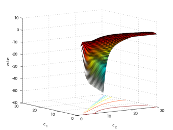
Case 1: $\beta=4$ and $\lambda=3$
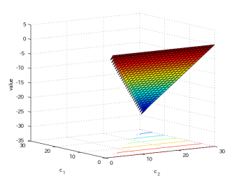
Case 2: $\beta=4$ and $\lambda=1$

Figure 1. For the case $\sigma=1$: (left) $\bar{v}_{c_{1},c_{2}}-c_{1}$ with respect to $c_{1}$ and $c_{2}$, (right) the value function $v_{c_{1}^{*},c_{2}^{*}}$ as a function of $x$.

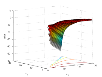
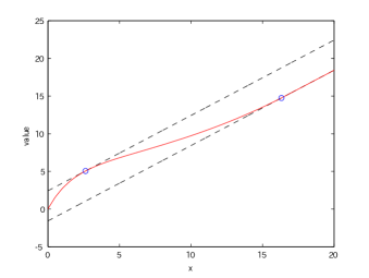
Case 1: $\beta=4$ and $\lambda=3$
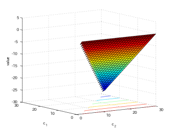
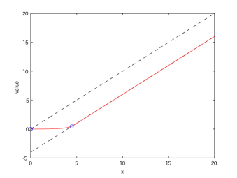
Case 2: $\beta=4$ and $\lambda=1$

Figure 2. For the case with $\sigma=0$: (left) $\bar{v}_{c_{1},c_{2}}-c_{1}$ with respect to $c_{1}$ and $c_{2}$, (right) the value function $v_{c_{1}^{*},c_{2}^{*}}$ as a function of $x$.

In our second experiment, we take $\beta\downarrow 0$ and see if the value function converges to the one under no-transaction costs as in [8]:

(6.2) $$\hat{v}_{a^{*}}(x):=\begin{cases}-\overline{R}^{(q)}(a^{*}-x),&\text{if $\mu>0$},\\ x,&\text{if $\mu\leq 0$},\end{cases}$$

for any $x\geq 0$, with the optimal barrier level

$$a^{*}:=\begin{cases}\left(\overline{Z}^{(q)}\right)^{-1}\left(\frac{\mu}{q}\right)>0&\text{if $\mu>0$},\\ 0&\text{if $\mu\leq 0$}.\end{cases}$$

We let $\lambda=3$ and consider the case $\mu>0$ (by choosing $\mathfrak{d}=2$) and also the case $\mu<0$ (by choosing $\mathfrak{d}=3$).

Figure 3 plots for each case the value function $v_{c_{1}^{*},c_{2}^{*}}(\cdot)$ for $\beta=10,5,1,0.5,0.1$ (dotted) together with the no-transaction case $\hat{v}_{a^{*}}(\cdot)$ (solid) as in (6.2). The circles on the plots indicate the points $(c_{1}^{*},v_{c_{1}^{*},c_{2}^{*}}(c_{1}^{*})),(c_{2}^{*},v_{c_{1}^{*},c_{2}^{*}}(c_{2}^{*}))$ and also $(a^{*},\hat{v}_{a^{*}}(a^{*}))$. It is easy to see that the value function is monotone in $\beta$ (uniformly in $x$), and converge to the no-transaction cost case as $\beta\downarrow 0$. The convergences of both $c_{1}^{*}$ and $c_{2}^{*}$ to $a^{*}$ are also observed. In fact, one can prove the convergence of value functions using the stability of viscosity solutions.

Proposition 6.1.

Let $v^{\beta}$ denote the value function corresponding to the dividend payment problem when the fixed transaction cost is $\beta$ (defined as above), and $\hat{v}$ the value function when there are no-transaction costs. Then $v^{\beta}$ converges to $\hat{v}$ uniformly as $\beta\downarrow 0$.

Proof.

From the definition of the problem, $v^{\beta}\leq\hat{v}$ and $v^{\beta}$ is decreasing in $\beta$ and hence it has a point-wise limit, which we will call $\tilde{v}$. The proof is completed if we can show that $\tilde{v}$ is a viscosity super-solution of the variational inequality that corresponds to the problem without transaction costs. But this is an immediate consequence of the stability result of the viscosity solutions (see e.g. Theorem 6.8 of [23] and Theorem 1 of [6]), since we can obtain the variational inequality in the no-transaction case by taking a limit in the case with transaction costs.

To get to uniform convergence from point-wise convergence we just proved, we appeal to Dini’s theorem to first show it on compacts. This indeed holds because we already know that $(v^{\beta})$ and $\hat{v}$ are continuous functions and $v^{\beta}\uparrow\hat{v}$ as $\beta\downarrow 0$. Now, because the slopes of $(v^{\beta})$ and $\hat{v}$ are all one above $c_{2}^{*}$ and $a^{*}$, respectively, and because $c_{2}^{*}$ can be shown to be bounded for any small $\beta$ (thanks to the convergence $c_{2}^{*}$ to $a^{*}$ as $\beta\downarrow 0$ or modifying the proof of Lemma 4.3), the uniform convergence holds. ∎

We also observe in the figures that for $\mu<0$, $c_{1}^{*}=0$. This can be shown analytically for any $\beta>0$.

Corollary 6.1.

If $\mu\leq 0$, we must have $c_{1}^{*}=0$.

Proof.

By the nature of the problem the value function $v_{c_{1}^{*},c_{2}^{*}}$ is dominated by that of the no-transaction cost case. By (6.2), we must have $v_{c_{1}^{*},c_{2}^{*}}(x)\leq x$ for any $x\geq 0$. Moreover, because $v_{c_{1}^{*},c_{2}^{*}}(0)=0$, $v_{c_{1}^{*},c_{2}^{*}}^{\prime}(0+)<1$ and hence, in view of the proof of Proposition 5.3, we must have $c_{1}^{*}=0$. ∎

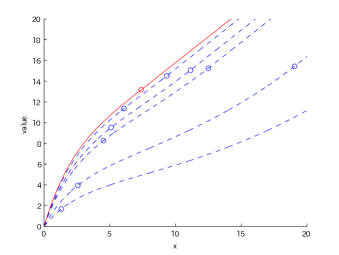
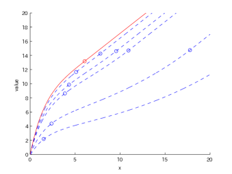
When $\mu>0$: (left) $\sigma=1$ and (right) $\sigma=0$
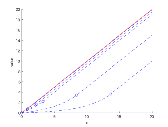
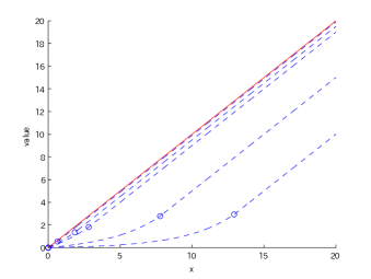
When $\mu<0$: (left) $\sigma=1$ and (right) $\sigma=0$

Figure 3. Convergence as $\beta\downarrow 0$.

References

- [1] S. Asmussen, F. Avram, and M. R. Pistorius. Russian and American put options under exponential phase-type Lévy models. Stochastic Process. Appl., 109(1):79–111, 2004.
- [2] B. Avanzi and H. U. Gerber. Optimal dividends in the dual model with diffusion. Astin Bull., 38(2):653–667, 2008.
- [3] B. Avanzi, H. U. Gerber, and E. S. W. Shiu. Optimal dividends in the dual model. Insurance Math. Econom., 41(1):111–123, 2007.
- [4] B. Avanzi, J. Shen, and B. Wong. Optimal dividends and capital injections in the dual model with diffusion. Astin Bull., 41(2):611–644, 2011.
- [5] F. Avram, Z. Palmowski, and M. R. Pistorius. On the optimal dividend problem for a spectrally negative Lévy process. Ann. Appl. Probab., 17(1):156–180, 2007.
- [6] G. Barles and C. Imbert. Second-order elliptic integro-differential equations: viscosity solutions’ theory revisited. Ann. Inst. H. Poincaré Anal. Non Linéaire, 25(3):567–585, 2008.
- [7] E. Bayraktar and M. Egami. Optimizing venture capital investments in a jump diffusion model. Math. Methods Oper. Res., 67(1):21–42, 2008.
- [8] E. Bayraktar, A. Kyprianou, and K. Yamazaki. On optimal dividends in the dual model. Astin Bull., 43(3), 2012.
- [9] L. Benkherouf and A. Bensoussan. Optimality of an policy with compound Poisson and diffusion demands: a quasi-variational inequalities approach. SIAM J. Control Optim., 48(2):756–762, 2009.
- [10] A. Bensoussan, R. H. Liu, and S. P. Sethi. Optimality of an policy with compound Poisson and diffusion demands: a quasi-variational inequalities approach. SIAM J. Control Optim., 44(5):1650–1676 (electronic), 2005.
- [11] J. Bertoin. Lévy processes, volume 121 of Cambridge Tracts in Mathematics. Cambridge University Press, Cambridge, 1996.
- [12] T. Chan, A. Kyprianou, and M. Savov. Smoothness of scale functions for spectrally negative Lévy processes. Probab. Theory Relat. Fields, 150:691–708, 2011.
- [13] R. A. Doney. Fluctuation theory for Lévy processes, volume 1897 of Lecture Notes in Mathematics. Springer, Berlin, 2007. Lectures from the 35th Summer School on Probability Theory held in Saint-Flour, July 6–23, 2005, Edited and with a foreword by Jean Picard.
- [14] M. Egami and K. Yamazaki. Phase-type fitting of scale functions for spectrally negative Lévy processes. arXiv:1005.0064, 2012.
- [15] J. Ivanovs and Z. Palmowski. Occupation densities in solving exit problems for Markov additive processes and their reflections. Stochastic Process. Appl., 122(9):3342–3360, 2012.
- [16] I. Karatzas and S. E. Shreve. Brownian motion and stochastic calculus, volume 113 of Graduate Texts in Mathematics. Springer-Verlag, New York, second edition, 1991.
- [17] A. E. Kyprianou. Introductory lectures on fluctuations of Lévy processes with applications. Universitext. Springer-Verlag, Berlin, 2006.
- [18] R. L. Loeffen. An optimal dividends problem with transaction costs for spectrally negative Lévy processes. Insurance Math. Econom., 45(1):41–48, 2009.
- [19] B. Øksendal and A. Sulem. Applied stochastic control of jump diffusions. Universitext. Springer, Berlin, second edition, 2007.
- [20] G. Peskir. A change-of-variable formula with local time on surfaces. In Séminaire de Probabilités XL, volume 1899 of Lecture Notes in Math., pages 69–96. Springer, Berlin, 2007.
- [21] P. E. Protter. Stochastic integration and differential equations, volume 21 of Stochastic Modelling and Applied Probability. Springer-Verlag, Berlin, 2005. Second edition. Version 2.1, Corrected third printing.
- [22] S. Thonhauser and H. Albrecher. Optimal dividend strategies for a compound poisson process under transaction costs and power utility. Stoch. Models, 27(1):120–140, 2011.
- [23] N. Touzi. Optimal stochastic control, stochastic target problems, and backward SDE, volume 29 of Fields Institute Monographs. Springer, New York, 2013. With Chapter 13 by Angès Tourin.
- [24] K. Yamazaki. Inventory control for spectrally positive Lévy demand processes. arXiv:1303.5163, 2013.
- [25] D. Yao, H. Yang, and R. Wang. Optimal dividend and capital injection problem in the dual model with proportional and fixed transaction costs. European Journal of Operations Research, 211:568–576, 2011.