An Experiment on Parallel Model Checking
of a CTL Fragment

Abstract

We propose a parallel algorithm for local, on the fly, model checking of a fragment of CTL that is well-suited for modern, multi-core architectures. This model-checking algorithm takes benefit from a parallel state space construction algorithm, which we described in a previous work, and shares the same basic set of principles: there are no assumptions on the models that can be analyzed; no restrictions on the way states are distributed; and no restrictions on the way work is shared among processors. We evaluate the performance of different versions of our algorithm and compare our results with those obtained using other parallel model checking tools. One of the most novel contributions of this work is to study a space-efficient variant for CTL model-checking that does not require to store the whole transition graph but that operates, instead, on a reverse spanning tree.

1 Introduction

Several model-checking methods address the state-explosion problem from a purely algorithmic perspective, for instance with the use of abstractions on the set of states (such as stubborn sets or symmetries) or symbolic techniques. Despite the fact that considerable progress has been made at the theoretical level, there are still classes of systems that cannot benefit from these advanced methods, like for example models that rely on real time constraints or on dynamic priorities. In this case, it is interesting to take benefit from the computation power—and increased amount of primary memory—provided by multi-processor and multi-core computers in order to handle very large state spaces.

In this paper, we propose a parallel algorithm for local, on the fly, model checking of a fragment of CTL that is well-suited for modern, multi-core architectures. We target shared-memory computers with a moderate number of cores (say 4 to 64) operating on a large shared memory space (typically from 16GB to 1TB of RAM). This description fits many available mid-range servers, but is also quite close to tomorrow’s mainstream desktop computers.

Our model-checking algorithm takes benefit from a parallel state space construction algorithm defined in a previous work [11] and share the same principles. First, we make no specific assumptions on the models that can be analyzed (we only assume that we know how to compute the successors of a given state and test them for equality). Second, we put no restrictions on the way states are distributed: in our solution, every process keeps a local share of the global state space and we do not rely on an a-priori static partition of the states. Finally, we put no restrictions on the way work is shared among processors; this means that our algorithm plays nicely with traditional work-sharing techniques, such as work-stealing or stack-slicing.

In this paper, we extend this state space construction algorithm by adding model checking capabilities. While the leading parallel model-checking tools are based on LTL model-checking, (see Sect. 5) we advocate the use of CTL. The choice of CTL derives from a number of desirable properties that we want for our parallel algorithm.

First, it must take advantage of parallelism and be compatible with our parallel state space generator. For this reason, the logic should preferably be branching time rather than linear time since model checking algorithms for linear time logics are strongly tied to depth-first-search (dfs) exploration techniques; and that dfs algorithms are “inherently sequential” (they belong to the class of P-complete problems [8, 3]). Parallel techniques for LTL model checking have been quite investigated however [1, 6] so we will compare our approach with these.

Secondly, we want an on-the-fly algorithm; only states essential for answering the model-checking problem should be enumerated. For this reason, model checking should be local rather than global; properties will be interpreted at the initial state rather than at all states.

Next, because the full state space may have to be enumerated (e.g. when checking a property that is true), we want it to be space-efficient. Hence, we shall accept that a small amount of information is recomputed every time it is needed rather than kept in storage.

For all these reasons, we decided to select a fragment of Computation Tree Logic (CTL) with state subformulas restricted to atomic propositions. This fragment strictly includes the logic used by popular tools like Uppaal. Though obviously less expressive than CTL, it implements a good trade-off between expressiveness and cost of verification when used to check large state spaces. While not yet implemented in our tool, it is possible to adapt our algorithm to model-check full CTL; more expressive logics will be considered in further work.

Contributions. We follow the classical approach of Clarke and Emerson [2] for CTL model-checking. During model-checking, we label each state of the system with the subformulas that are true at this given state. Labels are computed iteratively until we reach a fix-point, that is until we cannot add new labels. We consider two variants of this algorithm that differ by the amount of information on the transition relation that is stored. Both variants have two passes: a forward pass performs a constrained exploration of the state graph in which we start labeling each state with local information; a second, backward pass, propagates information towards the root of the state graph and checks if the resulting graph admits an infinite path.

In the first version of the algorithm, that we call RG (for reverse graph), we assume that, for every reachable state, we have a constant time access to the list of all its “parents”. In other words, we store the reverse transition relation of the state space. Algorithm RG is simply a parallel version of the algorithm in [2] that uses our parallel state space construction method. Our experimental results show that, even with this simple approach, we obtain a very good parallel implementation (that is with a good speedup) and a very good model-checking tool (that is with a good execution time when compared with other tools on a similar setup).

In the second version, we assume that we have direct access to only one of the parents, meaning that we may have to recompute some transitions dynamically. We call this second version RPG, for reverse parental graph. The advantage of the RPG version is to save memory space. Indeed, if we use the symbol $S$ to denote the number of reachable states, the RG algorithm as a space complexity in the order of $O(S^{2})$ in the worst-case, while it is of the order of $O(S)$ for the RPG version. We show, in our benchmarks, that the RPG version allows to compute bigger examples without sacrificing execution time.

Outline of the paper. In the next section, we summarize the parallel state space generation algorithm [11] that is used in our work. The model checking algorithms are defined in Sect. 3 using pseudo-code, while our parallel implementation is described in Sect. 4. Before concluding, we discuss the related work and compare our performances with the DiVinE[1] tool, a state of the art parallel model checker for LTL.

2 Parallel State Space Generation

State space generation is often a preliminary step for model checking behavioral formulas. This is a very basic operation: take a state that has not been explored; compute its successors and check if they have already been found before; iterate until there is no more new state to explore. Hence, a key point for performance is to use an efficient data structure for storing the set of generated states and for testing membership in this set. In [11], we propose an algorithm for parallel state space construction based on an original concurrent data structure, called a localization table (LT), that aims at improving spatial and temporal balance.

This approach is close in spirit to algorithms based on distributed hash tables, with the distinction that states are dynamically assigned to processors; i.e. we do not rely on an a-priori static partition of the state space. In our solution, every process keeps a share of the global state space in a local data structure. Data distribution and coordination between processes is made through the LT, that is a lockless, thread-safe data structure. The localization table is used to dynamically assign newly discovered states and can be queried to return the identity of the processor that owns a given state. With this approach, we are able to consolidate a network of local state repositories into an (abstract) distributed one without sacrificing memory affinity—data that are “logically connected” and physically close to each other—and without incurring performance costs associated to the use of locks to ensure data consistency.

The performance of our state space construction algorithm was evaluated on different benchmarks and compared with the results obtained using other solutions proposed in the literature. A first implementation of our algorithm showed promising results as we observed performances that are consistently better—both in terms of absolute speedup and memory footprint—than with other parallel algorithms. For example, this algorithm does consistently better than algorithms based on the use of static partitioning or than a similar approach based on the concurrent hash map implementation provided in the Intel Threading Building Blocks (TBB) library.

State space generation has a direct impact on the performance of the model-checking algorithm. For one thing, state space generation alone is enough to model-check reachability properties (of the form $A\Box(\phi)$). Moreover, for more complicated properties (see our benchmark results in Sect. 4), the time needed to explore the state space still makes up a big part of the model checking time.

3 Parallel Model Checking for a CTL Fragment

We build our model checking algorithm on top of the parallel state space generation algorithm of [11], described in the previous section. Our other design choices follow from our goal to target models with very large state spaces. More particularly, we choose to restrict ourselves to a fragment of CTL and to disallow the nesting of operators; that is, every subformula—denoted $\phi,\psi,\dots$—is a (boolean composition of) atomic propositions.

The logic used for model-checking essentially relies on three operators: Exist Until (EU), $E\,(\psi\cup\phi)$, that is true if there exists a trace (a path) in the state space such that $\psi$ has to hold until, at some position, $\phi$ holds; Always Until (AU), $A\,(\psi\cup\phi)$, that is true if the “until condition” holds on every trace; and finally the leadsto formula, $\psi\leadsto\phi$, that is true if, for every trace, whenever $\psi$ holds then necessarily $\phi$ will hold later. The last property can be expressed as $A\Box(\neg\,\psi\vee A\Diamond(\phi))$ in CTL. From the interpretation given in Table 1, we see that these operators define an expressive fragment of CTL (and also LTL).

Model-checking procedures for these operators will be described in Sections 3.2 to 3.4. In our implementation, we consider two variants—RG and RPG—of the algorithms. Both versions are based on two elementary phases: (1) a forward constrained exploration of the state graph using the state space construction discussed in Sect 2; followed by (2) a backward traversal and label propagation phase ensuring that the resulting graph is acyclic.

The backward traversal phase is only needed for AU and leadsto formulas, since checking EU formulas amounts to performing a constrained exploration of the state space (for instance, the formula $A\Box(\phi)$ is true if no state satisfies $\neg\phi$, which can be checked during the exploration phase). Consequently, our algorithm is not completely on-the-fly for these cases because the presence of a cycle is detected after the (constrained) state space is constructed, delaying the discovery of an invalid path. The last column of Table 1 indicates, for each formula, whether the backward phase is necessary.

Formulas	Interpretation in CTL	Forward	Backward
$E\leavevmode\nobreak\ (\psi\cup\phi)$	$E\leavevmode\nobreak\ (\psi\cup\phi)$	x
$A\leavevmode\nobreak\ (\psi\cup\phi)$	$A\leavevmode\nobreak\ (\psi\cup\phi)$	x	x
$E\Diamond(\phi)$	$E\leavevmode\nobreak\ (\mathrm{True}\cup\phi)$	x
$A\Diamond(\phi)$	$A\leavevmode\nobreak\ (\mathrm{True}\cup\phi)$	x	x
$E\Box(\phi)$	$\neg A\Diamond(\neg\phi)$	x	x
$A\Box(\phi)$	$\neg E\Diamond(\neg\phi)$	x
$\psi\rightsquigarrow\phi$	$A\Box(\neg\psi\vee A\Diamond\phi)$	x	x
$A\Box A\Diamond(\phi)$	${true}\rightsquigarrow\phi$	x	x

Figure 1: List of Supported Formulas.

3.1 Concepts and Notations

We assume that we perform model-checking on a Kripke System $\mathit{KS}(S,R,s_{0})$. We will use, interchangeably, the notation $\mathit{KS}$ for the Kripke structure $(S,R,s_{0})$ and $G$ for the directed graph $G(S,R)$, also called the state graph. In the RPG version of our algorithm, we make use of the Parental Graph of a Kripke System, that is a reverse spanning tree of the (currently computed) state graph.

Definition 1 (Parental Graph)

The directed graph, $PG(V_{p},E_{p})$, is a parental graph of $G(V,E)$ if: (1) $PG$ if a subgraph of $G$ that has the same vertices, that is $V_{p}=V$ and $E_{p}\subseteq E$, and (2) for every vertex $v\in V$, if $v$ is not the root of $G$ then $v$ has an in-degree of one in $PG$.

A simple way to obtain a parental graph, $PG$, when exploring the state graph, $G$, is to keep for every state, $s$, a vertex to the state in $G$ that was used to generate $s$ (and forget the others). The parental graph has nice properties. If $PG$ is a parental graph of $G$ and $G$ is acyclic then so is $PG$. Moreover, the set of leaves of $PG$ subsumes that of $G$; a leaf of $G$ is necessarily a leaf of $PG$.

In the remainder of the text, the expression $|S|$ is used to denote the cardinality of $S$ (the number of reachable states), while $|R|$ is the number of transitions. We assume that every state $s\in S$ is labeled with a value, denoted $\mathrm{suc}(s)$, that records the out-degree of $s$ in $\mathit{KS}$. The value of $\mathrm{suc}(s)$ is set during the forward exploration phase. Initially, $\mathrm{suc}(s)$ is the cardinality of the set of successors of $s$ in $\mathit{KS}$, that is $\mathrm{suc}(s)=\left|\{s^{\prime}\,|\,s\mathrel{R}s^{\prime}\}\right|$. We decrement this label during the backward traversal of the state graph; when the value of $\mathrm{suc}(s)$ reaches zero, we say that $s$ is cleared from the state graph. In our pseudo-code, we use the expression $\mathrm{suc}(s).\mathrm{dec}()$ to decrement the value of the label $\mathrm{suc}$ for the state $s$ in $\mathit{KS}$, and the expression $\mathrm{suc}(s).\mathrm{set}(i)$ to set the label of $s$ to some integer value $i$.

When we deal with the reverse parental graph version of our algorithm, we assume that we implicitly work with one particular parental graph of $\mathit{KS}$, denoted $\mathit{PKS}$. In this case, we assume that every state $s\in S$ is also labeled with a value, denoted $\mathrm{sons}(s)$, that records the out-degree of $s$ in $\mathit{KS}$. We also label each state $s\in S$ with a state, denoted $\mathrm{father}(s)$, that is the (unique) predecessor of $s$ in $\mathit{PKS}$. (The label $\mathrm{father}(s)$ makes sense only if $s$ is not the initial state, $s_{0}$, of $\mathit{KS}$.) Initially, the value of $\mathrm{sons}(s)$ is set to zero. The label will be incremented during the forward exploration, when we build $\mathit{PKS}$ (that is, we select the transitions from $\mathit{KS}$ that will be stored in $\mathit{PKS}$). This operation is denoted $\mathrm{sons}(s).\mathrm{inc}()$ in our pseudo-code. We will decrement the value of $\mathrm{sons}(s)$ during the backward traversal phase.

3.2 Checking EU properties

Checking EU properties for the initial state is standard, except that we perform the forward phase concurrently, on all states. this can be done on the fly in a single, forward pass. To check the formula $E\,(\psi\cup\phi)$, we explore the state space until a state is found such that either (1) $\phi$ holds and no more state has to be explored, or (2) $\neg\psi\wedge\neg\phi$ holds. In the first case, the algorithm reports success; all states obeying $\phi$ terminate a (possibly empty) path of states rooted at the initial state and all obeying $\psi$. In the second case, we have found a counter-example; a state obeying neither $\psi$ nor $\phi$, meaning that the property is false at the initial state. The check function is the same for the two versions of our algorithm, whether based on the reverse graph or the reverse parental graph data structure.

⬇

1function BOOL check_a($\psi$ : pred, $\phi$ : pred, $s_{0}$ : state)

2 Stack A $\leftarrow$ new Stack($\emptyset$) ;

3 //Start with the forward exploration

4 if forward_check_a($\psi$ , $\phi$, $s_{0}$, A) then //If all forward constraints are respected

5 return backward_check_a($s_{0}$, A) //start the backward phase

6 else return FALSE // We found a problem during the forward exploration

Listing 1: Algorithm for the formula $A\,(\psi\cup\phi)$—function check_a

3.3 Checking AU Properties

For checking the formula $A\,(\psi\cup\phi)$, as for EU properties, we stop exploring a path when we find a state such that (1) $\phi$ holds or (2) $\neg\psi\wedge\neg\phi$ holds. If an occurrence of case (2) is found, we have a counter-example to the property false. Otherwise, we start backward traversal phase in order to detect cycles. Indeed, the property $A\,(\psi\cup\phi)$ is false if there is an infinite path of states (starting from $s_{0}$) that all obey $\psi$. We call this second phase the clearing phase, because it consists in recursively removing leaf nodes from the graph. This process ends either when the only remaining state is the initial state (meaning that the property is true), or when no states with out-degree zero can be found (in which case we know that there is a cycle). The validity of this method follows from the fact that a finite Directed Acyclic Graph (DAG) has at least one leaf.

We give the pseudo-code for checking $A\,(\psi\cup\phi)$ in Listing 1. The inputs are the atomic properties $\psi$ and $\phi$ and the initial state $s_{0}$. The algorithm makes use of a stack A to collect the states at which $\phi$ holds during the forward exploration phase. The procedure uses two auxiliary functions, forward_check_a and backward_check_a, that depends on the version of the algorithm. We start by defining these helper functions for the Reverse Graph version.

Algorithm for the Reverse Graph version (RG). We give the pseudo-code for the function forward_check_a (for the RG version) in Listing 2. The last parameter of this function, A, is a stack that is used to collect the leaf nodes of the state graph, that is the states where $\phi$ holds. These states are the starting points in our backward traversal of the graph.

During the forward exploration phase (function forward_check_a) each state $s$ is labelled with its number of successors in the initial state graph (the Kripke structure). During the backward traversal phase (function backward_check_a), this label is decremented each time a successor of $s$ is removed; decrementations are done in parallel. Intuitively, a state can be removed as soon as it is cleared. We never actually remove a state from the graph. Instead, when a processor changes the label of a state $s$ to $0$, we also decrement the labels of all the parents of $s$ in the graph. Hence the choice of storing the reverse of the transition function in the data structure.

In the function backward_check_a, see Listing 2, we start by clearing all the states in A which are, by construction, the states $s$ such that $\mathrm{suc}(s)$ is nil. When a state is cleared, we decrement the labels of all its parents ($suc(s^{\prime}).dec()$) and check which ones can be cleared ($suc(s^{\prime})==0$). The algorithm stops if the initial state, $s_{0}$, can be cleared or if there are no more states to update.

⬇

1function BOOL forward_check_a($\psi$ : pred, $\phi$ : pred, $s_{0}$ : state, A : Stack)

2 Set S $\leftarrow$ new Set($s_{0}$) ; Stack W $\leftarrow$ new Stack($s_{0}$) ;

3 while (W is not empty) do

4 s $\leftarrow$ W.pop();

5 if (s $\vDash\phi$) then

6 suc(s).set(0) ; //We clear state s from KS

7 A.push(s)

8 elsif (s $\vDash\psi$) then //We tag s with its number of successors

9 suc(s).set(number of successors of s in KS) ;

10 if (suc(s) = 0) //Check if s is not a dead state

11 return FALSE

12 forall s’ successor of s in KS do //and continue the exploration

13 if (s’ $\notin$ S) then

14 S $\leftarrow$ S $\cup$ {s’} ; //s’ is a new state

15 W.push(s’)

16 else return FALSE

17 return TRUE

18

19function BOOL backward_check_a($s_{0}$ : state, A : Stack)

20 while (A is not empty) do

21 s $\leftarrow$ A.pop() ;

22 if (s = $s_{0}$) then //The property is true if

23 return TRUE //we reach the initial state

24 forall s’ parent of s in KS do //Otherwise we check if the

25 suc(s’).dec() ; //predecessors of s can be cleared

26 if (suc(s’) = 0) then A.push(s’)

27 return FALSE

Listing 2: Forward and backward exploration for $A\,(\psi\cup\phi)$ with Reverse Graph

Algorithm for the Reverse Parental Graph version (RPG). The function for the RPG version is only slightly more complicated, because we need to recompute some successors in the transition relation: we can only access one of the parents of a state in constant time (which we call the father of the state). The pseudo-code for the forward exploration phase (function forward_check_a) is essentially the same as in Listing 2; this is why it is omitted here. Compared to the RG version, we only need to add two additional statements when adding a new state (around line 15 in Listing 2): assuming that the state $s$ is generated from a state $s^{\prime}$, we set the value of the father for the newly generated state ($father(s).set(s^{\prime})$) and increment the number of sons of the father $sons(s).inc()$). This information is used during the backward traversal to track non cleared leaves.

We give the pseudo-code for the backward traversal phase in Listing 3. During this phase, we follow the parental graph structure to “propagate” the cleared states toward the root of the state graph. The algorithm alternates between two behaviors, clearing and collecting. The clearing behavior is similar to the pseudo-code for the RG algorithm, with the difference that we decrement only the father of a state and not all the predecessors. When there are no more labels to decrement—and if the root state is not yet cleared—the algorithm starts looking for states that can be cleared. For this, we test all the states $s$ such that $sons(s)==0$; that is, such that all the sons of $s$ have been cleared (in the parental graph). In this case, to check if $s$ can be cleared, we have to recompute all its successors in $\mathit{KS}$ and check whether they have also been cleared (if their $\mathrm{suc}$ label is zero).

⬇

1function BOOL backward_check_a($s_{0}$ : state, A : Stack)

2 over $\leftarrow$ FALSE

3 while (not over)

4 while (A is not empty) do

5 //Clearing

6 s $\leftarrow$ A.pop() ;

7 if (s = $s_{0}$) then //The property is true if

8 return TRUE //we reach the initial state

9 s’ $\leftarrow$ father(s) ; //Otherwise we check if

10 sons(s’).dec() ; //the father of s can be cleared

11 suc(s’).dec() ;

12 if (suc(s’) = 0) then A.push(s’)

13 //Collecting: if we have no more states to clear in A we try to find

14 //candidates among the states with no children in $\mathit{PKS}$

15 forall s such that sons(s) $=$ 0 and suc(s) $\neq$ 0 in KS do

16 if test(s) then

17 suc(s).set(0) ;

18 A.push(s)

19 if (A is empty) then

20 over $\leftarrow$ TRUE //No good candidate was found, end backward search

21 return FALSE

22

23function BOOL test(s : state)

24 forall s’ successor of s in KS do

25 if suc(s’) $\neq$ 0 then

26 return FALSE //at least one successor is not cleared

27 return TRUE

Listing 3: Backward exploration for $A\,(\psi\cup\phi)$ with Reverse Parental Graph

The advantage of this strategy is that we do not have to consider all the states in the graph but just a subset of them. Indeed, we know that if $\mathit{KS}$ is a acyclic (is a DAG) then $PG$ has at least one leaf that is also a leaf in $G$ [9]. Hence, this subset is enough to test the presence of a cycle. Conversely, the drawback of this approach is that we may try to clear the same vertex several times, which may be time consuming.

3.4 Checking Leadsto Properties

To check the formula $\psi\rightsquigarrow\phi$, we need to prove that no cycle can be reached from a state where $\psi$ holds, without first reaching a state where $\phi$ holds. Indeed, otherwise, we can find an infinite path where

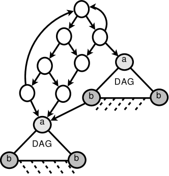
Figure 2: Formula $a\rightsquigarrow b$.

$\phi$ never holds after an occurrence of $\psi$. Figure 2 shows an example of graph for which the formula is valid.

This observation underlines the link between checking the formula $\psi\rightsquigarrow\phi$ locally—for the initial state—and checking the validity of $A\Diamond(\phi)$ globally—at every state where $\psi$ holds. As a consequence, we can use an approach similar to the one used for AU properties in the previous section. The main difference is that, instead of clearing the initial state, we have to clear all the states where $\psi$ holds. Hence, the pseudo-code for the leadsto formulas is similar to that of AU formulas (this is why it is omitted here), the main difference is in the termination condition: the function returns true if all the states where $\psi$ holds are cleared.

3.5 Correctness and Complexity of our Algorithms

Proofs of correctness (termination, completeness and soundness) and a precise study of the complexity of our algorithms can be found in [9]. We just discuss here the worst-case complexity in the sequential case, and for formulas $A\,(\psi\cup\phi)$. The results for this case can be generalized to our whole logic. (Inside asymptotic notations, we use the symbols $S$ and $R$ when we really mean $|S|$ and $|R|$.)

The algorithm given in Sect. 3.3 may inspect every state in the Kripke Structure $\mathit{KS}$ and, for every transition, it may update one label. Therefore, its worst-case time complexity is in the order of $O(S+R)$ for the RG algorithm. The complexity is higher in the RPG version since, for each altered state, we may have to recompute the successors for all the reachable states $s$ such that $\mathrm{sons}(s)$ is nil. Hence, solving a simple recurrence, we can prove that the time complexity is in the order of $O(S\cdot(R-S))$ for the RPG version. Since the number of transitions in $\mathit{KS}$ is bounded by $|S|^{2}$, we obtain a complexity in the order of $O(S^{2})$ for the RG version and of $O(S^{3})$ for the RPG variant. Concerning the space complexity, the RPG version is in the order of $O(S)$, while the RG version is linear in the size of the graph, that is in the order of $O(S+R)$ (or $O(S^{2})$).

We show in our experiments that the decision to favor “space-efficiency” (in the case of the RPG version) is quite interesting. In particular, on some examples, the RPG version may run faster than the RG version because it needs to “write less information” in main memory, an effect that is not visible if we only look at the theoretical complexity. More importantly, memory is one of the key resources used during model-checking. Indeed, it is common to exhaust the available memory during verification.

4 Implementation and Experimental Results

In the code presented in Sect. 3, no underlying computational model was make precise. The code can be easily adapted to a Parallel RAM model, following a Single Program Multiple Data (SPMD) programming style. In this section, we discuss the details surrounding the parallel implementation of our algorithms, then report on a set of experiments performed to evaluate their effectiveness.

4.1 Parallel Implementation of our Algorithm

In a SPMD context, all processing units will execute the same functions (the one defined in Listings 1–3). Following this approach, the (forward) exploration phase and the (backward) cycle detection phase can both be easily parallelized. Then, for the model-checking function themselves—for instance the function check_a—we only need to synchronize the termination of the forward exploration with the start of the backward label propagation. At each point, a processing unit can terminate the model-checking process if it can prove (or disprove) the validity of the formula before the end of the exploration phase. Actually, most of the burden of parallelizing our algorithm is hidden inside the use of our specialized, lock-free data structures.

We consider a shared memory architecture where all processing units share the state space (using the mixed approach presented in [11]) and where the working stacks are partially distributed (such as the stacks W and A used in our pseudo-code). For most of our pseudo-code, it is enough to rely on atomic “compare and swap” primitives to protect from parallel data races and other synchronization issues; typically, compare-and-swap primitives will be used when we need to test the value of a label or when we need to update the label of a state (for instance with expressions like $\mathrm{sons}(s).\mathrm{dec}()$). Together with the compare-and-swap primitive, we use our combination of distributed, local hash tables with a concurrent localization table to store and manage the state space.

For the RG version of the algorithm, we can ensure the consistency of our algorithm by protecting all the operations that manipulate a state label. (We made sure, in our pseudo-code, that every operation only affects one state at a time.) The parallel version of RPG is a bit more involved. This problem is related to the behavior of the collecting operations of the backward exploration (see the comment on line 14 of Listing 3)—and in particular the function test—that needs to check all the successors of a state to see if they are cleared. First, this code is not atomic and it is not practical to put it inside a critical section (it would require a mutex for every state). If two processors collect the same state, then the father of this state could be decremented twice, during the clearing operations. Second, collecting must be performed after all processors have finished the clearing operations, otherwise the algorithm may end prematurely (see [9] for a complete explanation.) We solve the concurrency issues for the RPG version through the synchronization of all processors before both clearing and collecting. Then, we take advantage of our distributed local state repositories to avoid problems due to concurrent access; each processor can perform the collecting operations only over the states that it owns. Finally, we use a work-stealing strategy (see [11]) to balance the work-load between the different phases of our algorithm; for instance, whenever a thread has no more state to clear, it tries to “steal” non-cleared states from other processors.

4.2 Experimental Results

We have implemented the parallel versions of our model-checking algorithm and evaluated their performances on several benchmarks. Experimental results presented in this section were obtained on a Sun Fire x4600 M2 Server configured with 8 dual core opteron processors and 208 GB of RAM memory, running the Solaris 10 operating system. (The complete set of experiments can be found in [9].) We give results obtained on 8 classical models—a Token Ring protocol; the Peg-Solitaire board-game; …—with a mix of valid and invalid properties. We experimented with all the formulas: reachability ($E\Diamond\phi$), safety ($A\Box\phi$ and $E\Box\phi$), liveness ($A\Diamond\phi$) and leadsto ($\psi\rightsquigarrow\phi$).

Speedup Analysis: we study the relative speedup and the execution time for our algorithms. In addition, we also give the separate speedup obtained in each phase of the algorithm—during the exploration (forward) and cycle detection (backward) phases—in order to better analyze the advantages of our approach.

Figure 4 shows speedup analysis for the RPG version of our algorithm. We only show the results for two models—a Token Ring with 22 bases (TK22) and a Solitaire game with 33 pegs—since they are representative of the results obtained with our complete benchmark. These models have different execution profiles which impacts significantly the overall performance. The main difference is the time spent in the backward traversal phase. Figure 4 shows a series of bar charts putting in evidence the time required for each phase of the algorithm (exploration and cycle detection). In addition, we compare our approach (RG and RPG) with a third algorithm (NO_GRAPH) that uses the same code as RG but recomputes predecessor states instead of storing them (this is possible only because, for this particular benchmark, we know how to compute the predecessors of a state). We have observed two main categories of behaviors in this analysis.

negligible backward traversal: the time spent in the backward exploration phase is negligible compared to the overall execution time (e.g. model TK22 in Fig. 4, 4). This is the case, for instance, if the property is false and the cycle detection phase terminates early. In this category of experiments, there are no significant differences between RG and RPG, mainly because the gain in performance during the forward exploration phase outweighs the extra work performed during the cycle detection phase;

complete backward traversal: the cycle detection phase needs to run through all the state space (e.g. model SOLITAIRE in Fig. 4, 4). We observe a significant difference in performance between the RG and RPG versions in this case. The extra work performed by the RPG version becomes the dominant factor.

a) Speedup b) Execution Time Figure 3: Speedup and execution time analysis for Token Ring and Solitaire models.

Figure 4: Comparison with a Standard Algorithm.

These experiments confirm that RPG is a good choice when we are limited by the memory space: although it may require more computations (in our examples, we may loose a factor of $5$ in execution time), it can be applied on models that are not tractable with the RG version because of the space needed to store the transitions. For instance, for the Peg Solitaire model with 37 pegs (that has $3.10^{9}$ states and $3.10^{10}$ transitions), the RPG only needs 15 GB of memory while, with the RG version, we would need 240 GB of memory just to store the transitions.

5 Related work and Comparisons With Other Tools

Several works address the problem of designing efficient, parallel model-checking algorithms. Most of the proposals follow an “automata-theoretic approach” for LTL model checking. In this context, the difficulty is to adapt the cycle detection algorithms (Tarjan or Nested-DFS), which are inherently sequential. Two works stand out: one with a mature implementation, DiVinE [1], with the owcty + map algorithm; another with a prototype, named LTSmin, with the mc-ndfs algorithm [6]. They mostly differ by the algorithm used to detect cycles.

DiVinE combines two algorithms, owcty and map, that result in “a parallel on-the-fly linear algorithm for model checking weak LTL properties” (weak LTL properties are those expressible by an automata that has no cycle with both accepting and no-accepting states on its path). If the LTL property does not meet this requirement, the algorithm complexity may be quadratic. The multi-core nested DFS (mc-ndfs) algorithm [6] is a recent extension of the swarm [4] distributed algorithm to a multi-core setting. The authors in [6] propose a multi-core version with the distinction that the storage state space is shared among all workers in conjunction with some synchronization mechanisms for the nested search. Even if, in the worst-case, all the processors may duplicate the same work, this approach has a linear complexity (given a fixed number of processors).

In contrast with the number of solutions proposed for parallel LTL model checking, just two specifically target CTL model checking on shared memory machines: Inggs and Barringer work [5] supports CTL^∗, while van de Pol and Weber work [7] supports the $\mu$-calculus.

Comparison with DiVinE. We now compare our algorithms with DiVinE [1], which is the state of the art tool for parallel model checking of LTL. The results given here have been obtained with DiVinE 2.5.2, considering only the best results given by the owcty or map, separately. This benchmark (experimental data and examples are available in report [10]) is based on the set of models borrowed from DiVinE on which, for a broader comparison, we check both valid and non valid properties. Figure 7 shows the exact set of models and formulas that are used. All experiments were carried out using 16 cores and with an initial hash table sized enough to store all states. The DiVinE experiments were executed with flag (-n) to remove counter-example generation.

Model Formula Results Anderson (AN) $18\cdotp 10^{6}$ states F1:(-cs_0) ==> (cs_0) false F2:A[]<>(cs_0 or ... or cs_n) true Lamport (LA) $38\cdotp 10^{6}$ states. F1:(wait_0 and (- cs_0)) ==> (cs_0) false F2:(- cs_0) ==> (cs_0) false F3:A[]<>(cs_0 or ... or cs_n) true Rether (RE) $4\cdotp 10^{6}$ states F1:A[]<>(nrt_0) true F2:A[]<>(rt_0) false Szymanski (SZY) $2\cdotp 10^{6}$ states . F1:(wait_0 and (- cs_0)) ==> (cs_0) false F2:(- cs_0) ==> (cs_0) false F3:A[]<>(cs_0 or ... or cs_0) true Figure 5: Formulas and Models for our Comparison.

M  Formula owcty map reverse parental T.(s) M.(Gb) T.(s) M.(Gb) T.(s) M.(Gb) T.(s) M.(Gb) AN F1: false 61.3 3.3 110.2 5.5 28.8 2.8 94.4 1.8 F2: true 79.5 7.4 110.5 4.8 26.4 2.9 50.4 1.8 LA F1: false 1.6 1.1 1.4 1.1 42.4 5.1 74.2 3.3 F2: false 1.4 1.1 1.7 1.2 47.6 5.6 327.2 3.6 F3: true 153.6 14.1 282.8 12.1 51.0 5.6 370.4 3.7 RE F1: true 12.0 1.8 20.1 1.3 5.0 0.7 12.0 0.6 F2: false 13.2 1.8 1.2 0.3 3.4 0.7 7.8 0.6 SZY F1: false 8.5 0.9 7.0 0.5 2.2 0.3 1.4 0.2 F2: false 9.8 0.9 6.6 .5 4.2 0.3 39.6 0.3 F3: true 9.0 0.9 24.7 0.6 3.8 0.3 32.8 0.3 Figure 6: Table of results.

Figure 7: Comparison with divine (reverse = RG, parental = RPG).

Figure 7 shows for each model the execution time (T.) in seconds and the memory peak (M.) (in GB). Figure 7 summarizes these results using the normalized weighted sum of the memory footprint and the execution time, separated for valid and non valid formulas.

Algorithms owcty and map show better overall results when the formula is not valid (FALSE). By contrast, reverse holds the best execution time when the formula is valid. Regarding the RPG version of our algorithm, our results show that it holds the best memory footprint among all results, it uses on average $2$ to $4$ times less memory than map and owcty when the formula is valid. In addition, regardless of its “cubic” worst-case complexity, it shows good results when compared to map and owcty. For instance, it is able to verify a valid formula on average using $4$ times less memory than owcty with a limited slow-down ($\approx 1.8$ times slower).

To conclude, for the set of models and formulas used in this benchmark, both RPG and RG delivered good results when compared to DiVinE. For instance, RG has a better performance in both time and memory usage when compared with DiVinE (map and owtcy). Finally, RPG proved to be the most space conscious algorithm—the one to choose for the biggest models—without sacrificing too much the execution time.

6 Conclusion

We have described ongoing works concerning parallel (enumerative) model-checking algorithms for finite state systems. We define two versions of a new model checking algorithm that support an expressive fragment of both CTL and LTL. These algorithms are based on the standard, semantic model-checking algorithm for CTL but specifically target parallel, shared memory machines. Our two versions differ by the amount of information they need to store: a Reverse Graph (RG) version that explicitly stores the complete transition relation in memory, and a Reverse Parental Graph (RPG) that relies on a spanning tree.

We use the reverse parental graph structure as a mean to fight the state explosion problem. In this respect, this approach has a similar impact—on the space—than algorithmic techniques like sleep sets (used with partial-order methods), but with the difference that we do not take into account the structure of the model. Moreover, our approach is effective regardless of the formalism used to model the system. For instance, it is particularly useful in cases where it is not possible to compute the “inverse” of the transition relation.

Our prototype implementation shows promising results for both the RG and RPG versions of the algorithm. The choice of a “labeling algorithm” based on the out-degree number has proved to be a good match for shared memory machines and a work stealing strategy; we consistently obtained speedups close to linear with an average efficiency of $75\%$. Our experimental results also showed that the RPG version is able to outperform the RG version for some categories of models.

Using our work, one can easily obtain a parallel algorithm for checking any CTL formula $\Phi$ by running one instance of our algorithms (for the AU and EU formulas) for each subformula of $\Phi$. But this approach, as such, is too naive. For future works, we are considering improvements of our algorithms that support full CTL formulas without having to manage several copies of our labels ($\mathrm{sons}$ and $\mathrm{suc}$) in parallel, which could have an adverse effect on memory consumption.

References

- [1] J. Barnat, L. Brim, M. Češka, and P. Ročkai. DiVinE: Parallel Distributed Model Checker. In Parallel and Distributed Methods in Verification and High Performance Computational Systems Biology (HiBi/PDMC 2010), pages 4–7. IEEE, 2010.
- [2] Edmund M. Clarke and Allen Emerson. Design and synthesis of synchronization skeletons using branching time temporal logic. In Logics of Programs, volume 131 of LNCS, pages 52–71. 1982.
- [3] Raymond Greenlaw, H. James Hoover, and Walter L. Ruzzo. Limits to Parallel Computation: P-Completeness Theory. Oxford University Press, USA, 1995.
- [4] G. J Holzmann, R. Joshi, and A. Groce. Swarm verification. In Proc. of the 23rd IEEE/ACM Int. Conference on Automated Software Engineering, pages 1––6, 2008.
- [5] Cornelia P. Inggs and Howard Barringer. CTL* model checking on a shared-memory architecture. Formal Methods in System Design, 29(2):135–155, July 2006.
- [6] A. W. Laarman, R. Langerak, J. C. van de Pol, M. Weber, and A. Wijs. Multi-Core nested Depth-First search. In Proc. of the 9th International Symposium on Automated Technology for Verification and Analysis, ATVA 2011, LNCS, 2011.
- [7] Jaco van de Pol and Michael Weber. A Multi-Core solver for parity games. In Proc. of the 7th International Workshop on Parallel and Distributed Methods in verifiCation (PDMC 2008), volume 220(2) of ENTCS, pages 19–34, 2008.
- [8] John H. Reif. Depth-first search is inherently sequential. Information Processing Letters, 20(5):229–234, 1985.
- [9] Rodrigo T. Saad. Parallel Model Checking for Multiprocessor Architecture. PhD thesis, Institut National des Sciences Appliquées, Toulouse, France, December 2011.
- [10] Rodrigo T. Saad, Silvano Dal Zilio, and Bernard Berthomieu. Parallel Model Checking with Lazy Cycle Detection—MCLCD. Technical Report 12139, LAAS-CNRS, 2012 (http://hal.archives-ouvertes.fr/hal-00669752/en).
- [11] Rodrigo T. Saad, Silvano Dal Zilio, and Bernard Berthomieu. Mixed Shared-Distributed hash tables approaches for parallel state space construction. In Int. Symposium on Parallel and Distributed Computing (ISPDC 2011), July 2011.