Constraints on anomalous $tcZ$ coupling from $\bar{B}\to\bar{K}^{*}\mu^{+}\mu^{-}$ and $B_{s}\to\mu^{+}\mu^{-}$ decays

Abstract

In this paper, we analyze the possible anomalous $tcZ$ coupling effects in the $b\to s$ mediated decays $\bar{B}\to\bar{K}^{*}\mu^{+}\mu^{-}$ and $B_{s}\to\mu^{+}\mu^{-}$. After exploiting the available experimental data, the combined constraints on the anomalous coupling $X_{ct}^{L}$ are derived. It is found that, the bound on the magnitude $|X_{ct}^{L}|$ is dominated by the branching ratios of these two decays. Furthermore, one sign-flipped solution is excluded by the longitudinal fraction of $\bar{B}\to\bar{K}^{*}\mu^{+}\mu^{-}$ at the low dilepton mass region. After considering the combined constraints, for general complex coupling $X_{ct}^{L}$, the predicted upper bound on $\mathcal{B}(t\to cZ)$ are compatible with that from the recent CMS direct search. In particular, for the case of real coupling $X_{ct}^{L}$, the upper bound reads $\mathcal{B}(t\to cZ)<6.3\times 10^{-5}$, which is much lower than the current CMS bound but still accessible at the LHC. With improved measurements at the LHC, the colser correlations between the $t\to cZ$ and $b\to s$ mediated (semi-) leptonic decays are expected in the near future.

1 Introduction

In the Standard Model (SM), the flavor-changing neutral current (FCNC) transitions are forbidden at tree level and highly suppressed at one-loop level due to the Glashow-Iliopoulos-Maiani (GIM) mechanism [1]. Such processes may receive competing contributions from possible new physics (NP) beyond the SM, as a result of which the expected rates related to these processes can be significantly altered. Thus the FCNC processes are promising probes of the SM and its extensions.

For the top quark in particular, the FCNC decays $t\to qZ$ (where $q$ denotes a $c$- or $u$-flavored quark) are predicted to be far below the detectable level within the SM, with branching ratios of order of $10^{-10}$ [2, 3]. However, there are various NP models that may enhance these processes significantly [4, 5]. This makes any positive signal of these decays an indirect evidence of NP beyond the SM. Search for the top quark FCNC decays has been performed at the Tevatron [6, 7] and the LHC [8, 9]. The best upper limits on branching ratio of $\mathcal{B}(t\to qZ)<0.24\%$ at $95\%$ C.L. are recently established by the CMS collaboration [9]. Improved direct searches will be available at the LHC due to its large top sample in prospect. The discovery potential of $\mathcal{B}(t\to qZ)$ is of the order $10^{-4}$ at the ATLAS [10, 11] and the CMS [12].

However, when studying the phenomena of the $t\to qZ$ transition, or equivalently an effective anomalous $tqZ$ coupling, at high-energy colliders, the low-energy processes involving the top quark loops should also be taken into account [13, 14, 15, 16, 17, 18, 19, 20, 21]. In our previous works [22, 23, 24], we have investigated the top quark anomalous coupling effects in rare B and K-meson decays. For the anomalous $tcZ$ coupling in particular, it is found that the dominant constraints come from the $B_{s}\to\mu^{+}\mu^{-}$ decay. As another $b\to s\mu^{+}\mu^{-}$ process, the $\bar{B}\to\bar{K}^{*}\mu^{+}\mu^{-}$ decay has been investigated in the literature [25, 26, 27, 28, 29, 30] and shown to be able to provide complementary information about the potential NP contributions [31, 32, 33, 34, 35]. Its subsequent $K^{*}\to K\pi$ processes allow to offer a large number of observables in the fully differential distribution through an angular analysis of the $K\pi\mu^{+}\mu^{-}$ final state [36, 37]. Furthermore, the hadronic uncertainties in some angular observables cancel each other, which makes theoretical predictions precise [38, 39]. On the experimental side, the $\bar{B}\to\bar{K}^{*}\mu^{+}\mu^{-}$ decays have been measured by the experiments BaBar [40], Belle [41], CDF [42, 43] and LHCb (with an integrated luminosity of $0.37\,{\rm fb}^{-1}$) [44]. In the near future the LHCb collaboration expects to improve these measurements by using an integrated luminosity of $1.5\,{\rm fb}^{-1}$ data [45].

Recently, the first evidence for the decay $B_{s}\to\mu^{+}\mu^{-}$ has been announced by the LHCb collaboration [46]. The observed rate $\mathcal{B}(B_{s}\to\mu^{+}\mu^{-})=(3.2_{-1.2}^{+1.5})\times 10^{-9}$ is in good agreement with the SM prediction. In this paper, motivated by the LHCb result, we shall update the bound on the anomalous $tcZ$ coupling obtained in our previous work [24] with this recent data. After performing a model-independent study of the anomalous $tcZ$ coupling effects in the $\bar{B}\to\bar{K}^{*}\mu^{+}\mu^{-}$ decays, we derive the combined bounds on its strength by these two decay modes. The implications for the direct search of the rare $t\to cZ$ decays at the LHC are also discussed.

Our paper is organized as follows: In section 2, we introduce the effective Lagrangian describing the anomalous $tqZ$ interactions. Section 3 gives a short review on the $B_{s}\to\mu^{+}\mu^{-}$ and $\bar{B}\to\bar{K}^{*}\mu^{+}\mu^{-}$ decays and also the anomalous $tcZ$ coupling effects in these two decays. In section 4, we give our detailed numerical results and discussions. We conclude in section 5. The relevant formulae for our analysis are shown in the Appendices.

2 Effective Lagrangian for anomalous $tqZ$ couplings

From the viewpoint of effective field theory, the SM can be considered as an effective low-energy theory of an underlying theory at a scale $\Lambda$ which is much higher than the electroweak scale $v=246\,{\rm GeV}$ [47]. The NP effects above the electroweak scale can be encoded in the higher dimensional interaction terms involving only the SM fields and invariant under the SM gauge symmetry. In particular, the FCNC transitions $t\to qZ$ can be described by a few dimension 6 operators [48, 49]. These operators can contribute to the $tqZ$ vertices, resulting an equivalent description by the effective Lagrangian [48, 50, 51]

$$\mathcal{L}_{tqZ}= +\frac{g}{2\cos\theta_{W}}\bar{q}\gamma^{\mu}(X_{qt}^{L}P_{L}+X_{qt}^{R}P_{R})tZ_{\mu}$$

$$+\frac{g}{2\cos\theta_{W}}\bar{q}\frac{i\sigma^{\mu\nu}p_{\nu}}{m_{Z}}(\kappa_{qt}^{L}P_{L}+\kappa_{qt}^{R}P_{R})tZ_{\mu}+{\rm h.c.},$$ (2.1)

with $P_{L,R}=(1\mp\gamma^{5})/2$. The dimensionless couplings $X_{qt}^{L,R}$ and $\kappa_{qt}^{L,R}$ are complex generally and can be written in terms of its magnitude and phase as, for example, $X_{ct}^{L}\equiv\lvert X_{ct}^{L}\rvert e^{i\theta_{ct}^{L}}$. This Lagrangian has been employed in phenomenological analyses related to top-quark physics [4, 5].

3 Theoretical Framework

In this section, we shall first introduce the theoretical framework of the $B_{s}\to\mu^{+}\mu^{-}$ and $\bar{B}\to\bar{K}^{*}l^{+}l^{-}$ decays, and then discuss the anomalous $tqZ$ coupling effects in these two decays.

3.1 Effective Hamiltonian

In the SM, the effective Hamiltonian for the $b\to sl^{+}l^{-}$ transitions read [52, 53]

$$\mathcal{H}_{\rm eff}=-\frac{4G_{F}}{\sqrt{2}}\left(\lambda_{t}\mathcal{H}_{\rm eff}^{(t)}+\lambda_{u}\mathcal{H}_{\rm eff}^{(u)}\right),$$ (3.1)

with the products of the CKM matrix elements $\lambda_{q}\equiv V_{qb}V_{qs}^{*}$ and

$$\mathcal{H}_{\rm eff}^{(t)}=C_{1}\mathcal{O}_{1}^{c}+C_{2}\mathcal{O}_{2}^{c}+\sum_{i=3}^{10}C_{i}\mathcal{O}_{i},\qquad\mathcal{H}_{\rm eff}^{(u)}=C_{1}(\mathcal{O}_{1}^{c}-\mathcal{O}_{2}^{u})+C_{2}(\mathcal{O}_{2}^{c}-\mathcal{O}_{2}^{u}),$$ (3.2)

where the explicit expressions of $\mathcal{O}_{1-6}$ can be found in ref. [52, 53]. The Wilson coefficients, which contain the short-distance physics, can be calculated perturbatively at the high scale $\mu=\mu_{W}$. At the low scale $\mu=\mu_{b}$, their values are obtained by means of QCD renormalization group equations , which has been performed at NNLL accuracy [53, 54, 55, 56]. For the $B_{s}\to\mu^{+}\mu^{-}$ and $\bar{B}\to\bar{K}^{*}l^{+}l^{-}$ decays, the electromagnetic dipole operator and semileptonic four-fermion operators are more relevant [25]

$$\mathcal{O}_{7}=\frac{e}{g_{s}^{2}}m_{b}(\bar{s}\sigma_{\mu\nu}P_{R}b)F^{\mu\nu},\quad\mathcal{O}_{9}=\frac{e^{2}}{g_{s}^{2}}(\bar{s}\gamma_{\mu}P_{L}b)(\bar{l}\gamma^{\mu}l),\quad\mathcal{O}_{10}=\frac{e^{2}}{g_{s}^{2}}(\bar{s}\gamma_{\mu}P_{L}b)(\bar{l}\gamma^{\mu}\gamma_{5}l),$$ (3.3)

where $g_{s}$ is the strong coupling constant. The remaining operators enter the matrix elements at higher orders through the following combinations, named effective Wilson coefficients [57],

$$C_{7}^{\rm eff} =\frac{4\pi}{\alpha_{s}}C_{7}-\frac{1}{3}C_{3}-\frac{4}{9}C_{4}-\frac{20}{3}C_{5}-\frac{80}{9}C_{6},$$

$$C_{9}^{\rm eff} =\frac{4\pi}{\alpha_{s}}C_{9}+Y(q^{2}),$$

$$C_{10}^{\rm eff} =\frac{4\pi}{\alpha_{s}}C_{10},$$ (3.4)

where the function $Y(q^{2})$ is defined in eq. (B).

3.2 Theoretical formalism

3.2.1 $B_{s}\to\mu^{+}\mu^{-}$

The rare decay $B_{s}\to\mu^{+}\mu^{-}$ is one of the most powerful probes in the search for deviations from the SM. In the effective Hamiltonian of eq. (3.1), only the operator $\mathcal{O}_{10}$ is relevant to this process and the branching ratio is given by [58, 59, 60]

$$\mathcal{B}(B_{s}\to\mu^{+}\mu^{-})=\frac{G_{F}^{2}\alpha_{e}^{2}}{64\pi^{3}}m_{B_{s}}^{3}f_{B_{s}}^{2}\lvert\lambda_{t}\rvert^{2}\tau_{B_{s}}\sqrt{1-\frac{4m_{\mu}^{2}}{m_{B_{s}}^{2}}}\cdot\frac{4m_{\mu}^{2}}{m_{B_{s}}^{2}}\cdot\left\lvert C_{10}^{\rm eff}\right\rvert^{2},$$ (3.5)

where $f_{B_{s}}$ is the $B_{s}$ meson decay constant. Recently, a sizable width difference $\Delta\Gamma_{s}$ between the $B_{s}$ mass eigenstates has been measured at the LHCb [63]

$$y_{s}\equiv\frac{\Gamma_{s}^{\rm L}-\Gamma_{s}^{\rm H}}{\Gamma_{s}^{\rm L}+\Gamma_{s}^{\rm H}}=\frac{\Delta\Gamma_{s}}{2\Gamma_{s}}=0.088\pm 0.014,$$ (3.6)

where $\Gamma_{s}$ is the inverse of the $B_{s}$ mean lifetime $\tau_{B_{s}}$. Interestingly, it has been pointed out in ref. [61, 62] that the sizable width difference should be taken into account in the evaluation of the branching ratio to compare with its experimential measurement, thus the measured branching ratio should be the time-integrated one which reads

$$\overline{\mathcal{B}}(B_{s}\to\mu^{+}\mu^{-})=\left[\frac{1+\mathcal{A}_{\Delta\Gamma}y_{s}}{1-y_{s}^{2}}\right]\mathcal{B}(B_{s}\to\mu^{+}\mu^{-}),$$ (3.7)

where the observable $\mathcal{A}_{\Delta\Gamma}$, equals to +1 in the SM, may vary in the interval $[-1,+1]$ in the presence of NP and can be extracted from time-dependent measurement of $B_{s}\to\mu^{+}\mu^{-}$.

3.2.2 $\bar{B}\to\bar{K}^{*}l^{+}l^{-}$

The $\bar{B}\to\bar{K}^{*}l^{+}l^{-}$ decays are induced by the $b\to sl^{+}l^{-}$ transition at quark level and provide constraints on the semileptonic operators $\mathcal{O}_{9,10}$. In this paper, we focus on the differential branching ratio, forward-backward asymmetry and longitudinal fraction at both the large and the low hadronic recoil, which can be built from transversity amplitudes

$$\frac{{\rm d}\Gamma}{{\rm d}q^{2}} =|A_{0}^{L}|^{2}+|A_{\perp}^{L}|^{2}+|A_{\parallel}^{L}|^{2}+(L\leftrightarrow R),$$

$$A_{\rm FB} =\frac{3\beta_{l}}{2}\frac{{\rm Re}(A_{\parallel}^{L}A_{\perp}^{L*})-{\rm Re}(A_{\parallel}^{R}A_{\perp}^{R*})}{{\rm d}\Gamma/{\rm d}q^{2}},$$

$$F_{\rm L} =\frac{|A_{0}^{L}|^{2}+|A_{0}^{R}|^{2}}{{\rm d}\Gamma/{\rm d}q^{2}},$$ (3.8)

where $q^{2}$ is the dilepton invariant mass squared and $\beta_{l}=\sqrt{1-4m_{l}^{2}/q^{2}}$ is the phase space factor. After the first treatment by naive factorization [25], it has been shown that a systematic theoretical description using QCD factorization (QCDF) apples in the large hadronic recoil region $1\,{\rm GeV}^{2}\lesssim q^{2}\ll 4m_{c}^{2}\approx 7\,{\rm GeV}^{2}$ [26, 27]. For the low recoil region $q^{2}\gtrsim 15\,{\rm GeV}^{2}$, an approach based on an operator product expansion in $1/m_{b}$ and in $1/\sqrt{q^{2}}$ with improved Isgur-Wise form factor relations has been developed [64, 65, 66, 67, 28]. These theoretical treatments and the corresponding expressions of the transversity amplitudes $A_{\perp,\parallel,0}^{L,R}$ are shown in appendix B. It is noted that the observables ${\rm d}\Gamma/{\rm d}q^{2}$ and $A_{\rm FB}$ at low recoil only depend on the two combinations of Wilson coefficients $\rho_{1}$ and $\rho_{2}$ defined in eq. (B.9), while the $F_{\rm L}$ are independent of Wilson coefficients.

For the $7\,{\rm GeV}^{2}\lesssim q^{2}\lesssim 15\,{\rm GeV}^{2}$ region, the large quark-hadron duality violations caused by narrow $c\bar{c}$ resonances [68] and the hadronic backgrounds from $B\to K^{*}\psi^{(\prime)}$ make it difficult to give reliable theoretical predictions from the first principle. In the $q^{2}\lesssim 1\,{\rm GeV^{2}}$ region, the factorization formulae suffer from end-point divergences (at $q^{2}\approx\Lambda_{\rm QCD}^{2}$) [26, 27] and there could also be (unknown) resonance contributions from $\rho$ or other mesons as discussed in ref. [69]. Additionally, theoretical predictions dependent largely on the Wilson coefficient $C_{7}^{\rm eff}$, which is bounded more stringently by the $b\to s\gamma$ processes. Therefore, we do not include these two regions in our analysis.

3.3 Anomalous $tqZ$ coupling effects

The effective $tqZ$ vertices in eq. (2) affect the $b\to sl^{+}l^{-}$ processes through entering the $bsZ$-penguin diagram and result in the following effective Hamiltonian [24]

$$\mathcal{H}_{\rm eff}^{\rm NP}=-\frac{4G_{F}}{\sqrt{2}}\lambda_{t}\frac{\alpha_{e}}{2\pi\sin^{2}\theta_{W}}C^{\rm NP}(\bar{s}\gamma_{\mu}P_{L}b)(\bar{l}\gamma^{\mu}P_{L}l),$$ (3.9)

or in the operator basis in eq. (3.3)

$$\mathcal{H}_{\rm eff}^{\rm NP}=-\frac{4G_{F}}{\sqrt{2}}\lambda_{t}\frac{\alpha_{s}}{4\pi}\frac{C^{\rm NP}}{\sin^{2}\theta_{W}}(\mathcal{O}_{9}-\mathcal{O}_{10}).$$ (3.10)

The matching coefficient $C^{\rm NP}$ has been calculated in the unitary gauge with the modified minimal subtraction ($\overline{\rm MS}$) scheme [24]. It is found that, besides the left-handed vector current $\bar{c}\gamma^{\mu}P_{L}tZ_{\mu}$ all the contributions from the $tqZ$ anomalous interactions in the effective Lagrangian eq. (2) can be safely neglected, then the coefficient reads

$$C^{\rm NP}= -\frac{1}{8}\frac{V_{cs}^{*}}{V_{ts}^{*}}\biggl{[}\left(-x_{t}\ln\frac{m_{W}^{2}}{\mu^{2}}+\frac{3}{2}+x_{t}-x_{t}\ln x_{t}\right)X_{ct}^{L}+\mathcal{O}\left(\frac{m_{c}}{m_{W}}\right)X_{ct}^{R}\biggr{]},$$ (3.11)

with $x_{t}\equiv\bar{m}_{t}^{2}/m_{W}^{2}$. Compared with the SM case, the coefficient $C^{\rm NP}$ is enhanced by a large CKM factor $V_{cs}^{*}/V_{ts}^{*}$, which makes the $b\to sl^{+}l^{-}$ transitions sensitive to the anomalous $tcZ$ coupling.

Normalized to the effective Hamiltonian eq. (3.1), the anomalous $tcZ$ coupling effects result in the following deviations

$$C_{9}^{\rm eff} \to\widetilde{C}_{9}^{\rm eff}=C_{9}^{\rm eff}+\frac{C^{\rm NP}}{\sin^{2}\theta_{W}}=+4.29\left(1+17.3|X_{ct}^{L}|e^{i(\theta_{ct}^{L}+\beta_{s})}\right)+Y(q^{2}),$$

$$C_{10}^{\rm eff} \to\widetilde{C}_{10}^{\rm eff}=C_{10}^{\rm eff}-\frac{C^{\rm NP}}{\sin^{2}\theta_{W}}=-4.22\left(1+17.6|X_{ct}^{L}|e^{i(\theta_{ct}^{L}+\beta_{s})}\right),$$ (3.12)

where the SM Wilson coefficients are the NNLL numerical values and the phase $\beta_{s}\approx 1.04^{\circ}$ can be obtained from its definition $\beta_{s}\equiv-\arg(-V_{cs}V_{cb}^{*}/V_{ts}V_{tb}^{*})$. It is noted that, in the transversity amplitudes $A_{\perp,\parallel,0}^{R}$, the anomalous coupling only enters the combination $(C_{9}^{\rm eff}+C_{10}^{\rm eff})$ and their effects would be tiny.

For the $B_{s}\to\mu^{+}\mu^{-}$ decay in particular, the deviation of the Wilson coefficient $C_{10}^{\rm eff}$ also enters the observable $\mathcal{A}_{\Delta\Gamma}$ [61, 62],

$$\mathcal{A}_{\Delta\Gamma}=\cos\left[2\arg\left(\frac{\widetilde{C}_{10}^{\rm eff}}{C_{10}^{\rm eff}}\right)\right]=\cos\left[2\arg\left(1+17.6|X_{ct}^{L}|e^{i(\theta_{ct}^{L}+\beta_{s})}\right)\right].$$ (3.13)

This NP effects would result in a tiny suppression (up to 2%) on the branching ratio.

For the rare $t\to cZ$ decay mediated by anomalous $tcZ$ coupling, the branching ratio has been calculated at NLO [70, 71, 72, 73, 74]. We shall follow the treatment of ref. [24] and only consider the LO results.

4 Numerical results and discussions

With the theoretical framework discussed in previous sections and the input parameters collected in table 1, we shall present our numerical results and discussions in this section.

4.1 The SM predictions

$G_{F}$	$1.1663787\times 10^{-5}\,{\rm GeV}^{-2}$	[75]	$m_{W}$	$(80.385\pm 0.015)\,{\rm GeV}$	[75]
$\sin^{2}\theta_{W}$	$0.23146$	[75]	$m_{Z}$	$(91.1876\pm 0.0021)\,{\rm GeV}$	[75]
$\alpha_{s}(m_{Z})$	$0.1184\pm 0.0007$	[75]	$m_{t}^{\rm pole}$	$(173.18\pm 0.94)\,{\rm GeV}$	[77]
$\alpha_{e}(m_{Z})$	1/127.944	[75]	$m_{c}(m_{c})$	$(1.275\pm 0.025)\,{\rm GeV}$	[75]
$\alpha_{e}(m_{b})$	$1/133$	[28]	$m_{b}(m_{b})$	$(4.18\pm 0.03)\,{\rm GeV}$	[75]
$A$	$0.812_{-0.022}^{+0.015}$	[76]	$m_{K^{*}}$	$895.94\,{\rm MeV}$	[75]
$\lambda$	$0.22543_{-0.00095}^{+0.00059}$	[76]	$m_{B^{0}}$	$5279.58\,{\rm MeV}$	[75]
$\bar{\rho}$	$0.145\pm 0.027$	[76]	$m_{B_{s}}$	$5366.77\,{\rm MeV}$	[75]
$\bar{\eta}$	$0.343\pm 0.015$	[76]	$\tau_{B^{0}}$	$(1.519\pm 0.007)\,{\rm ps}$	[75]
$f_{B_{s}}$	$(227.6\pm 5.0)\,{\rm MeV}$	[78]	$\tau_{B_{s}}$	$(1.466\pm 0.031)\,{\rm ps}$	[75]
$\overline{\mathcal{B}}(B_{s}\to\mu^{+}\mu^{-})=(3.2_{-1.2}^{+1.5})\times 10^{-9}$   ($\in[1.3,5.8]\times 10^{-9}$ at 90% C.L.)					[46]

Table 1: The relevant input parameters and experimental data used in our numerical analysis.

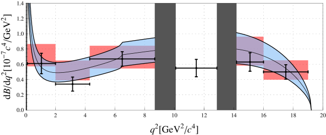
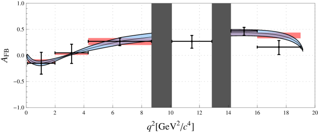
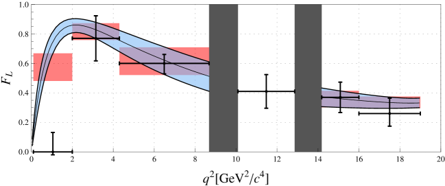
Figure 1: The SM predictions for the ${\rm d}\mathcal{B}/{\rm d}q^{2}$, $A_{\rm FB}$ and $F_{\rm L}$ with the theoretical uncertainties (the bands) versus the experimental measurements by LHCb [44]. The rate-averaged observables are indicated by the red regions.

For the decay $\bar{B}\to\bar{K}^{*}\mu^{+}\mu^{-}$, our SM predictions for the branching ratio ${\rm d}\mathcal{B}/{\rm d}q^{2}$, the forward-backward asymmetry $A_{\rm FB}$ and the longitudinal polarization fraction $F_{\rm L}$ with the available data from LHCb [44] are shown in figure 1. For the integrated observables, we take the ratio in eq. (3.2.2) after integrating its numerator and denominator separately. This definition agrees with the one used in the experimental measurements [28].

For the theoretical uncertainties, we follow closely the treatment of ref. [28]. At large recoil, we employ the naive factorization approach, therefore a real scale factor varying within $\pm 10\%$ is added to each of the transversity amplitudes $A_{\perp,\parallel,0}^{L,R}$ in eq. (B) to account for the $\mathcal{O}(\alpha_{s})$ and $\mathcal{O}(\Lambda/m_{b})$ subleading QCDF corrections. Similarly, at low recoil, the $\mathcal{O}(\alpha_{s}\Lambda/m_{b})$ subleading corrections to each of the transversity amplitudes $A_{\perp,\parallel,0}^{L,R}$ in eq. (B) are estimated by real scale factors varying within $\pm 5\%$. For the uncertainties due to the $\mathcal{O}(\Lambda/m_{b})$ subleading corrections to the improved Isgur-Wise relations and the $\mathcal{O}(m_{K^{*}}/m_{B})$ neglected kinematical factors, three real scale factors with $\pm 20\%$ uncertainties are assigned to the $\kappa C_{7}^{\rm eff}$ term for $A_{\perp,\parallel,0}^{L,R}$ in eq. (B), respectively. We obtain the theoretical uncertainties by varying each of the input parameters and the real scale factors mentioned above within its respective range and adding the individual uncertainty in quadrature.

From figure 1, it can be seen that the theoretical uncertainties for the branching ratio are about 30%, which mainly arise from the $B\to K^{*}$ form factors. However, in the angular observables forward-backward asymmetry and longitudinal fraction, these hadronic uncertainties cancel each other, which result in the relatively precise theoretical predictions.

With the theoretical uncertainties taken into account, the LHCb data are well consistent with the SM predictions except the $F_{\rm L}$ in the lowest-$q^{2}$ bin $q^{2}\in[0.10,2.00]\,{\rm GeV}^{2}$. For this bin, it is noted that the recent LHCb preliminary result of the $F_{\rm L}$ (with $\mathcal{L}=1\,{\rm fb}^{-1}$) [45] deviates from their previous result [44] by about $2.5\sigma$ and is in agreement with the SM prediction.

For the $B_{s}\to\mu^{+}\mu^{-}$ decay, with the up-to-date input parameters listed in table 1, we obtain the SM prediction

$$\overline{\mathcal{B}}(B_{s}\to\mu^{+}\mu^{-})=(3.71\pm 0.24)\times 10^{-9},$$ (4.1)

where the theoretical uncertainty is dominated by the decay constant $f_{B_{s}}$ and the CKM matrix elements. As pointed out in ref. [61, 62], the correction in eq. (3.7) gives a 10% enhancement of the branching ratio (compared with the one without the effects of $B_{s}^{0}-\bar{B}_{s}^{0}$ mixing). This value is in good agreement with the observed rate at the LHCb, which will put severe constraints on the anomalous $tcZ$ coupling as seen in the following analysis.

4.2 Constraining anomalous $tcZ$ coupling

In order to constrain the anomalous $tcZ$ coupling, we consider the SM predictions with $2\sigma$ error bars and the experimental data with $1\sigma$ error bar. For the $\bar{B}\to\bar{K}^{*}\mu^{+}\mu^{-}$ decays, as discussed in subsection 3.2.2 and 4.1, the LHCb data [44] in the following four bins $q^{2}\in[2.00,4.30]\,{\rm GeV}^{2}$, $[4.30,8.68]\,{\rm GeV}^{2}$, $[14.18,16.00]\,{\rm GeV}^{2}$ and $[16.00,19.00]\,{\rm GeV}^{2}$ are included in our analysis, which are also depicted in figure 1. For the decay $B_{s}\to\mu^{+}\mu^{-}$, we consider the recent LHCb measurements [46] listed in table 1.

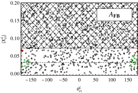
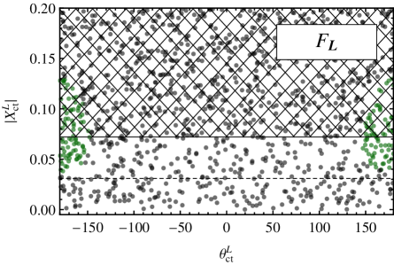
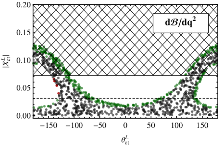
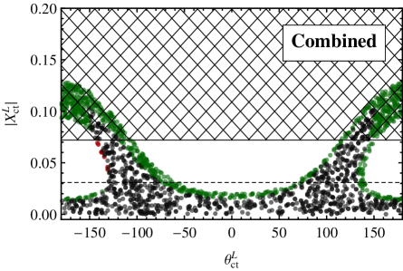
Figure 2: The allowed regions of the anomalous coupling $|X_{ct}^{L}|$ as a function of $\theta_{ct}^{L}$ under the constraints from $\bar{B}\to\bar{K}^{*}\mu^{+}\mu^{-}$ distributions ${\rm d}\mathcal{B}/{\rm d}q^{2}$, $A_{\rm FB}$ and $F_{\rm L}$ and their combinations by using the LHCb data [44]. The allowed regions by the experimental data at large recoil (low recoil) are shown in red and black (green and black) points. Furthermore, the black points are allowed by all the data. The cross-hatched region are excluded by the CMS bound on $\mathcal{B}(t\to cZ)$ [9]. The ATLAS $5\sigma$ discovery potential at $\mathcal{L}=10\;{\rm fb}^{-1}$ [10, 11] is indicated by the dashed line.

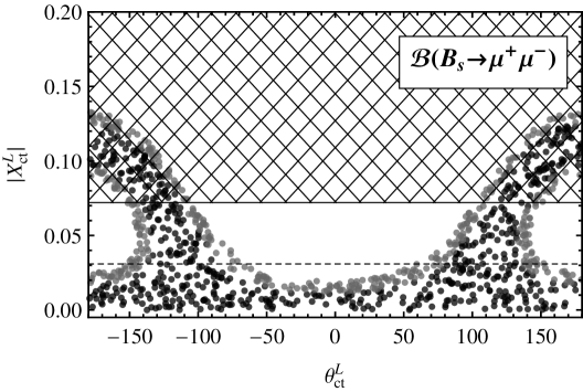
Figure 3: The upper bounds on the anomalous coupling $|X_{ct}^{L}|$ as a function of $\theta_{ct}^{L}$, constrained by the $\overline{\mathcal{B}}(B_{s}\to\mu^{+}\mu^{-})$. The black (gray and black) region are the allowed parameter space obtained with $1\sigma$ experimental error bar (the experimental true value interval at $90\%$ C.L.). The other captions are the same as in figure 2.

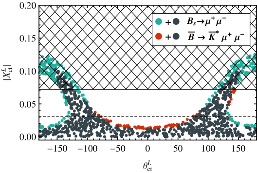
Figure 4: The combined upper bounds on the anomalous coupling $|X_{ct}^{L}|$ as a function of $\theta_{ct}^{L}$. The allowed regions by the experimental data of $B_{s}\to\mu^{+}\mu^{-}$ ($\bar{B}\to\bar{K}^{*}\mu^{+}\mu^{-}$) are indicated by both green and black (red and black) points. Furthermore, the black points are allowed by all the data. The other captions are the same as in figure 2.

The constraints on the anomalous coupling in the $|X_{ct}^{L}|-\theta_{ct}^{L}$ plane by the ${\rm d}\mathcal{B}/{\rm d}q^{2}$, $A_{\rm FB}$, $F_{\rm L}$ and their combinations in the $\bar{B}\to\bar{K}^{*}\mu^{+}\mu^{-}$ decays are shown in figure 2. It can be seen that, the potentially large $tcZ$ coupling effects are reflected in the stringent bound on its magnitude $|X_{ct}^{L}|$, which is currently dominated by the differential branching ratio. For a given value $|X_{ct}^{L}|$, the NP contribution is constructive to the SM one in the region $\theta_{ct}^{L}\approx 0^{\circ}$, whereas their interference becomes destructive in the region $\theta_{ct}^{L}\approx\pm 180^{\circ}$. Therefore, there are two favored solutions under the constraints of differential branching ratio in the $\theta_{ct}^{L}\approx\pm 180^{\circ}$ region. The solution with larger $|X_{ct}^{L}|$ corresponds to the case that the sign of $(C_{9}^{\rm eff},C_{10}^{\rm eff})$ has been flipped by the anomalous coupling. This solution is also not consistent with the CMS bound as depicted in figure 2. For the forward-backward asymmetry and longitudinal fraction, they can not provide strong constraints on the anomalous coupling. However, the longitudinal fraction at large recoil excludes this sign-flipped solution. Exploiting the $\bar{B}\to\bar{K}^{*}\mu^{+}\mu^{-}$ data, the constraints from the large recoil region are slightly more stringent than the ones from low recoil and comparable to the latter.

For the constraints on the anomalous $tcZ$ coupling by the $B_{s}\to\mu^{+}\mu^{-}$ decays, after considering the recent LHCb data [46], we update our previous results [24] at figure 3. It can be seen that, the interference structure between the SM and NP contributions manifested in the branching ratio is similar to the one in the $\bar{B}\to\bar{K}^{*}\mu^{+}\mu^{-}$ decays. Compared with our previous constraints, since the experimental data of $B_{s}\to\mu^{+}\mu^{-}$ are now double-bounded, it excludes parts of the parameter space in the destructive region $\theta_{ct}^{L}\approx\pm 180^{\circ}$ and leaves two solutions for $\lvert X_{ct}^{L}\rvert$.

The combined constraints obtained after considering all the experimental data of both $B_{s}\to\mu^{+}\mu^{-}$ and $\bar{B}\to\bar{K}^{*}\mu^{+}\mu^{-}$ decays are shown in figure 4. In the parameter space of ($\theta_{ct}^{L}$, $\lvert X_{ct}^{L}\rvert$), benefited from the angular observables, the $\bar{B}\to\bar{K}^{*}\mu^{+}\mu^{-}$ process excludes the regions corresponding to the sign-flipped solution. The constraints on the other part of the parameter space provided by these two decays are almost the same stringent. The detailed numerical results are listed in table 2. For general complex coupling $X_{ct}^{L}$, one can see that the predicted upper bound $\mathcal{B}(t\to cZ)<4.85\times 10^{-3}$ is compatible with the CMS direct bound $\mathcal{B}(t\to cZ)<2.4\times 10^{-3}$. For real coupling, the corresponding bound $\mathcal{B}(t\to cZ)<6.3\times 10^{-5}$ is below the CMS bound, but still of the same order as the $5\sigma$ discovery potential $\mathcal{B}(t\to cZ)\approx 4.4\times 10^{-4}$ of the LHC with an integrated luminosity of $10\,{\rm fb}^{-1}$.

	$\lvert X_{ct}^{L}\rvert$ constrained from			our bound
$\theta_{ct}^{L}$	$B_{s}\to\mu^{+}\mu^{-}$	$\bar{B}\to\bar{K}^{*}\mu^{+}\mu^{-}$	CMS	$\mathcal{B}(t\to cZ)$
$0^{\circ}$	$<0.012$	$<0.015$	$<0.072$	$<6.27\times 10^{-5}$
$180^{\circ}$	$<0.125$	$<0.013$	$<0.072$	$<0.75\times 10^{-4}$
$general$	$<0.125$	$<0.102$	$<0.072$	$<4.85\times 10^{-3}$

Table 2: The upper bounds on the magnitude $\lvert X_{ct}^{L}\rvert$ from the $\bar{B}\to\bar{K}^{*}\mu^{+}\mu^{-}$ and $B_{s}\to\mu^{+}\mu^{-}$ decays for some particular phases $\theta_{ct}^{L}$. The corresponding predicted bounds on $\mathcal{B}(t\to cZ)$ are also given. The bounds in the fourth column are obtained from the direct search of the $t\to cZ$ decay at the CMS [9].

5 Conclusions

In this paper, we have studied the effects of anomalous $tcZ$ coupling in the $\bar{B}\to\bar{K}^{*}\mu^{+}\mu^{-}$ decays at both the large and the low hadronic recoil region. With the recent LHCb measurements of $B_{s}\to\mu^{+}\mu^{-}$, the combined constraints on the anomalous coupling $X_{ct}^{L}$ from these two decays are derived. For general complex coupling, it is found that, the predicted upper limit of $\mathcal{B}(t\to cZ)$ is compatible with the CMS direct search. In particular, for real coupling, the corresponding limit is below the current CMS bound, but still stays in the accessible level of the LHC with an integrated luminosity of $10\;{\rm fb}^{-1}$.

It has been shown that, the $B_{s}\to\mu^{+}\mu^{-}$ and $\bar{B}\to\bar{K}^{*}\mu^{+}\mu^{-}$ decays can provide complementary information about the anomalous $tcZ$ coupling, and therefore they are correlated with the rare $t\to cZ$ decays. With improved measurements from the LHCb and the future super-B factories, these interplays will be enhanced and complementary to the direct search for the FCNC transitions in top quark decays performed at the LHC CMS and ATLAS experiments.

Appendix A The form factors

For the $\bar{B}\to\bar{K}^{*}$ transitions, we can use seven QCD form factors parameterize the matrix elements of $\mathcal{O}_{7,9,10}$ as ($q^{\mu}=p^{\mu}-k^{\mu}$) [79]

$$\langle\bar{K}^{*}(k,\epsilon)|\bar{s}\gamma_{\mu}(1-\gamma_{5})b|\bar{B}(p)\rangle= -i\epsilon_{\mu}^{*}(m_{B}+m_{K^{*}})A_{1}(q^{2})+i(2p-q)_{\mu}(\epsilon^{*}\cdot q)\frac{A_{2}(q^{2})}{m_{B}+m_{K^{*}}}$$

$$+iq_{\mu}(\epsilon^{*}\cdot q)\frac{2m_{K*}}{q^{2}} [A_{3}(q^{2})-A_{0}(q^{2})]+\epsilon_{\mu\nu\rho\sigma}\epsilon^{*\nu}p^{\rho}k^{\sigma}\frac{2V(q^{2})}{m_{B}+m_{K^{*}}},$$

$$\langle\bar{K}^{*}(k,\epsilon)|\bar{s}\sigma_{\mu\nu}q^{\nu}(1+\gamma_{5})b|\bar{B}(p)\rangle =+T_{3}(q^{2})(\epsilon^{*}\cdot q)\left[q_{\mu}-\frac{q^{2}}{m_{B}^{2}-m_{K^{*}}^{2}}(2p-q)_{\mu}\right]$$

$$+i\epsilon_{\mu\nu\rho\sigma}\epsilon^{*\nu}p^{\rho}k^{\sigma}2T_{1}( q^{2})+T_{2}(q^{2})\left[\epsilon_{\mu}^{*}(m_{B}^{2}-m_{K^{*}}^{2})-(\epsilon^{*}\cdot q)(2p-q)_{\mu}\right],$$ (A.1)

with

$$A_{3}(q^{2})=\frac{m_{B}+m_{K^{*}}}{2m_{K^{*}}}A_{1}(q^{2})-\frac{m_{B}-m_{K^{*}}}{2m_{K^{*}}}A_{2}(q^{2})$$ (A.2)

and

$$A_{0}(0)=A_{3}(0),\qquad\qquad T_{1}(0)=T_{2}(0).$$ (A.3)

At large recoil, after adopting the QCDF approach [80], these seven form factors can be reduced to two universal form factors, which are related to the form factors $V,A_{1,2}$ as [81, 27]

$$\xi_{\perp}(q^{2})=\frac{m_{B}}{m_{B}+m_{K^{*}}}V(q^{2}),\qquad\xi_{\parallel}(q^{2})=\frac{m_{B}+m_{K^{*}}}{2E_{K^{*}}}A_{1}(q^{2})-\frac{m_{B}-m_{K^{*}}}{m_{B}}A_{2}(q^{2}).$$ (A.4)

At low recoil, the improved Isgur-Wise relations imply the vector and tensor form factors are connected as follows to leading order in $1/m_{b}$ [66, 67],

$$T_{1}(q^{2})=\kappa V(q^{2}),\qquad T_{2}(q^{2})=\kappa A_{1}(q^{2}),\qquad T_{3}(q^{2})=\kappa A_{2}(q^{2})\frac{m_{B}^{2}}{q^{2}},$$ (A.5)

with

$$\kappa=1-\frac{2\alpha_{s}}{3\pi}\ln\left(\frac{\mu}{m_{b}}\right),$$ (A.6)

after neglecting subleading terms.

For the $B\to K^{*}$ form factors $V,A_{1,2}$, we adopt results of light-cone sum rule approach [79]

$$V(q^{2}) =\frac{r_{1}}{1-q^{2}/m_{R}^{2}}+\frac{r_{2}}{1-q^{2}/m_{\rm fit}^{2}}, {\rm with}\;r_{1} =0.923,r_{2}=-0.511,$$

$$m_{R} =5.32\,{\rm GeV},m_{\rm fit}^{2}=49.40\,{\rm GeV^{2}},$$

$$A_{1}(q^{2}) =\frac{r_{2}}{1-q^{2}/m_{\rm fit}^{2}}, {\rm with}\;r_{2} =0.290,m_{\rm fit}^{2}=40.38\,{\rm GeV^{2}},$$

$$A_{2}(q^{2}) =\frac{r_{1}}{1-q^{2}/m_{\rm fit}^{2}}+\frac{r_{2}}{(1-q^{2}/m_{\rm fit})^{2}}, {\rm with}\;r_{1} =-0.084,r_{2}=0.342,m_{\rm fit}^{2}=52.00\,{\rm GeV^{2}}.$$ (A.7)

Their relative uncertainties at $q^{2}=0$ are $\delta V(0)=\pm 11\%$, $\delta A_{1}(0)=\pm 12\%$ and $\delta A_{2}(0)=\pm 13\%$ after taking into account the uncertainties induced by the Gegenbauer moment $a_{1,K^{*}}$. For the $q^{2}>0$ region, the relative uncertainties are estimated to be the same as the ones at $q^{2}=0$.

Appendix B The transversity amplitudes

For the theoretical framework at the large and the low hadronic recoil region, we follow closely the ref. [82, 28] and recapitulate the relevant formulae in the following.

The transversity amplitudes at large recoil

At large recoil, application of QCDF yields the following transversity amplitudes [82]

$$A_{\perp}^{L,R} =+\sqrt{2}Nm_{B}(1-\hat{s})\left[\bigl{(}\mathcal{C}_{9}\mp\mathcal{C}_{10}\bigr{)}\xi_{\perp}+\frac{2\hat{m}_{b}}{\hat{s}}\mathcal{T}_{\perp}^{+}\right],$$

$$A_{\parallel}^{L,R} =-\sqrt{2}Nm_{B}(1-\hat{s})\left[\bigl{(}\mathcal{C}_{9}\mp\mathcal{C}_{10}\bigr{)}\xi_{\perp}+\frac{2\hat{m}_{b}}{\hat{s}}\mathcal{T}_{\perp}^{-}\right],$$

$$A_{0}^{L,R} =-\frac{Nm_{B}^{2}(1-\hat{s})^{2}}{2m_{K^{*}}\sqrt{\hat{s}}}\biggl{[}\bigl{(}\mathcal{C}_{9}\mp\mathcal{C}_{10}\bigr{)}\xi_{\parallel}-2\hat{m}_{b}\mathcal{T}_{\parallel}^{-}\biggr{]},$$ (B.1)

where

$$\quad\hat{s}=\frac{q^{2}}{m_{B}^{2}},\qquad\hat{m}_{b}=\frac{m_{b}}{m_{B}},\qquad\hat{m}_{K^{*}}=\frac{m_{K^{*}}}{m_{B}},\qquad N=\left[\frac{G_{F}^{2}\alpha_{e}^{2}|\lambda_{t}|^{2}}{3\cdot 2^{10}\pi^{5}}m_{B}\hat{s}\sqrt{\hat{\lambda}}\beta_{l}\right]^{1/2},$$

$$\mathcal{C}_{9,10}=\frac{4\pi}{\alpha_{s}}C_{9,10},\qquad\hat{\lambda}=1+\hat{m}_{K^{*}}^{4}+\hat{s}^{2}-2(\hat{m}_{K^{*}}^{2}+\hat{s}+\hat{s}\hat{m}_{K^{*}}^{2}).\quad\quad\quad$$ (B.2)

The functions $\mathcal{T}_{\perp,\parallel}^{\pm}$ have been calculated at NLO [26, 27], which have the following general structure

$$\mathcal{T}_{a}^{\pm} =\mathcal{T}_{a}^{\pm(t)}+\hat{\lambda}_{u}\mathcal{T}_{a}^{(u)}, \mathcal{T}_{a}^{\pm(t)} =\mathcal{T}_{a}^{\pm(t),{\rm LO}}+\frac{\alpha_{s}}{4\pi}\mathcal{T}_{a}^{\pm(t),{\rm NLO}},$$

$$\hat{\lambda}_{u} =\frac{V_{ub}V_{us}^{*}}{V_{tb}V_{ts}^{*}}, \mathcal{T}_{a}^{(u)} =\mathcal{T}_{a}^{(u),{\rm LO}}+\frac{\alpha_{s}}{4\pi}\mathcal{T}_{a}^{(u),{\rm NLO}},$$ (B.3)

where $a=\perp,\parallel$. The LO formulae read

$$\mathcal{T}_{\perp}^{\pm(t),{\rm LO}} =+\xi_{\perp}\left(C_{7}^{\rm eff(0)}+\frac{\hat{s}}{2\hat{m}_{b}}Y^{(0)}\right), \mathcal{T}_{\perp}^{(u),{\rm LO}} =+\xi_{\perp}\frac{\hat{s}}{2\hat{m}_{b}}Y^{(u)(0)},$$

$$\mathcal{T}_{\parallel}^{-(t),{\rm LO}} =-\xi_{\parallel}\left(C_{7}^{\rm eff(0)}+\frac{1}{2\hat{m}_{b}}Y^{(0)}\right)+HS, \mathcal{T}_{\parallel}^{(u),{\rm LO}} =-\xi_{\parallel}\frac{1}{2\hat{m}_{b}}Y^{(u)(0)}+HS,$$ (B.4)

where spectator effects are denoted by $HS$. The functions involving the one-loop contributions of four-quark operators are defined as

$$Y(q^{2})= +h(q^{2},m_{c})\left(\frac{4}{3}C_{1}+C_{2}+6C_{3}+60C_{5}\right)-\frac{1}{2}h(q^{2},m_{b})\left(7C_{3}+\frac{4}{3}C_{4}+76C_{5}+\frac{64}{3}C_{6}\right)$$

$$-\frac{1}{2}h(q^{2},0)\left(C_{3}+\frac{4}{3}C_{4}+16C_{5}+\frac{64}{3}C_{6}\right)+\frac{4}{3}C_{3}+\frac{64}{9}C_{5}+\frac{64}{27}C_{6},$$

$$Y^{(u)}(q^{2})= +\left(\frac{4}{3}C_{1}+C_{2}\right)\left[h(q^{2},m_{c})-h(q^{2},0)\right].$$ (B.5)

The basic fermion loop function reads

$$h(q^{2},m_{q})=-\frac{4}{9}\left(\ln\frac{m_{q}^{2}}{\mu^{2}}-\frac{2}{3}-z\right)-\frac{4}{9}(2+z)\sqrt{|z-1|}\times\begin{cases}\arctan\frac{1}{\sqrt{z-1}}&z>1\\ \ln{\frac{1+\sqrt{1-z}}{\sqrt{z}}}-\frac{i\pi}{2}&z\leq 1\end{cases}$$ (B.6)

with $z=4m_{q}^{2}/q^{2}$.

The transversity amplitudes at low recoil

At low recoil, with the improved Isgur-Wise form factor relations eq. (A.5), the transversity amplitudes can be written as [28]

$$A_{\perp}^{L,R} =+i\left[\left(C_{9}^{\rm eff}\mp C_{10}^{\rm eff}\right)+\kappa\frac{2\hat{m}_{b}}{\hat{s}}C_{7}^{\rm eff}\right]f_{\perp},$$

$$A_{\parallel}^{L,R} =-i\left[\left(C_{9}^{\rm eff}\mp C_{10}^{\rm eff}\right)+\kappa\frac{2\hat{m}_{b}}{\hat{s}}C_{7}^{\rm eff}\right]f_{\parallel},$$

$$A_{0}^{L,R} =-i\left[\left(C_{9}^{\rm eff}\mp C_{10}^{\rm eff}\right)+\kappa\frac{2\hat{m}_{b}}{\hat{s}}C_{7}^{\rm eff}\right]f_{0},$$ (B.7)

with the definitions

$$N =\left[\frac{G_{F}^{2}\alpha_{e}^{2}|\lambda_{t}|^{2}}{3\cdot 2^{10}\pi^{5}}m_{B}\hat{s}\sqrt{\hat{\lambda}}\right]^{\rm 1/2}, \quad f_{\parallel} =Nm_{B}\sqrt{2}(1+\hat{m}_{K^{*}})A_{1}(q^{2}),$$

$$f_{0} =Nm_{B}\frac{(1-\hat{s}-\hat{m}_{K^{*}}^{2})(1+\hat{m}_{K^{*}})^{2}A_{1}(q^{2})-\hat{\lambda}A_{2}(q^{2})}{2\hat{m}_{K^{*}}(1+\hat{m}_{K^{*}})\sqrt{\hat{s}}}, \quad f_{\perp} =Nm_{B}\frac{\sqrt{2\hat{\lambda}}}{1+\hat{m}_{K^{*}}}V(q^{2}).$$ (B.8)

Furthermore, we can define the two independent combinations of Wilson coefficients as [28]

$$\rho_{1}\equiv\left|C_{9}^{\rm eff}+\kappa\frac{2\hat{m}_{b}}{\hat{s}}C_{7}^{\rm eff}\right|^{2}+\left|C_{10}^{\rm eff}\right|^{2},\qquad\rho_{2}\equiv{\rm Re}\left\{\left(C_{9}^{\rm eff}+\kappa\frac{2\hat{m}_{b}}{\hat{s}}C_{7}^{\rm eff}\right)C_{10}^{{\rm eff}*}\right\}.$$ (B.9)

Then, at low recoil, the observables in eq. (3.2.2) turn to be the transparent forms

$$\frac{{\rm d}\Gamma}{{\rm d}q^{2}}=2\rho_{1}\times(f_{0}^{2}+f_{\perp}^{2}+f_{\parallel}^{2}),\quad A_{\rm FB}=3\frac{\rho_{2}}{\rho_{1}}\times\frac{f_{\perp}f_{\parallel}}{f_{0}^{2}+f_{\perp}^{2}+f_{\parallel}^{2}},\quad F_{\rm L}=\frac{f_{0}^{2}}{f_{0}^{2}+f_{\perp}^{2}+f_{\parallel}^{2}}.$$ (B.10)

References

- [1] S. L. Glashow, J. Iliopoulos and L. Maiani, Phys. Rev. D 2, 1285 (1970).
- [2] G. Eilam, J. L. Hewett and A. Soni, Phys. Rev. D 44, 1473 (1991) [Erratum-ibid. D 59, 039901 (1999)].
- [3] J. A. Aguilar-Saavedra, Acta Phys. Polon. B 35, 2695 (2004) [hep-ph/0409342].
- [4] M. Beneke, I. Efthymiopoulos, M. L. Mangano, J. Womersley, A. Ahmadov, G. Azuelos, U. Baur and A. Belyaev et al., In *Geneva 1999, Standard model physics (and more) at the LHC* 419-529 [hep-ph/0003033].
- [5] W. Bernreuther, J. Phys. G 35, 083001 (2008) [arXiv:0805.1333 [hep-ph]].
- [6] T. Aaltonen et al. [CDF Collaboration], Phys. Rev. Lett. 101, 192002 (2008) [arXiv:0805.2109 [hep-ex]].
- [7] V. M. Abazov et al. [D0 Collaboration], Phys. Lett. B 701 (2011) 313 [arXiv:1103.4574 [hep-ex]].
- [8] G. Aad et al. [ATLAS Collaboration], JHEP 1209, 139 (2012) [arXiv:1206.0257 [hep-ex]].
- [9] S. Chatrchyan et al. [CMS Collaboration], arXiv:1208.0957 [hep-ex].
- [10] J. Carvalho et al. [ATLAS Collaboration], Eur. Phys. J. C 52, 999 (2007) [arXiv:0712.1127 [hep-ex]].
- [11] F. M. A. Veloso, CERN-THESIS-2008-106.
- [12] L. Benucci and A. Kyriakis, Nucl. Phys. Proc. Suppl. 177-178, 258 (2008).
- [13] T. Han, K. Whisnant, B. L. Young and X. Zhang, Phys. Rev. D 55, 7241 (1997) [hep-ph/9603247].
- [14] T. Han, K. Whisnant, B. L. Young and X. Zhang, Phys. Lett. B 385, 311 (1996) [hep-ph/9606231].
- [15] F. Larios, M. A. Perez and C. P. Yuan, Phys. Lett. B 457, 334 (1999) [hep-ph/9903394].
- [16] G. Burdman, M. C. Gonzalez-Garcia and S. F. Novaes, Phys. Rev. D 61, 114016 (2000) [hep-ph/9906329].
- [17] P. J. Fox, Z. Ligeti, M. Papucci, G. Perez and M. D. Schwartz, Phys. Rev. D 78, 054008 (2008) [arXiv:0704.1482 [hep-ph]].
- [18] J. P. Lee and K. Y. Lee, Phys. Rev. D 78, 056004 (2008) [arXiv:0806.1389 [hep-ph]].
- [19] J. Drobnak, S. Fajfer and J. F. Kamenik, Phys. Lett. B 701, 234 (2011) [arXiv:1102.4347 [hep-ph]].
- [20] J. Drobnak, S. Fajfer and J. F. Kamenik, Nucl. Phys. B 855, 82 (2012) [arXiv:1109.2357 [hep-ph]].
- [21] B. Grzadkowski and M. Misiak, Phys. Rev. D 78, 077501 (2008) [Erratum-ibid. D 84, 059903 (2011)] [arXiv:0802.1413 [hep-ph]].
- [22] X. Yuan, Y. Hao and Y. Yang, Phys. Rev. D 83, 013004 (2011) [arXiv:1010.1912 [hep-ph]].
- [23] X. -Q. Li, Y. -D. Yang and X. -B. Yuan, JHEP 1108, 075 (2011) [arXiv:1105.0364 [hep-ph]].
- [24] X. -Q. Li, Y. -D. Yang and X. -B. Yuan, JHEP 1203, 018 (2012) [arXiv:1112.2674 [hep-ph]].
- [25] A. Ali, P. Ball, L. T. Handoko and G. Hiller, Phys. Rev. D 61, 074024 (2000) [hep-ph/9910221].
- [26] M. Beneke, T. Feldmann and D. Seidel, Nucl. Phys. B 612, 25 (2001) [hep-ph/0106067].
- [27] M. Beneke, T. .Feldmann and D. Seidel, Eur. Phys. J. C 41, 173 (2005) [hep-ph/0412400].
- [28] C. Bobeth, G. Hiller and D. van Dyk, JHEP 1007, 098 (2010) [arXiv:1006.5013 [hep-ph]].
- [29] A. Khodjamirian, T. .Mannel, A. A. Pivovarov and Y. -M. Wang, JHEP 1009, 089 (2010) [arXiv:1006.4945 [hep-ph]].
- [30] A. Khodjamirian, T. .Mannel and Y. -M. Wang, JHEP 1302, 010 (2013) [arXiv:1211.0234 [hep-ph]].
- [31] F. Kruger and J. Matias, Phys. Rev. D 71, 094009 (2005) [hep-ph/0502060].
- [32] Q. Chang, X. -Q. Li and Y. -D. Yang, JHEP 1004, 052 (2010) [arXiv:1002.2758 [hep-ph]].
- [33] W. Altmannshofer, P. Paradisi and D. M. Straub, JHEP 1204, 008 (2012) [arXiv:1111.1257 [hep-ph]].
- [34] R. -M. Wang, Y. -G. Xu, Y. -L. Wang and Y. -D. Yang, Phys. Rev. D 85, 094004 (2012) [arXiv:1112.3174 [hep-ph]].
- [35] F. Beaujean, C. Bobeth, D. van Dyk and C. Wacker, JHEP 1208, 030 (2012) [arXiv:1205.1838 [hep-ph]].
- [36] F. Kruger, L. M. Sehgal, N. Sinha and R. Sinha, Phys. Rev. D 61, 114028 (2000) [Erratum-ibid. D 63, 019901 (2001)] [hep-ph/9907386].
- [37] C. S. Kim, Y. G. Kim, C. -D. Lu and T. Morozumi, Phys. Rev. D 62, 034013 (2000) [hep-ph/0001151].
- [38] S. Descotes-Genon, J. Matias, M. Ramon and J. Virto, arXiv: 1207.2753 [hep-ph];
- [39] J. Matias, F. Mescia, M. Ramon and J. Virto, arXiv: 1202.4266 [hep-ph].
- [40] J. P. Lees et al. [BABAR Collaboration], Phys. Rev. D 86, 032012 (2012) [arXiv:1204.3933 [hep-ex]].
- [41] J. -T. Wei et al. [BELLE Collaboration], Phys. Rev. Lett. 103, 171801 (2009) [arXiv:0904.0770 [hep-ex]].
- [42] T. Aaltonen et al. [CDF Collaboration], Phys. Rev. Lett. 108, 081807 (2012) [arXiv:1108.0695 [hep-ex]].
- [43] Hideki Miyake for the CDF Collaboration, presented at ICHEP, July 2012, slides available at http://indico.cern.ch/contributionDisplay.py?contribId=502&confId=181298.
- [44] RAaij et al. [LHCb Collaboration], Phys. Rev. Lett. 108, 181806 (2012) [arXiv:1112.3515 [hep-ex]].
- [45] Abraham Gallas for the LHCb Collaboration, presented at ICHEP, July 2012, slides available at http://indico.cern.ch/contributionDisplay.py?contribId=560&confId=181298.
- [46] RAaij et al. [LHCb Collaboration], arXiv:1211.2674 .
- [47] T. Appelquist and J. Carazzone, Phys. Rev. D 11, 2856 (1975).
- [48] W. Buchmuller and D. Wyler, Nucl. Phys. B 268, 621 (1986).
- [49] B. Grzadkowski, M. Iskrzynski, M. Misiak and J. Rosiek, JHEP 1010, 085 (2010) [arXiv:1008.4884 [hep-ph]].
- [50] W. Hollik, J. I. Illana, S. Rigolin, C. Schappacher and D. Stockinger, Nucl. Phys. B 551, 3 (1999) [Erratum-ibid. B 557, 407 (1999)] [hep-ph/9812298].
- [51] J. A. Aguilar-Saavedra, Nucl. Phys. B 812, 181 (2009) [arXiv:0811.3842 [hep-ph]].
- [52] K. G. Chetyrkin, M. Misiak and M. Munz, Phys. Lett. B 400, 206 (1997) [Erratum-ibid. B 425, 414 (1998)] [hep-ph/9612313].
- [53] C. Bobeth, M. Misiak and J. Urban, Nucl. Phys. B 574, 291 (2000) [hep-ph/9910220].
- [54] P. Gambino, M. Gorbahn and U. Haisch, Nucl. Phys. B 673, 238 (2003) [hep-ph/0306079].
- [55] M. Gorbahn and U. Haisch, Nucl. Phys. B 713, 291 (2005) [hep-ph/0411071].
- [56] M. Gorbahn, U. Haisch and M. Misiak, Phys. Rev. Lett. 95, 102004 (2005) [hep-ph/0504194].
- [57] A. J. Buras, M. Misiak, M. Munz and S. Pokorski, Nucl. Phys. B 424, 374 (1994) [hep-ph/9311345].
- [58] G. Buchalla and A. J. Buras, Nucl. Phys. B 548, 309 (1999) [hep-ph/9901288].
- [59] M. Misiak and J. Urban, Phys. Lett. B 451, 161 (1999) [hep-ph/9901278].
- [60] A. J. Buras, J. Girrbach, D. Guadagnoli and G. Isidori, Eur. Phys. J. C 72, 2172 (2012) [arXiv:1208.0934 [hep-ph]].
- [61] K. De Bruyn, R. Fleischer, R. Knegjens, P. Koppenburg, M. Merk, A. Pellegrino and N. Tuning, Phys. Rev. Lett. 109, 041801 (2012) [arXiv:1204.1737 [hep-ph]].
- [62] K. De Bruyn, R. Fleischer, R. Knegjens, P. Koppenburg, M. Merk and N. Tuning, Phys. Rev. D 86, 014027 (2012) [arXiv:1204.1735 [hep-ph]].
- [63] RAaij et al. [LHCb Collaboration], LHCb-CONF-2012-002
- [64] G. Buchalla and G. Isidori, Nucl. Phys. B 525, 333 (1998) [hep-ph/9801456].
- [65] M. Beylich, G. Buchalla and T. Feldmann, Eur. Phys. J. C 71, 1635 (2011) [arXiv:1101.5118 [hep-ph]].
- [66] B. Grinstein and D. Pirjol, Phys. Lett. B 533, 8 (2002) [hep-ph/0201298].
- [67] B. Grinstein and D. Pirjol, Phys. Rev. D 70, 114005 (2004) [hep-ph/0404250].
- [68] M. Beneke, G. Buchalla, M. Neubert and C. T. Sachrajda, Eur. Phys. J. C 61, 439 (2009) [arXiv:0902.4446 [hep-ph]].
- [69] W. Altmannshofer, P. Ball, A. Bharucha, A. J. Buras, D. M. Straub and M. Wick, JHEP 0901, 019 (2009) [arXiv:0811.1214 [hep-ph]].
- [70] T. Han, R. D. Peccei and X. Zhang, Nucl. Phys. B 454, 527 (1995) [hep-ph/9506461].
- [71] J. J. Zhang, C. S. Li, J. Gao, H. Zhang, Z. Li, C. -P. Yuan and T. -C. Yuan, Phys. Rev. Lett. 102, 072001 (2009) [arXiv:0810.3889 [hep-ph]].
- [72] J. Drobnak, S. Fajfer and J. F. Kamenik, Phys. Rev. Lett. 104, 252001 (2010) [arXiv:1004.0620 [hep-ph]].
- [73] J. J. Zhang, C. S. Li, J. Gao, H. X. Zhu, C. -P. Yuan and T. -C. Yuan, Phys. Rev. D 82, 073005 (2010) [arXiv:1004.0898 [hep-ph]].
- [74] J. Drobnak, S. Fajfer and J. F. Kamenik, Phys. Rev. D 82, 073016 (2010) [arXiv:1007.2551 [hep-ph]].
- [75] J. Beringer et al. [Particle Data Group Collaboration], Phys. Rev. D 86, 010001 (2012).
- [76] J. Charles et al. [CKMfitter Group Collaboration], Eur. Phys. J. C 41, 1 (2005) [hep-ph/0406184], updated results and plots available at: http://ckmfitter.in2p3.fr
- [77] T. Aaltonen et al. [CDF and D0 Collaborations], Phys. Rev. D 86, 092003 (2012) [arXiv:1207.1069 [hep-ex]].
- [78] J. Laiho, E. Lunghi and R. S. Van de Water, Phys. Rev. D 81, 034503 (2010) [arXiv:0910.2928 [hep-ph]]. Updates available on http://latticeaverages.org/.
- [79] P. Ball and R. Zwicky, Phys. Rev. D 71, 014015 (2005) [hep-ph/0406232]. P. Ball and R. Zwicky, Phys. Rev. D 71, 014029 (2005) [hep-ph/0412079].
- [80] J. Charles, A. Le Yaouanc, L. Oliver, O. Pene and J. C. Raynal, Phys. Rev. D 60, 014001 (1999) [hep-ph/9812358].
- [81] M. Beneke and T. Feldmann, Nucl. Phys. B 592, 3 (2001) [hep-ph/0008255].
- [82] C. Bobeth, G. Hiller and G. Piranishvili, JHEP 0807, 106 (2008) [arXiv:0805.2525 [hep-ph]].