Adaptive propagation of quantum few-body systems with time-dependent Hamiltonians

Abstract

In this study, a variety of methods are tested and compared for the numerical solution of the Schrödinger equation for few-body systems with explicitely time-dependent Hamiltonians, with the aim to find the optimal one. The configuration interaction method, generally applied to find stationary eigenstates accurately and without approximations to the wavefunction’s structure, may also be used for the time-evolution, which results in a large linear system of ordinary differential equations. The large basis sizes typically present when the configuration interaction method is used calls for efficient methods for the time evolution. Apart from efficiency, adaptivity (in the time domain) is the other main focus in this study, such that the time step is adjusted automatically given some requested accuracy. A method is suggested here, based on an exponential integrator approach, combined with different ways to implement the adaptivity, which was found to be faster than a broad variety of other methods that were also considered.

Mathematical Physics, LTH, Lund University, SE-22100 Lund, Sweden

1 Introduction

Experimental development in recent years has allowed for creation and detailed control of tunable quantum mechanical few-body systems. For example, trapped ultra-cold atomic or molecular gases are systems where both trapping potentials and the particle-particle interactions may be directly controlled via externally applied fields [1, 2, 3, 4, 5], and such systems have also been realized with very few particles [4, 6]. Another example is electrons confined in so-called quantum dots, small semiconductor based structures, where for example electric and magnetic fields also can be used to affect the particles [7, 8, 9]. Such systems can allow for the study of, for example, non-equilibrium time-dependent processes, quantum quenches, or laser-induced dynamics, with strongly interacting particles.

In this study, a variety of numerical methods have been tested, to simulate the time-evolution of such systems as efficiently as possible. A method based on an exponential-integrator approach was found to be the most efficient. It re-uses some important concepts from one presented in a work by Park and Light [10], but is here extended to handle also time-dependent Hamiltonians, by implementing the time-adaptivity in a different way.

The methods are described in section 2. Then a physical test case, along with the numerical performance tests, is presented in section 3. A summary is given in section 4, and the appendix contains some remarks on the implementation, along with a short discussion about some other methods.

2 Method

The configuration interaction method (or “exact diagonalization”) is widely used to model quantum mechanical few-body systems. Its versatility allows its usage in different fields such as quantum chemistry, nuclear physics, and condensed matter physics (see for example Refs. [11, 12, 13]). In practice the method is limited to very small numbers of particles, but its advantages are that it does not involve any initial assumptions about the structure of the many-body wavefunction, and it is fully capable to describe also excited states. Furthermore, it is rather flexible in the sense that it can handle both bosons and fermions, and is not restricted to any particular kind of interaction between the particles. While typically employed to find eigenstates for the time-independent Schrödinger equation, it can also be used as a foundation for solving the time-dependent one,

$$\frac{d}{dt}|\Psi(t)\rangle=-iH(t)|\Psi(t)\rangle$$ (1)

with some initial state $|\Psi(0)\rangle$. (Throughout this paper we set $\hbar=1$.) The states are expanded as linear combinations of some set of (static) many-body basis states, denoted by $|\Phi_{\nu}\rangle$ below. Eigenstates of a Hamiltonian may be obtained by finding eigenvectors of its matrix representation in the given basis. For many typical cases this matrix is very sparse. For a state $|\Psi(t)\rangle$ that changes in time, the time-dependence is contained in the coefficients $b_{\nu}(t)$ of the expansion:

$$|\Psi(t)\rangle=\sum_{\nu}b_{\nu}(t)|\Phi_{\nu}\rangle$$ (2)

With this expansion inserted in Eq. (1), it yields a system of linearly coupled ordinary differential equations for the coefficients $b_{\nu}(t)$. There is then a variety of numerical approaches that can be used to solve it, although the large dimensionality of typical problems makes it crucial to work with efficient methods. Within this study several options have been compared, in an attempt to find the optimal one, for the systems intended to be investigated. For example, standard Runge-Kutta methods, explicit or implicit, may be used. However, another class of methods, generally referred to as exponential integrators (described in the following sections), have in many cases been found to be more efficient for the problem at hand [14].

A number of earlier studies have utilized time-dependent configuration interaction methods, in particular to study electronic response to applied laser fields (see, for example, Refs. [15, 16, 17, 18, 19, 20, 21]). Typically in this context, a Hartree-Fock solution together with single particle-hole excitations is used to model the excitation of an atom or molecule by a light field. Some other recent studies suggest and use time-dependent methods specialized for interacting bosons, such as a multiconfigurational Hartree method [23], or, in another study, a method employing time-dependent basis states, which results in a set of nonlinear equations [22]. In the present study, however, the wish is to handle systems with as general time-dependent Hamiltonians as possible, including time-dependent interactions, and the possibility for both bosons and fermions.

The methods tested here are described in the sections below: Section 2.1 describes propagation of constant (time-independent) Hamiltonians, closely following the approach by Park and Light [10]. But for time-dependent Hamiltonians, a different method (in two variants) is suggested and tested in this study, described in section 2.2. A high-order Runge-Kutta method is also considered here, described in section 2.3. Initially in this project, an implicit method was also tested but found to be inefficient, details about this are given in section A.2 of the appendix.

2.1 Adaptive Lanczos propagation with a constant Hamiltonian (ALC)

If the Hamiltonian $H$ in Eq. (1) does not depend on time, then a formal solution is given by

$$|\Psi(t)\rangle=\exp(-itH)|\Psi(0)\rangle$$ (3)

with a so-called exponential integrator. Because of the large dimensions of the Hilbert spaces considered here, it is not feasible to directly compute the whole matrix exponential. Instead, the Lanczos process [24, 25] can be used to create an approximation for $H$, which may then be used to compute the evolution during a small time step $\Delta t$, and this scheme is then iterated several times. This approach was presented in a work by Park and Light [10]. The method, with a small modification, is described in detail below since its main concepts are relevant also for time-dependent Hamiltonians, as discussed in the next section. For a more mathematical perspective on exponential integrators, see for example Refs. [26, 27, 28, 29].

It should be noted here that even if the method below is only applicable for Hamiltonians without an explicit time-dependence, it can of course be readily applied to any piece-wise constant Hamiltonian by separating the time axis into appropriate subintervals.

The Lanczos process, truncated after some finite number of iterations, yields an orthogonal set of vectors in a matrix $K$, the Krylov space, coupled by a tridiagonal matrix $T$ [24, 25]:

$$H=KTK^{\dagger}=\left[\begin{array}[]{cccc}|&|&|\\ |k_{0}\rangle&|k_{1}\rangle&|k_{2}\rangle&\cdots\\ |&|&|\end{array}\right]\left[\begin{array}[]{cccc}\alpha_{0}&\beta_{0}&0&0\\ \beta_{0}&\alpha_{1}&\beta_{1}&0\\ 0&\beta_{1}&\alpha_{2}&\ddots\\ 0&0&\ddots&\ddots\end{array}\right]\left[\begin{array}[]{ccc}-&|k_{0}\rangle^{\dagger}&-\\ -&|k_{1}\rangle^{\dagger}&-\\ -&|k_{2}\rangle^{\dagger}&-\\ &\vdots\end{array}\right]$$ (4)

The first vector $|k_{0}\rangle$ is just $|\Psi(t_{0})\rangle$, and $t_{0}$ is the time at the beginning of the small time step. Then, the next vector $|k_{1}\rangle$ is obtained by applying $H$ on $|k_{0}\rangle$ and projecting out the component along $|k_{0}\rangle$, to make $|k_{1}\rangle$ orthogonal to $|k_{0}\rangle$, and similarly for subsequent vectors. Only matrix-vector products are required, no other manipulation of $H$ is needed, making this approach useful for sparse matrices. By inserting the factorization above into Eq. (3), together with a diagonalization $T=QDQ^{\dagger}$, we get

$$|\Psi(t_{0}+\Delta t)\rangle=KQe^{-i\Delta tD}Q^{\dagger}K^{\dagger}|\Psi(t_{0})\rangle$$ (5)

As $D$ is diagonal, it can be exponentiated trivially, and $|\Psi(t_{0}+\Delta t)\rangle$ can be computed.

It remains however to choose the dimension $d_{K}$ of the Krylov space, and the time step $\Delta t$. The approach here is very similar to the one described in Ref. [10] for $\Delta t$. With a closer look at Eq. (5), one may view the expression as a differential equation “within the Krylov space”. That is, for a given dimension $d_{K}$, the state $|\Psi(t)\rangle$ is allowed to evolve only within the space – which has a very small dimensionality compared to the full system. More explicitly, one has the tridiagonal system

$$\frac{d}{dt}\bar{c}=-iT\bar{c}$$ (6)

where $c_{j}(t)=\langle k_{j}|\Psi(t)\rangle$. Initially, we have $c_{0}(t_{0})=1$ and all other components are zero, since $|k_{0}\rangle=|\Psi(t_{0})\rangle$, and all Krylov vectors are orthogonal to each other. The tridiagonal structure of $T$ implies that, as time evolves, $c_{1}(t)$ should grow large before $c_{2}(t)$ does. The last component, denoted $c_{\mathrm{last}}(t)$, should only grow significantly large after some time has passed. On the other hand, if it does become large it implies that also the subsequent components could be significant – if they had actually been calculated. Based on this, $\Delta t$ can be adjusted adaptively at each time step to keep $c_{\mathrm{last}}(t_{0}+\Delta t)$ smaller than some fixed tolerance $\epsilon$, but as close to this value as possible. An estimate for $\Delta t$ based on perturbation theory is given in the work by Park and Light [10]. But in the present implementation it was instead determined using recursive bisection of the interval $[t_{0},t_{\mathrm{end}}]$, where $t_{\mathrm{end}}$ is the user-specified end time of the simulation, to make sure the chosen $\Delta t$ is really optimal.

The dimension $d_{K}$ of the Krylov space is set to some fixed value throughout the time evolution. Generally, a larger space should give higher accuracy as more basis vectors are available, and thereby allow for larger (and fewer) time steps to be taken. But more memory is required to store the vectors, and the inherent numerical instability of the Lanczos process [25] might affect the result for large $d_{K}$. Earlier studies and implementations of exponential integrators have found a dimension in the range 20–30 to be most efficient [10, 31, 30, 32]. After some testing, that choice was found to be good here as well, and $d_{K}=30$ was used to produce the results reported below. A smaller value ($d_{K}\sim 10$) gave considerably worse performance, while a larger value ($d_{K}\sim 100$) did not improve it much.

2.2 Adaptive Lanczos propagation for time-dependent Hamiltonians

Exponential integrators for explicitly time-dependent matrices are also covered in the literature, see for example Refs. [29, 33, 34, 35, 36, 38, 37]. However, not many studies are available that deal with adaptive step-size control for the case when the matrix is very large and sparse, such that the Lanczos process needs to be used.

The method described in the previous section is unfortunately not applicable here, since Eq. (3) is not valid if the Hamiltonian is explicitely time-dependent. For small time steps $\Delta t$, the following expression can be used as an approximation:

$$|\Psi(t_{0}+\Delta t)\rangle=\exp\biggl{(}\Omega_{1}(t_{0},\Delta t)\biggl{)}|\Psi(t_{0})\rangle$$ (7)

with

$$\Omega_{1}(t_{0},\Delta t)=-i\intop_{t_{0}}^{t_{0}+\Delta t}H(\tau)d\tau$$ (8)

One may then use $\Omega_{1}$ to construct a Krylov space and compute the time evolution for a small $\Delta t$, similar to the approach described above for a time-independent Hamiltonian. But the previous approach to afterwards tune $\Delta t$ given a certain Krylov space of some fixed dimension is no longer possible. The problem is that the matrix used to build the Krylov space now itself depends on $\Delta t$. And even if one could do this, it is not clear how large an error is made in the effective averaging of $H(t)$ during the time interval. A solution is to compute two different approximations to $|\Psi(t_{0}+\Delta t)\rangle$, where one is known to be more accurate than the other. Then, if the error between them is small enough, one can assume that the approximation is good – otherwise, the time step $\Delta t$ must be decreased. (The error is here defined as the Euclidian norm of the difference of the vectors.)

Below, two different schemes (denoted AL1 and AL2) are presented which both provide suitable pairs of approximations, followed by a discussion of how the time step $\Delta t$ and the Krylov dimension are finally adjusted in the implementation. Some details about the actual integration of the Hamiltonian, as needed in the computation of $\Omega_{1}$, are given in section A.1 of the appendix.

2.2.1 Step-doubling (AL1)

One way to get two different approximations of $|\Psi(t_{0}+\Delta t)\rangle$ is to first compute an approximation as mentioned above, and then compute another one by instead taking two steps of length $\frac{\Delta t}{2}$. The latter should be more accurate since a smaller time step is used, and this solution is also used to continue the simulation. This approach is commonly referred to as “step-doubling”, see e.g. the discussion in Ref. [39] about adaptive Runge-Kutta methods.

2.2.2 The Magnus expansion (AL2)

Another way is to use the Magnus expansion [33], in which a series of correctional terms is added to the exponent in Eq. (7). The second order Magnus expansion states a more accurate approximation as

$$|\Psi(t_{0}+\Delta t)\rangle=\exp\biggl{(}\Omega_{1}(t_{0},\Delta t)+\Omega_{2}(t_{0},\Delta t)\biggl{)}|\Psi(t_{0})\rangle$$ (9)

with

$$\Omega_{2}(t_{0},\Delta t)=-\frac{1}{2}\intop_{t_{0}}^{t_{0}+\Delta t}d\tau_{1}\intop_{t_{0}}^{\tau_{1}}d\tau_{2}[H(\tau_{1}),H(\tau_{2})]$$ (10)

where the commutator $[A,B]=AB-BA$ is used. Higher order terms of the Magnus expansion involve increasingly nested commutators.

In the same spirit as the Magnus expansion, the Fer expansion [35] and the Wilcox approach [34] also provide refined approximations, though the Magnus solution appears to be more widely used [14, 36]. Their first order versions all correspond to Eq. (7) [36]. Some successful uses of the Magnus expansion together with the Lanczos process have been made previously. For example, in Ref. [40] a way to evaluate the commutator within the Krylov space is considered, when the calculations are done in the so-called interaction picture, where the Hamiltonian is taken to be separable in a dominant part which is, in some sense, easier to handle, and a “smaller” but more difficult part. Another, more recent, study is the one in Ref. [41], where for some particular special cases a commutator-free method is derived. In any case, in this study the aim was to find a robust way to handle fairly general Hamiltonians.

The matrix $(\Omega_{1}+\Omega_{2})$ can be used to build a Krylov space and perform the time evolution, as described above. Then, a solution obtained using only $\Omega_{1}$ should be less accurate, and the difference between them provides an estimate of the local error.

2.2.3 Adjusting the time step $\Delta t$

With a pair of approximations $|\Psi_{1}(t_{0}+\Delta t)\rangle$ and $|\Psi_{2}(t_{0}+\Delta t)\rangle$, obtained by one of the schemes described above, where it is clear that one of the approximations is better than the other, the local error can be estimated as $\||\Psi_{1}\rangle-|\Psi_{2}\rangle\|_{2}$. If this error is less than some chosen tolerance $\epsilon$, the solution known to be more accurate is accepted and the simulation can continue. Otherwise, the whole time step is re-done using the step size $\Delta t/2$.

Assuming that a time step is successful, with a sufficiently small error, one can then try to estimate what would be the optimal $\Delta t$ for the following time step. Many implementations of adaptive Runge-Kutta methods exploit detailed knowledge about the convergence properties of the method to make sophisticated estimates of the optimal length of the next time step [39, 46, 42]. Here a simpler approach is taken: If the error is less than $\frac{\epsilon}{2}$ we increase the next time step length by a factor of $1.1$, since we apparently were using an unnecessary small $\Delta t$ in the last step, for the given tolerance. And if the error is larger than $\frac{\epsilon}{2}$ we instead divide the step length by $1.1$, to reduce the risk that the error becomes to large in the next step, which would then have to be re-done.

2.2.4 Adjusting the Krylov dimension $d_{K}$

The dimension of the Krylov space is the other important parameter. Since the exponent used to build the Krylov space depends on $\Delta t$, it is not possible to adjust the step length afterwards in order to optimally use the obtained space, as was done for constant Hamiltonians in section 2.1. However, with $\Delta t$ fixed only a finite number of Krylov vectors will actually be needed during the time step; that is, the coefficients $c_{j}$ in Eq. (6) should be very small for sufficiently large indices $j$. Thus, for every new Krylov vector that is generated, the resulting coefficient $c_{\mathrm{last}}(t_{0}+\Delta t)$ is computed. If its magnitude is larger than some tolerance, more Krylov vectors are needed. But if it is small enough the obtained Krylov space should be sufficient for this time step. In this way, the dimension of the Krylov space is not fixed but always adjusted to suit the current step size.

However, practical memory constraints, and the possible numerical instability in the Lanczos process, suggests that the Krylov space should not be allowed to grow too large. Thus a parameter $d_{K,\max}$ is used: If the Krylov space reaches this dimension, without the coefficient $c_{\mathrm{last}}(t_{0}+\Delta t)$ being small enough, the whole time step is re-done with step size $\frac{\Delta t}{2}$. Furthermore, in an attempt to avoid the maximum dimension being reached, the next step length is divided by $1.1$ if the previously needed Krylov dimension was larger than $0.8\cdot d_{K,\max}$. Similarly to the case with a constant Hamiltonian (see section 2.1), $d_{K,\max}=30$ was found to be a good choice.

2.3 An adaptive Runge-Kutta method (RK8)

In order to check the performance of the exponential integrator methods, an adaptive explicit Runge-Kutta method was also implemented. A method presented by Prince and Dormand [42] (denoted by RK8 in the present article) was found to be the most efficient for the test case in this study (see below). This method uses 13 matrix-vector multiplications per time step, and produces a solution accurate to 8:th order in the step size, along with an embedded 7:th order approximation that can be used to estimate the local error, which is then required to be smaller than some value $\epsilon$. The present implementation follows very closely the recipe in Ref. [42], with the only exception that the error is, in the present work, estimated using the Euclidian norm ($\|\cdot\|_{2}$) instead of the maximum norm ($\|\cdot\|_{\infty}$).

3 Results and discussion

The physical test case is first presented in section 3.1, along with a short discussion about the resulting dynamics. Then, the numerical test results are given in section 3.2.

3.1 The test case: Interacting bosons in a 1D confinement

To demonstrate the methods discussed above, a test system was chosen, intended to be a few-body system with fairly strong correlations between the particles. A few bosonic particles trapped in an one-dimensional quantum well with infinitely high walls were considered. They interact via a repulsive short-range delta-interaction. This could model ultra-cold atoms trapped in a quasi-one-dimensional waveguide, interacting via van der Waals interactions. Such systems have been realized in several experiments [4]. With the particle mass, the width of the well, and Planck’s constant $\hbar$ all set to one, the Hamiltonian is

$$H(t)=\sum_{j=1}^{N}\biggl{(}-\frac{1}{2}\frac{d^{2}}{dx_{j}^{2}}+f(t)x_{j}\biggl{)}+\frac{1}{2}\sum_{j\neq k}^{N}g\delta(x_{j}-x_{k})$$ (11)

where the particles are then confined to the interval $0<x<1$. The interaction strength is set to $g=2$, which gives a fairly strong repulsive interaction, such that the bosons should not be expected to form a Bose-Einstein condensate, but neither avoid each other completely (which would correspond to a so-called Tonks-Girardeau gas [43]).

In order to introduce some dynamics in the system, the otherwise flat bottom of the well is tilted, with the addition of the potential energy term $f(t)x$, where the function $f(t)$ contains all explicit time dependence of the Hamiltonian. Initially, for times $t<0$, the system is “prepared” in the ground state for $f(t)=100$, such that the particle cloud is essentially located in the left corner of the well – this is the initial state $|\Psi(0)\rangle$. Then, the system is evoluted in time in the interval $0\leq t\leq 10$, with $f(t)$ varying as described in section 3.1.1 below. To illustrate the dynamics of the system, the average particle position is plotted in Fig. 1 as a function of time; defined as $x_{\mathrm{mean}}(t)=\langle\Psi(t)|\frac{1}{N}\sum_{j=1}^{N}x_{j}|\Psi(t)\rangle$.

In the results below, $N=5$ particles were put into the system. From the physics point of view, it is interesting to see the effect of the particle-particle interaction, and for this reason the simulation is also done with the interaction turned off (that is, with $g=0$).

3.1.1 Time-dependent potentials

Four different time-dependent potentials are considered in the tests here; or, rather, four different choices of the function $f(t)$ discussed above. The intention is to test how the methods handle different situations. They are described below, and denoted a, b, c and d. The different functions are also plotted in Fig. 1.

a) To test a system without an explicit time-dependence in the Hamiltonian, at times $t>0$ we let

$$f_{a}(t)=0$$

As the system is initially in the ground-state for $f_{t<0}(t)=100$, this sudden release of the particles will create oscillations in the system.

b) In this case a sawtooth function was considered, defined by

$$f_{b}(t)=\begin{cases}0\leq t<5&100\cdot(1-0.2t)\\ 5\leq t\leq 10&100\cdot(1-0.2[t-5])\end{cases}$$

c) Many physically interesting situations involve oscillating potentials, for example electrons coupled to an electromagnetic field which may excite the system. Since the physical response may be very frequency dependent, a function was chosen to cover a broad range of frequencies:

$$f_{c}(t)=\begin{cases}0\leq t<5&10\cdot\cos(2\pi t^{2})\\ 5\leq t\leq 10&10\cdot\cos(2\pi[t-5]^{2})\end{cases}$$

In this way the angular frequency can be said to increase from zero up to $2\pi\cdot 5\approx 30$, which covers the energy difference between the ground state and first excited state of the infinite well potential, which is $3\pi^{2}/2\approx 15$. For this particular test case, the initial state $|\Psi(0)\rangle$ was computed for the potential with $f_{t<0}(t)=10$.

d) To test with a more strongly oscillating potential, $f_{d}(t)$ was chosen identical to $f_{c}(t)$ defined above, except that the prefactors were changed to 100 instead of 10.

3.1.2 Basis states

As a basis, the single-particle orbitals of the infinite well are used, i.e. the functions $\phi_{n}(x)=\sqrt{2}\sin(\pi nx)$ with $n\geq 1$. These orbitals are then used to build a space of many-particle states (the Hilbert space). Because of computational limitations the basis must be truncated, here this is done by only including a finite number $d_{1}$ of single-particle orbitals ($10$, $20$ or $30$ are used here with all methods). A larger number of orbitals give higher spatial accuracy. As shown by the basis sizes presented in Table 1 below (the column marked with $d_{N}$) the problem dimension grows rapidly with both the number of particles and the number of orbitals. Also, $d_{N}$ grows very quickly as a function of $N$.

3.1.3 Resulting dynamics

The four different test cases result in qualitatively different dynamics; the result is shown in Fig. 1. To be able to distinguish which features that originate from the motion of single particles, and which that are interaction effects, the simulation is done for both $g=0$ and $g=2$ (where $g$ is the interaction strength). A general trend that can be seen in all four cases is that the repulsive interaction has a limiting effect on the amplitude of the oscillations.

a) For this case, where the tilted potential is suddenly released at $t=0$, oscillations are seen in the system. Essentially, the particles are bouncing back and forth against the edges of the confinement. The interaction decreases the amplitude of the oscillations, but it also appears to introduce some new oscillation with another frequency, with the overall effect of a beating mode.

b) When the tilted potential is modulated with a sawtooth function, the dynamics are initially very different. Now, the particles are not suddenly released but slowly let to expand, and during the interval $0<t<5$ there is practically no oscillation to be seen – a so-called adiabatic evolution where the system is always in the instantaneous ground state of the Hamiltonian [44]. Then, at time $t=5$ the sawtooth function “kicks” the system and introduces oscillations, which after a transient period resemble those seen for the previous case (a).

c) In this case an oscillating potential is considered, which can be expected to excite the system as discussed in section 3.1.1. Although this induces a lot of noise in the particles’ oscillations, in general the dynamics show similarities with case a.

d) The oscillating potential is here much stronger than in the previous case (c), but otherwise the same. It appears that the potential is so strong that it completely drives the system – at least during the interval $0<t<5$ the particles seem to directly follow the changes in the potential. Then, at time $t=5$ the dynamics are more difficult to interpret. The single-particle oscillations are quite fast, and also show a beating pattern, while these oscillations are again damped by the repulsive interaction.

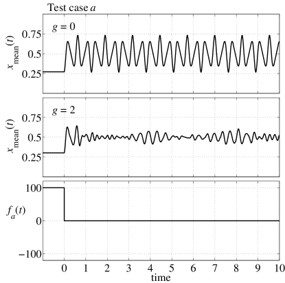
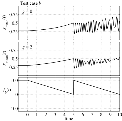
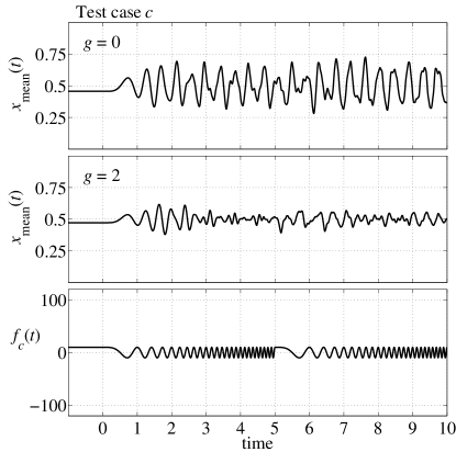
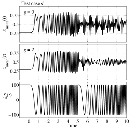
Figure 1: Dynamics of the test systems The mean position $x_{\mathrm{mean}}(t)$ of the $N=5$ particles in the well; see details in the text. To see how the interactions between particles affect the result, both the cases $g=0$ and $g=2$ are included. The function $f(t)$ that determines the strength of the tilted bottom is also plotted for each case.

3.2 Test results and discussion

The various methods discussed in section 2 were tested and compared, for the test case discussed above. To summarize, the exponential integrator based methods (ALC, AL1 and AL2) were found to perform well, in particular for large basis sizes, and when the Hamiltonian itself is not changing too strongly and rapidly in time. Details are given below.

3.2.1 Performance measurement

With large dimensions of the Hilbert space, most of the computational time required is used to form matrix-vector products between the Hamiltonian and some vector. For all the methods considered here, all other calculations involved can be expected to take much less time, typically being scalar products or additions of vectors. Performance is therefore here measured in the number of such matrix-vector multiplications that a method needs in order to produce $|\Psi(t=10)\rangle$.

3.2.2 Numerical parameters

Some remarks should be made regarding the various numerical tolerances for the different methods. The aim in this study was to find methods which are accurate enough, so that the global error should be smaller than $10^{-2}$ (that is, for the present test case, $\||\Psi_{\mathrm{approx}.}(t=10)\rangle-|\Psi_{\mathrm{correct}}(t=10)\rangle\|_{2}<10^{-2}$). This was here assumed to be fulfilled if the solutions obtained with different methods did not differ by more than $10^{-2}$. An error of this order implies that expectation values of the calculated states should be accurate enough, so that one can draw qualitative conclusions about the underlying physics.

After extensive testing, all error tolerances used for the methods ALC, AL1, AL2 and RK8 were eventually fixed to $10^{-6}$. The various tolerances essentially control the local error per time step, so that it seems reasonable that the appropriate values should be similar for the different methods. In any case, larger values occasionally gave too large global errors, and the aim here was to find robust methods needing as little tuning as possible.

Regarding the parameter $d_{1}$, the number of single-particle orbitals used in the basis, an increased $d_{1}$ gives a higher spatial accuracy. For the present test case, the resulting $x_{\mathrm{mean}}(t)$ change a bit when $d_{1}$ is increased from $10$ to $20$, but the difference when increasing $d_{1}$ to $30$ is barely visible on the scale of Fig. 1. A stronger tilted potential, or a stronger interaction between the particles, would require more orbitals to be used in order to achieve accurate results. A larger dimension $d_{1}=40$ is also included in Table 1, but because of practical time limitations only the method AL1 was tested for that case.

3.2.3 Test results

Test results for the methods presented in section 2, are given in Table 1, for various choices of basis sizes and time-dependent potentials. For the different cases, the number of matrix-multiplications required by a method to produce $|\Psi(t=10)\rangle$ are given in the respective columns. With the numerical parameters set as discussed above, the error between solutions obtained with different methods were typically of the order $10^{-3}$.

For case (a) with a constant Hamiltonian, the ALC method was substantially more efficient than any of the other methods, needing fewer matrix-vector multiplications. As one might expect from their differences with ALC, the methods AL1 and AL2 need to do more work to control the error – essentially they to compute each time step twice. In this sense there is no point in actually using those methods for constant Hamiltonians, but the present test results imply that the adaptivity works fairly well, given how they operate.

Generally, AL1 was more efficient than AL2. Regarding the Runge-Kutta method (RK8), it appears to be indifferent to the time-dependence in the Hamiltonian, such that it does about the same amount of work for each of the four cases. Contrary to this, AL1 and AL2 have to work harder when the time-dependence becomes more influential, as in case d, although they are still more efficient than RK8 for the largest basis sizes.

For all the methods, except ALC, it will occasionally happen that a time step needs to be re-done with a smaller $\Delta t$ in order to keep the error small enough. Thus, some matrix-vector multiplications will have been wasted. These are included in the values reported in Table 1, but typically constituted only a few percent of the total count.

Several other choices of basis sizes, particle numbers and time-dependent potentials were tested as well, apart from those reported in Table 1, and all were found to give consistent results.

$f(t)$	$d_{1}$	$d_{N}$	ALC	AL1	AL2	RK8
a	10	2002	16200	36040	50622	87229
	20	42504	74670	128850	182466	347172
	30	278256	160050	297104	355938	780333
	40	1086008	–	568560	–	–
b	10	2002	–	64623	81176	92452
	20	42504	–	148960	165565	352094
	30	278256	–	302143	290137	785391
	40	1086008	–	559624	–	–
c	10	2002	–	108039	132063	87215
	20	42504	–	196115	232306	347160
	30	278256	–	320254	344869	780372
	40	1086008	–	558616	–	–
d	10	2002	–	301651	357154	105479
	20	42504	–	326627	410428	347267
	30	278256	–	459331	609458	780854
	40	1086008	–	653302	–	–

Table 1: Test results The number of matrix-vector multiplications required by a method to produce $|\Psi(t=10)\rangle$ are listed for the four different methods denoted by ALC, AL1, AL2 and RK8 (see section 2). Tests were run for different time-dependent potentials modulated by different functions $f(t)$ (cases a, b, c and d, see section 3.1.1), and using different numbers $d_{1}$ of basis orbitals (see section 3.1.2). For the $N=5$ particles in the system, the resulting Hilbert space dimension is $d_{N}$ (that is, the matrix has dimensions $d_{N}\times d_{N}$). Since the ALC method is only applicable for constant Hamiltonians, some cells are empty. Also, because of practical time limitations, only the AL1 method was tested for the case $d_{1}=40$. As discussed in section 3.2.2, already $d_{1}=30$ gave sufficient spatial accuracy. The error between solutions produced by different methods was typically of the order $10^{-3}$, and never larger than $10^{-2}$.

3.2.4 Comparison with other methods

A number of other methods were also tested. A commonly used 5:th order Runge-Kutta method, also designed by Dormand and Prince [46], was found to require about 70% more matrix-vector multiplications than the 8:th order version (see section 2.3), for the present test case. In Ref. [46] three variants are given of the 5:th order method; in this study the one called RK5(4)7M was found to be the most efficient of those, in agreement with what the authors concluded.

In order to compare with existing widely used implementations, some of the routines in the commercial software package Matlab [45] were also tested. As one should expect, that implementation of the 5:th order Dormand-Prince method (called ode45 [47]) had almost identical performance to the one made in this study. Another Matlab routine, called ode23 [47], using a lower-order Runge-Kutta method, was found to be less efficient. The Matlab routine ode113 [47], using a multi-step Adams-Bashforth-Moulton method, was found to be almost as efficient as the 8:th order Runge-Kutta method discussed above (RK8). A relevant question is if any of the Matlab routines intended for stiff problems would be more suitable, but this seems unlikely from the results discussed in section A.2, where the implicit Crank-Nicolson method is tested.

3.2.5 Discussion

For a constant Hamiltonian, the ALC method, originally presented by Park and Light [10], clearly appears to be the best choice, from the results in Table 1.

When the Hamiltonian explicitly depends on time, the AL1 method was generally found to be the most efficient. If, somehow, the two different steps used in the AL2 method could somehow be embedded in each other, similar to embedded Runge-Kutta formulas [39], then AL2 would perform better than AL1, as the numbers of multiplications it needs could then be reduced by one third. However, despite various schemes attempted during the course of this study, no practical way was found.

As discussed, the time step $\Delta t$ used by the AL1 and AL2 methods was determined adaptively. Perhaps counter-intuitively, it was of the same order throughout the entire evolution with the sawtooth function (case b), even though the particles in the system have very different dynamics in different time intervals, as shown in Fig. 1. In other words, the numerical work required was about the same whether the evolution was adiabatic or not.

Another relevant issue to keep in mind is the actual development work needed to implement the methods. From this perspective, the RK8 method is very easy to work with, at least relative to the others. Apart from the matrix-vector multiplications, it only requires regular vector operations like addition and scaling. It does not rely on more sophisticated numerical algorithms, such as eigenvalue determination. And it is fairly straightforward to implement following the self-contained presentation in, for example, the original Ref. [42].

4 Summary

In this study, various numerical methods for solving the time-dependent Schrödinger equation have been compared, for few-body systems with strong interactions between the particles, and with an explicitly time-dependent Hamiltonian. Using the configuration interaction method, one obtains a linear system of ordinary differential equations, which in principle is a standard problem. However, the typically very large dimensions make it important to find optimal methods.

In agreement with what has been stated by other authors (see for example Ref. [14]), so called exponential integrator methods were found to perform better than other methods designed for more general differential equations. For the case of a time-independent Hamiltonian, a method described in Ref. [10] was found to perform very well (denoted ALC above), but it is not applicable when the Hamiltonian has an explicit time-dependence. In this case, two extended algorithms were suggested here, which implement adaptivity in a different way. They were found to be more efficient than all other methods tested here.

Both the extended algorithms compute each time step twice, to obtain two solutions where one is known to be more accurate than the other. In short, if the difference between the solutions is small enough, the simulation can continue, otherwise the time step is re-done with a smaller step size. In one of the approaches the second order Magnus approximation was used and compared with the first order variant – this provided two solutions that could be compared (this method is denoted AL2 above). While this scheme worked well, an alternative implementation was found to be even more efficient; using only the first order approximation combined with step-doubling to obtain the more accurate solution (the approach denoted AL1 above). Regarding other types of methods, the most efficient of those that were tested here was an 8:th order Runge-Kutta formula, with an embedded 7:th order formula to provide the two solutions (RK8) [42]. While being less efficient than the exponential-integrator based methods, it is, relative to the other methods, easier to implement. An implicit method was also tested, as discussed in the appendix, but found to be inefficient.

Certainly, further development and refinement may improve the performance of the methods AL1 and AL2. One interesting point to address is if the local error estimate can be computed in a more efficient way, to avoid the double time evolutions, perhaps similar in fashion to embedded Runge-Kutta formulas. Another issue is the various numerical parameters involved; their interplay is not obvious, and more careful tuning may improve the performance. In any case, though, the perhaps naive choices made in this study easily resulted in methods which performed very well.

Appendix A Appendix

A.1 Remarks about the implementation

A.1.1 Restrictions on the Hamiltonian

While the aim here was to find methods for as general Hamiltonians as possible, one restriction was applied. The implementation made in this study only handles time-dependent Hamiltonians that can be written on the form

$$H(t)=A+f(t)B$$ (12)

such that the matrices $A$ and $B$ are constant throughout the time evolution, and the entire time dependence is contained in the scalar function $f(t)$. This form still allows one to simulate a number of relevant physical systems, such as electrons in a laser field, or ultra-cold atoms with time-dependent interactions governed by an external field. No assumption is made about the relative magnitudes of the two matrices, or whether they are for example one- or two-body operators. In principle, both matrices could have time-dependent prefactors, and there could be additional similar terms. The important thing is to be able to form the product between the matrix $\Omega_{1}$ or $\Omega_{2}$ with an arbitrary vector (see Eqs. (8) and (10)), at any time $t$, and for any $\Delta t$. With the restriction in Eq. (12) above, and with Simpson’s rule to approximate the integrals, these matrices reduce to

$$\Omega_{1}(t,\Delta t)\approx-i\Delta tA-i\frac{\Delta t}{6}\biggl{(}f(t)+4f(t+\frac{\Delta t}{2})+f(t+\Delta t)\biggl{)}B$$ (13)

and

$$\Omega_{2}(t,\Delta t)\approx\frac{(\Delta t)^{2}}{12}\biggl{(}f(t+\Delta t)-f(t)\biggl{)}[A,B]$$ (14)

so that one only needs to form the multiplication of $A$ or $B$ with arbitrary vectors, and then scale the products.

A.1.2 Breakdown of the Lanczos process

In the Lanczos process, when a Krylov space and the associated tridiagonal matrix is generated – see Eq. (4) – it may happen that some $\beta$-value is zero. This implies that a subspace has been found from which the state $|\Psi(t)\rangle$ cannot escape, which is fortunate since it makes the time evolution easier. A typical example would be if the Hamiltonian does not change in time, and the initial state happens to be an eigenstate. While such a breakdown does not cause any fundamental problem for the time evolution, it needs to be handled in an implementation.

A.1.3 Initial guess for $\Delta t$

Given some time interval $[t_{\mathrm{begin}},t_{\mathrm{end}}]$ during which the time evolution is to be calculated, some initial guess for the time step $\Delta t$ is needed in the methods. In the present implementation this was made by simply starting with $\Delta t=t_{\mathrm{end}}-t_{\mathrm{begin}}$, and then let the methods adjust it themselves, as described in section 2.

A.2 An implicit method

Typically, the eigenvalues of the Hamiltonian matrix may be very different in magnitude, because of the different energies of the basis states used. This implies that the problem may be stiff, so that an implicit solver might be more efficient than an explicit one [39]. In an initial phase of this study, the Crank-Nicolson (CN) method [48] was tested. It is an implicit method similar to the Euler backward method, such that it is stable, but of higher accuracy. Given the state $|\Psi(t_{0})\rangle$, the next state $|\Psi(t_{0}+\Delta t)\rangle$ is defined implicitely by the equation

$$\biggl{(}1+i\frac{\Delta t}{2}H(t_{0}+\Delta t)\biggl{)}|\Psi(t_{0}+\Delta t)\rangle=\biggl{(}1-i\frac{\Delta t}{2}H(t_{0})\biggl{)}|\Psi(t_{0})\rangle$$ (15)

To obtain the state $|\Psi(t_{0}+\Delta t)\rangle$, one here needs to solve a system of linear equations. For this purpose, the generalized minimum residual method (GMRES) [25, 49, 50] was used here. It is an iterative method which, given an initial guess, converges towards the solution by use of repeated matrix-vector multiplications, making it suitable to use with large and sparse matrices. For the present application the method typically converged within 5–10 iterations (here, this was when the residual was less than $10^{-6}$). The Euler forward method was used to generate the initial guess.

However, it appears that the physical problem studied here was not sufficiently stiff to make an implicit method competitive. Or, perhaps, that so high accuracy is required that a higher-order method is needed (as also discussed in Ref. [14] for this class of problems). Table 2 shows some results from a comparison with the (explicit) classical fourth-order Runge-Kutta method [39], for the test case above with $N=2$ particles. As discussed in section 3.2, performance is here measured in the number of matrix-vector multiplications needed. For this test, the methods were not implemented to be adaptive, and instead a manually chosen fixed time step $\Delta t$ was used throughout the simulation. The obtained solution was then compared with that produced by the adaptive Lanczos solver described above for constant Hamiltonians (ALC). The time step was adjusted to give an error less than $0.01$, and to limit the available parameter space only time steps defined by two significant digits were considered (for example $\Delta t=0.014$ or $0.015$, but not $0.0145$). As shown in Table 2, the Crank-Nicolson method required considerably more multiplications than the explicit method.

		RK4		CN
$d_{1}$	$d_{N}$	mults.	$\Delta t_{\mathrm{RK4}}$	mults.	$\Delta t_{\mathrm{CN}}$
20	210	56340	0.00071	285797	0.00014
40	820	235296	0.00017	800003	0.000050

Table 2: Test results for the explicit fourth-order Runge Kutta method (RK4) and the implicit Crank-Nicolson (CN); see details in the text, and see also the explanation of captions in Table 1. The constant Hamiltonian from test case a was considered here, with $N=2$ particles. The CN method requires considerably more multiplications than the RK4 method. When comparing with the results in Table 1, it should be noted that the numbers here do not include any cost for adaptivity, as the fixed time step $\Delta t$ was adjusted manually. The error is here defined as $\|\Psi_{\mathrm{RK4/CN}}-\Psi_{\mathrm{ALC}}\|_{2}$, the difference with the solution obtained using the ALC method. Several other choices of basis sizes, particle numbers and time-dependent potentials were tested, and all were found to give very similar results, also for much larger problem dimensions.

Acknowledgements

This work was supported by the Swedish Research Council and the Nanometer Structure Consortium at Lund University.

References

- [1] C. E. Wieman, D. E. Pritchard, D. J. Wineland, Atom cooling, trapping, and quantum manipulation, Reviews of Modern Physics 71, S253 (1999)
- [2] F. Dalfovo, S. Giorgini, L. P. Pitaevskii, S. Stringari, Theory of Bose-Einstein condensation in trapped gases, Reviews of Modern Physics 71, 463 (1999)
- [3] I. Bloch, Ultracold quantum gases in optical lattices, Nature Physics 1, 23 (2005)
- [4] I. Bloch, J. Dalibard, W. Zwerger, Many-body physics with ultracold gases, Reviews of Modern Physics 80, 88 (2008)
- [5] S. Giorgini, L. P. Pitaevskii, S. Stringari, Theory of ultracold atomic Fermi gases, Reviews of Modern Physics 80, 1215 (2008)
- [6] F. Serwane, G. Zürn, T. Lompe, T. B. Ottenstein, A. N. Wenz, S. Jochim, Deterministic preparation of a tunable few-fermion system, Science 332, 336 (2011)
- [7] S. M. Reimann, M. Manninen, Electronic structure of quantum dots, Reviews of Modern Physics 74, 1283 (2002)
- [8] L. Samuelson, M. T. Björk, K. Deppert, M. Larsson, B. J. Ohlsson, N. Panev, A. I. Persson, N. Sköld, C. Thelander, L. R. Wallenberg, Semiconductor nanowires for novel one-dimensional devices, Physica E 21, 560 (2004)
- [9] R. Hanson, L. P. Kouwenhoven, J. R. Petta, S. Tarucha, L. M. K. Vandersypen, Spins in few-electron quantum dots, Reviews of Modern Physics 79, 1217 (2007)
- [10] T. J. Park and J. C. Light, Unitary time evolution by iterative Lanczos reduction, J. Chem. Phys. 85, 5870 (1986)
- [11] C. J. Cramer, Essentials of Computational Chemistry – Theories and Models (2nd Ed.), John Wiley & Sons, ISBN 0-470-09181-9 (2004)
- [12] P. Navrátil, S. Quaglioni, I. Stetcu, B. R. Barrett, Recent developments in no-core shell-model calculations, Journal of Physics G: Nuclear and Particle Physics 36, 083101 (2009)
- [13] M. Rontani, C. Cavazzoni, D. Belluci, and G. Goldoni, Full configuration interaction approach to the few-electron problem in artificial atoms, J. Chem. Phys. 124, 124102 (2006)
- [14] M. Hochbruck and A. Ostermann, Exponential integrators, Acta Numer. 19, 209 (2010)
- [15] T. Klamroth, Laser-driven electron transfer through metal-insulator-metal contacts: Time-dependent configuration interaction singles calculations for a jellium model, Phys. Rev. B 68, 245421 (2003)
- [16] R. E. Larsen and B. J. Schwartz, Efficient real-space configuration-interaction method for the simulation of multielectron mixed quantum and classical nonadiabatic molecular dynamics in the condensed phase, J. Chem. Phys. 119, 7672 (2003)
- [17] P. Krause, T. Klamroth, and P. Saalfrank, Time-dependent configuration-interaction calculations of laser-pulse-driven many-electron dynamics: Controlled dipole switching in lithium cyanide, J. Chem. Phys. 123, 074105 (2005)
- [18] N. Rohringer, A. Gordon, and R. Santra, Configuration-interaction-based time-dependent orbital approach for ab initio treatmen of electronic dynamics in a strong optical laser field, Phys. Rev. A 74, 043420 (2006)
- [19] P. Krause, T. Klamroth, and P. Saalfrank, Molecular response properties from explicitly time-dependent configuration interaction methods, J. Chem. Phys. 127, 034107 (2007)
- [20] S. Pabst, L. Greenman, P. J. Ho, D. A. Mazziotti, and R. Santra, Decoherence in attosecond photoionization, Phys. Rev. Lett. 106, 053003 (2011)
- [21] D. Hochstuhl and M. Bonitz, Time-dependent restricted active space configuration interaction for the photoionization of many-electron atoms, arXiv:1207.5693
- [22] A. I. Streltsov, O. E. Alon, and L. S. Cederbaum, Role of excited states in the splitting of a trapped interacting Bose-Einstein condensate by a time-dependent barrier, Phys. Rev. Lett. 99, 030402 (2007)
- [23] O. E. Alon, A. I. Streltsov, and L. S. Cederbaum, Multiconfigurational time-dependent Hartree method for bosons: Many-body dynamics of bosonic systems, Phys. Rev. A 77, 033613 (2008)
- [24] C. Lanczos, An iteration method for the solution of the eigenvalue problem of linear differential and integral operators, J. Res. Nat. Bur. Stand. 45, 255 (1950)
- [25] G. H. Golub and C. F. van Loan, Matrix Computations, 3rd Ed., ISBN 0-8018-5414-8, John Hopkins University Press (1996)
- [26] Y. Saad, Analysis of some Krylov subspace approximations to the matrix exponential operator, SIAM J. Numer. Anal. 29, 209 (1992)
- [27] M. Hochbruck and C. Lubich, On Krylov subspace approximations to the matrix exponential operator, SIAM J. Numer. Anal. 34, 1911 (1997)
- [28] M. Hochbruck, C. Lubich, and H. Selhofer, Exponential integrators for large systems of differential equations, SIAM J. Sci. Comput. 19, 1552 (1998)
- [29] M. Hochbruck and C. Lubich, Exponential integrators for quantum-classical molecular dynamics, BIT 39, 620 (1999)
- [30] W. S. Edwards, L. S. Tuckerman, R. A. Friesner, and D. C. Sorensen, Krylov methods for the incompressible Navier-Stokes equations, J. Comp. Phys. 110, 82 (1994)
- [31] R. B. Sidje, Expokit: A software package for computing matrix exponentials, ACM Trans. Math. Soft. 24, 130 (1998)
- [32] L. Bergamaschi, M. Caliari, A. Martìnez, and M. Vianello, Comparing Leja and Krylov approximations of large scale matrix exponentials, Computational Science – ICCS, Lecture Notes in Computer Science 3994, 685 (2006)
- [33] W. Magnus, On the exponential solution of differential equations for a linear operator, Comm. Pure Appl. Math. 7, 649 (1954)
- [34] R. M. Wilcox, Exponential operators and parameter differentiation in quantum physics, J. Math. Phys. 8, 962 (1967)
- [35] F. Fer, Résolution de l’équation matricielle par produit infini d’exponentielles matricielles, Bull. Classe Sci. Acad. R. Belg. 44, 818 (1958)
- [36] S. Klarsfeld and J. A. Oteo, Exponential infinite-product representations of the time-displacement operator, J. Phys. A: Math. Gen. 22, 2687 (1989)
- [37] R. Kosloff, Propagation methods for quantum molecular dynamics, Annu. Rev. Phys. Chem. 45, 145 (1994)
- [38] M. Hochbruck and C. Lubich, On Magnus integrators for time-dependent Schrödinger equations, SIAM J. Numer. Anal. 41, 945 (2003)
- [39] W. H. Press, S. A. Teukolsky, W. T. Vetterling, B. P. Flannery, Numerical recipes in C: The art of scientific computing, 2nd Ed., ISBN 0-521-43108-5, Cambridge University Press (1992)
- [40] D. J. Tannor, A. Besprozvannaya, and C. J. Williams, Nested interaction representations in time dependent quantum mechanics, J. Chem. Phys. 96, 2998 (1992)
- [41] K. Kormann, S. Holmgren, and H. O. Karlsson, Accurate time propagation for the Schrödinger equation with an explicitly time-dependent Hamiltonian, J. Chem. Phys. 128, 184101 (2008)
- [42] P. J. Prince and J. R. Dormand, High order embedded Runge-Kutta formulae, Journal of Computational and Applied Mathematics 7, 67 (1980)
- [43] M. Girardeau, Relationship between systems of impenetrable bosons and fermions in one dimension, J. Math. Phys. 1, 516 (1960)
- [44] M. Born and V. Fock, Beweis des Adiabatensatzes, Z. Phys. 51, 165 (1928)
- [45] MATLAB 7.10.0 (R2010a), The MathWorks, Inc., Natick, Massachusetts, United States
- [46] J. R. Dormand and P. J. Prince, A family of embedded Runge-Kutta formulae, Journal of Computational and Applied Mathematics 6, 1 (1980)
- [47] L. F. Shampine and M. W. Reichelt, The Matlab ODE suite, SIAM J. Sci. Comput. 18, 1 (1997)
- [48] J. Crank and P. Nicolson, A practical method for numerical evaluation of solutions of partial differential equations of the heat conduction type, Proc. Camb. Phil. Soc. 43, 50 (1947)
- [49] Y. Saad and M. H. Schultz, GMRES: A generalized minimal residual algorithm for solving nonsymmetric linear systems, SIAM J. Sci. Stat. Comput. 7, 856 (1986)
- [50] R. Barrett, M. Berry, T. F. Chan, J. Demmel, J. M. Donato, J. Dongarra, V. Eijkhout, R. Pozo, C. Romine, H. van der Vorst, Templates for the Solution of Linear Systems: Building Blocks for Iterative Methods, 2nd Ed., SIAM, Philadelphia, PA (1994)