Fast non parametric entropy estimation for spatial-temporal saliency method

Abstract

This paper formulates bottom-up visual saliency as center surround conditional entropy and presents a fast and efficient technique for the computation of such a saliency map. It is shown that the new saliency formulation is consistent with self-information based saliency, decision-theoretic saliency and Bayesian definition of surprises but also faces the same significant computational challenge of estimating probability density in very high dimensional spaces with limited samples. We have developed a fast and efficient nonparametric method to make the practical implementation of these types of saliency maps possible. By aligning pixels from the center and surround regions and treating their location coordinates as random variables, we use a k-d partitioning method to efficiently estimating the center surround conditional entropy. We present experimental results on two publicly available eye tracking still image databases and show that the new technique is competitive with state of the art bottom-up saliency computational methods. We have also extended the technique to compute spatiotemporal visual saliency of video and evaluate the bottom-up spatiotemporal saliency against eye tracking data on a video taken onboard a moving vehicle with the driver’s eye being tracked by a head mounted eye-tracker.

1 Introduction

In recent years, there has been increasing interest in the application of the visual saliency mechanism to computer vision problems. A predominant theory of the computational visual saliency models is the ”center-surround” mechanism that is ubiquitously found in the early stages of biological vision HUBEL1965 . In the literature, a number of computational models that are in one way or another based on such center-surround theory have been proposed. Arguably one of the most popular models is that of Itti and Koch itti1998model which computes saliency of a location based on the difference of the low-level features between the center and its surrounds. Many variants of this model that directly compute the low-level center surround differences have subsequently appeared in the literature including those perform the computation in the frequency domain such as Hou2007 and Guo2008 . An approach that is based on information theory and captures the center surround differences through self-information of a location in the context of a given image or a group of other images has been proposed by Bruce and Tsotos Bruce2006b . Another model that is based on decision theory has been proposed by Gao et al.Gao2007 which computes the saliency of a location through the mutual information between the low- and intermediate-level features of the location and its surrounds. From a computational perspective, Gao2007 and Bruce2006b share some similarities in the sense that whilst Bruce2006b computes self-information Gao2007 computes mutual information. Another approach that takes a radically different strategy is that of Judd et al.Judd2009 who proposed a learning from example ideas to compute visual saliency.

A major difficulty with models that are based on the computation of information quantities such as self-information Bruce2006b and mutual information such as Gao2007 is that they are computationally challenging - involving estimating probability density functions in very high dimensional spaces with limited samples. The authors of Bruce2006b used independent component analysis (ICA) to project high dimensional image patches onto independent subspace such that the self-information can be estimated through 1-d histograms of the independent components. Computing the data dependent ICA bases is in itself computational expensive, although some authors have shown that ICA can be replaced by data independent transforms such as discrete cosine transform Qiu2007 , computing the transform itself is also computationally demanding. The authors of Gao2007 got around the computational difficulty of estimating the mutual information by using a parametric Generalized Gaussian Distribution (GGD) to approximate the probability densities of band-pass center and surround features. To do this, they had to resort to statistics of various features of natural images to estimate the parameters of the GGD’s. However, there exists some uncertainties about the model, and even the authors acknowledged ambivalence with respect to the importance of the shape parameter Gao2007 .

In this paper, we follow the center surround principle of visual saliency and directly formulate the bottom-up saliency of a location as the conditional entropy of the center given its surround. As the conditional entropy measures the remaining entropy (or uncertainty, informativeness, or surprise) of the center after observing the surrounds, this formulation is related to previous saliency models of self-information Bruce2006b , mutual information Gao2007 and Bayesian surprise Itti2006 . The center surround conditional entropy formulation gives a direct and intuitive interpretation of the center surround mechanism and also facilitates the easy extension to spatio-temporal saliency. As with related models, a significant challenge is the estimation of probability density functions in high dimensional spaces with limited samples. A major contribution of this paper is the development of a fast and practical solution based on non-parametric multidimensional k-d tree entropy estimation Stowell2009a to make such kinds of approaches computationally tractable and make them applicable in real-time applications such as saliency detection in videos. We present experimental results on several publicly available eye-tracking still image databases Bruce2006b ; Judd2009 and a video taken on-board a car with the driver’s eye movement being tracked with a head-mounted eye tracker to demonstrate the effectiveness of the proposed method and compare it with existing techniques.

2 Saliency based on Center-Surround Conditional Entropy and Kullback-Leibler Divergence

Let $I_{c}(\emph{x},\emph{y})$ be an image patch at location $(\emph{x},\emph{y})$ and $I_{sr}(\emph{x},\emph{y})$ its surrounding regions. The conditional entropy of the center given its surround can be defined as

$$\emph{{H}}(I_{c}(\emph{x},\emph{y})|I_{sr}(\emph{x},\emph{y}))=\emph{{H}}(I_{c}(\emph{x},\emph{y}),I_{sr}(\emph{x},\emph{y}))-\emph{{H}}(I_{sr}(\emph{x},\emph{y}))$$ (1)

and can be further defined in terms of joint and marginal probabilities

$$\emph{{H}}(I_{c}(\emph{x},\emph{y})|I_{sr}(\emph{x},\emph{y}))=\sum_{\begin{subarray}{c}I_{c}(\emph{x},\emph{y})\in\emph{{I}}\\ I_{sr}(\emph{x},\emph{y})\in\emph{{I}}\end{subarray}}p(I_{c}(\emph{x},\emph{y}),I_{sr}(\emph{x},\emph{y}))log\frac{p(I_{sr}(\emph{x},\emph{y}))}{p(I_{c}(\emph{x},\emph{y}),I_{sr}(\emph{x},\emph{y}))}$$ (2)

The conditional entropy $\emph{{H}}(I_{c}(\emph{x},\emph{y})|I_{sr}(\emph{x},\emph{y}))$ can be understood in a number of ways. From a coding or information theory’s perspective, it will take $\emph{{H}}(I_{c}(\emph{x},\emph{y}),I_{sr}(\emph{x},\emph{y}))$ bits to code the center and its surrounds together, but if we knew the surround $I_{sr}(\emph{x},\emph{y})$ already, we will have gained $\emph{{H}}(I_{sr}(\emph{x},\emph{y}))$ bits of information, and the conditional entropy measures the remaining bits needed to code the center. From an uncertainty or informativeness point of view, the conditional entropy measures the remaining uncertainty of the center once its surrounds are known, or the amount of information of the center given the knowledge of its surrounds. We can use the conditional entropy or Kullback-Leibler divergence as a measure of saliency, i.e.

$$\emph{{S}}(\emph{x},\emph{y})=\emph{{H}}(I_{c}(\emph{x},\emph{y})|I_{sr}(\emph{x},\emph{y}))\text{ or }\emph{{S}}(\emph{x},\emph{y})=\emph{{D}}(I_{c}(\emph{x},\emph{y})|I_{sr}(\emph{x},\emph{y}))$$ (3)

The definition of saliency in equation (3) and (2) is consistent with a number of definitions in the literature including self-information Bruce2006b , surprise Itti2006 and decision theoretic saliency Gao2007 . The self-information saliency of Bruce2006b measures the self-information of $I_{c}(\emph{x},\emph{y})$ in the context of its surrounds, $-log\{p(I_{c}(\emph{x},\emph{y}))\}$. If $I_{c}(\emph{x},\emph{y})$ is a common patch within the image, then $p(I_{c}(\emph{x},\emph{y}))$ is large, $-log\{p(I_{c}(\emph{x},\emph{y}))\}$ will be small, hence the saliency will be small. $\emph{{S}}(\emph{x},\emph{y})$ in (3) has the same property, that is, if the center and its surrounds are very similar, then $\emph{{S}}(\emph{x},\emph{y})$ will be small and conversely, if they are very different, it will be large. The surprise measure of Itti2006 can be re-written as

$$\emph{{S}}=\sum_{\begin{subarray}{c}I_{c}(\emph{x},\emph{y})\in\emph{{I}}\\ I_{sr}(\emph{x},\emph{y})\in\emph{{I}}\end{subarray}}p(I_{sr}(\emph{x},\emph{y}))log\frac{p(I_{sr}(\emph{x},\emph{y}))}{p(I_{sr}(\emph{x},\emph{y})|I_{c}(\emph{x},\emph{y}))}$$ (4)

Here, the surrounds $I_{sr}(\emph{x},\emph{y}))$ can be interpreted as the model or background information and the center $I_{c}(\emph{x},\emph{y})$ as the new observation data. Comparing to our formulated definition of center-surround entropy in terms of Kullback-Leibler divergence,

$$\emph{{D}}(I_{c}(\emph{x},\emph{y})|I_{sr}(\emph{x},\emph{y}))=\sum_{\begin{subarray}{c}I_{c}(\emph{x},\emph{y})\in\emph{{I}}\\ I_{sr}(\emph{x},\emph{y})\in\emph{{I}}\end{subarray}}p(I_{c}(\emph{x},\emph{y}))log\frac{p(I_{sr}(\emph{x},\emph{y}))}{p(I_{c}(\emph{x},\emph{y}))}$$ (5)

There is a great similarity between two types of saliency measurements defined by equations 5 and 4, so are their responses to input data. Again, the surprise measure will be small when the center and surround are similar and large when they are different. The decision theoretic discriminant saliency of Gao2007 boils down to the computation of the mutual information between the center and its surround, and the mutual information and the conditional entropy has the following relation.

$$\emph{{MI}}(I_{c}(\emph{x},\emph{y}),I_{sr}(\emph{x},\emph{y}))=\emph{{H}}(I_{c}(\emph{x},\emph{y}))-\emph{{H}}(I_{c}(\emph{x},\emph{y})|I_{sr}(\emph{x},\emph{y}))$$ (6)

$\emph{{MI}}(I_{c}(\emph{x},\emph{y}),I_{sr}(\emph{x},\emph{y}))$ is the amount of uncertainty of the center $I_{c}(\emph{x},\emph{y})$ that is removed when its surrounds $I_{sr}(\emph{x},\emph{y})$ are known. One way to understand MI is that it measures how much the surround can tell about the center which is again consistent with the conditional entropy. A large mutual information means the surround can tell a lot about the center hence the saliency will be low, so will be the center surround conditional entropy.

For all these definitions of saliency measure, there is a fundamental challenge - practical implementation. As all involve the estimation of probability density functions in very high dimensional spaces with limited data samples, various simplification processes have to be used, e.g., Bruce2006b employed independent component analysis and Gao2007 assumed a parametric GGD model. In the next section, we introduce a fast non-parametric method.

3 Fast Estimation of Conditional Entropy based Saliency and Kullback-Leibler Divergence

Visual data have excessive amount of information, but only some of them is useful for forming saliency maps. Itti et al.itti1998model used low-level features of intensity, colour and orientation to build several conspicuity maps which are combined in a linear fashion to generate a saliency map. In the discriminant saliency map approach, Gao et al.Gao2007 used wavelet and Gabor filters to extract band-pass features and modeled these features using parametric Generalized Gaussian distribution (GGD) to estimate the mutual information between the center and surround. In this paper, we use medium frequencies features since studies have shown showed that mid-band frequency data globally allow the best prediction of attention for many categories of scenes Urban2010 .

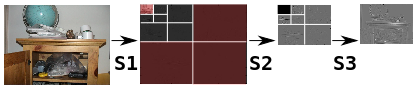
Figure 1: Medium Band Filter Flow Chart

Figure 1 shows a step-by-step illustration of mid-band filtering used in this paper. In the first step, a 9/7 Cohen-Daubechies-Feauveau (CDF) waveletCohen1992 is used to analyse the image into three different frequency bands. After isolating different frequency bands of the visual data, the DC parts and highest frequency-band components, level 3, are removed in step 2. The remaining components are converted back to the image domain by the inverse of the 9/7 CDF wavelet in step 3. DC component is filtered out in order to remove global trend of signals or images while the proposed saliency method mainly depends on center-surround mechanism or local difference between central and surround patches. Removals of wavelet coefficients level 1 is mainly due to noise reduction purpose. These two steps named as Medium Subband Filter (MSF) is proved to be biologically plausible; Urban et al.Urban2010 carries out several experiments on correlation between eye fixation data and image features of different frequency bands and concluded that human visual performance well coordinates with image features from wavelet frequency band L2 to L4. More details can be found from Urban paper Urban2010 . In addition to that good relativity between psychological data and MSF features, another advantage of MSF is cleaning data since it removes DC global trend and noise signals to which the proposed entropy estimation method is very sensible. 5.

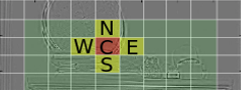
Figure 2: Effective Saliency Region

After medium frequency filtering, the outputs of the step 3 are divided in 8x8 patches as shown in Figure 2. Although other patch sizes are possible, 8x8 patches were used in this paper. From those filtered data in patches, saliency values can be estimated as conditional entropy of central data given surrounding data or statistical Kullback-Leibler divergence of data between center and surround patch 3

First, we consider the saliency as the conditional entropy of each center patch (C) given its four surrounding patches (N, S, W, and E) as shown in Figure 2. The conditional entropy based saliency is computed as

$$S(\textbf{C})=H(\textbf{C}|(\textbf{N},\textbf{S},\textbf{W},\textbf{E}))=H(\textbf{C},\textbf{N},\textbf{S},\textbf{W},\textbf{E})-H(\textbf{N},\textbf{S},\textbf{W},\textbf{E})$$ (7)

Estimating the two joint entropies on the right-hand side of (7) is challenging because of the high dimensionality of the data. To get round the problem, we take a similar approach as Viola1995 and treat the coordinate locations of the pixels as the random variables and approximate (7) as

$$S(\textbf{C})=H(c(\emph{x},\emph{y}),n(\emph{x},\emph{y}),s(\emph{x},\emph{y}),w(\emph{x},\emph{y}),e(\emph{x},\emph{y}))-H(n(\emph{x},\emph{y}),s(\emph{x},\emph{y}),w(\emph{x},\emph{y}),e(\emph{x},\emph{y}))$$ (8)

where $c(\emph{x},\emph{y}),n(\emph{x},\emph{y}),s(\emph{x},\emph{y}),w(\emph{x},\emph{y}),e(\emph{x},\emph{y})$ are respectively pixels from the $\textbf{C},\textbf{N},\textbf{S}$, $\textbf{W},\textbf{E}$ patches at the same reference location (x,y).

We treat the problem as drawing samples from (x,y) in order to approximate the conditional entropy. With the formulation of (8), we can now simplify the problem as estimating the entropies in the 4-D and 5-D spaces with a total of 8x8 = 64 samples.

We use a technique similar to Stowell2009a to achieve fast implementation of (8). The technique is based on a k-d tree style approach to partition the input data space $\Omega\in\Re^{D}$ into $\emph{A}=\{\emph{A}_{j}|\emph{j}=1,2,\ldots,\emph{m}\}$ with $\emph{A}_{i}\bigcap\emph{A}_{j}=\varnothing$ if $\emph{i}\neq\emph{j}$ and $\bigcup_{j}\emph{A}_{j}=\Omega$. Let $\emph{n}_{j}$ be the number of samples in the cell $\emph{A}_{j}$, $\emph{V}(\emph{A}_{j})$ the volume of cell $\emph{A}_{j}$, the total number of sample N, then the multidimensional joint entropy can be estimated as

$$\hat{H}=\sum_{j=1}^{m}\frac{n_{j}}{N}log\left(\frac{N}{n_{j}}V(A_{j})\right)$$ (9)

As well as conditional entropy, Kullback-Leibler divergence is another measure which suits into center-surround difference computation. According to the equation 5, the saliency of central patch is its divergence in accordance with the surrounding reference. Then, the computational task is figuring out $p(I_{sr}(\emph{x},\emph{y}))$ and $p(I_{c}(\emph{x},\emph{y}))$, where $I_{sr}(\emph{x},\emph{y})=\{n(x,y),s(x,y),e(x,y),w(x,y)\}$ and $I_{c}(\emph{x},\emph{y})=\{c(x,y)\}$ Once again, the technique proposed in Stowell2009a comes in handy. The k-d tree partition technique can be utilized to break data points into uniformly distributed cells where probability density function can be simply approximated with number of samples and its correspondent volumes. However, there is one distinguishing point between kdpee usage in conditional entropy and KL divergence estimation which is data ordering. In conditional entropy estimation $H(C|S)$, it does not matter that the joint entropy is computed as $H(C,S)$ or $H(S,C)$. However, that order has importance meaning in KL divergence which is asymmetric information measurement $D(C||S)<>D(S||C)$. Hence, before performing k-d partition, data should be organized such that first four dimensions contains data of surrounding patches, and the fifth dimension contains data of central patch. That data format causes surrounding data are partitioned before any central data is done. In other words, surrounding information already gives reference to the central partitioning tasks. The partition scheme ensures that number of samples in central cells and surrounding cells are equal $n^{sr}_{j}=n^{c}_{j}$, so the ratio $\frac{p(I_{sr}(x,y))}{p(I_{c}(x,y))}$ is equal to $\frac{V(A^{c}_{j})}{V(A^{s}_{j})}$. Therefore, the KL divergence $D(c(x,y)||{n(x,y),s(x,y),e(x,y),w(x,y)})$ in the equation 5 can be rewritten as.

$$\hat{D}=\sum_{j=1}^{m}\frac{n_{j}}{N}log\left(\frac{V_{c}(A_{j})}{V_{sr}(A_{j})}\right)$$ (10)

The computational complexity of either conditional entropy or KullbackLeibler approach is $\Theta\left(DNlogN\right)$ and the space complexity is $\Theta(DN)$. In our setting, $\emph{N}=64$ and $\emph{D}=5$ or $\emph{D}=4$. The lower limit of the sample size is $\emph{N}\geq 2^{D}$, $2^{5}=32$ and $2^{4}=16$, therefore our setting meets the samples size requirement of the algorithm.

Two measurements and approaches are nearly identical in their meanings, measurements of center-surround information, and computational methods, usage of kd tree partitioning. However, Kullback-Leibler divergence has quite a bit of advantages in computational expenses and preferred visual results. Both boil down to simple truths two kd partitioning jobs need to be done for conditional entropy measurement meanwhile KL divergence only requires once. Therefore, the later approach is essentially twice as fast as the former. In addition, KL divergence reduces the effect of bias in information estimation which are heavily affect saliency maps generated by difference between two entropy estimation. Therefore, it produces much smoother and eye-candy saliency maps.

Beside better performance, KL divergence possesses interesting theoretical points which help to measure bias in information estimation while conditional entropy does not clearly accounts for it. According to Gibbs’ inequality, Kullback-Leibler divergence must be positive; therefore, any negative KL divergence is a result of estimation bias. The bias is mainly due to samples shortage in high-dimensional data estimation; in other words, the bias ratio, number of biased estimation over the total number of estimation, depends on the size of patches, amount of available data for estimation. It paves a way for identifying data size which minimizes possible bias; for example, in 544x720 images, if the odd patch size, $n$, is varied between 7 and 21, we have bias correspondent bias ratio as follows.

Table 1: Bias ration vs. patch size

Patch size	7x7	9x9	11x11	13x13	15x15	17x17	19x19	21x21
Error ratio	0.0352	0.0250	0.0116	0.0046	0.0014	0.0002	0.0000	0.0000

Results in the table 1 points out that a size of patches may needs to reach 19 or 21 to totally eliminate bias in KL divergence estimation. Though 7x7 patch size is responsible for $3.52\%$ more bias estimation points than 21x21 patch size, it does not affect relative saliency value comparison between two points as long as they are estimated on the same number of data. Therefore, it does not causes any significant differences in normalized saliency maps. Choices of size patches does not cause much difference visually and numerically in normalized saliency maps, but it does affect performance in terms of speed. Obviously the more input data, the more processing time needs spending for processing them. In later experiments, 7x7 patches are mainly utilized, since it provides both reasonable saliency maps and computational efficiency.

4 Extension to Motion Video and Spatiotemporal Saliency

The techniques described in 2 and 3 can be easily extended to 3D and to compute spatio-temporal saliency maps for videos. Let $I_{c}(\emph{x},\emph{y},\emph{t})$ be the center patch at frame t, and $I_{ssr}(\emph{x},\emph{y},\emph{t})$ its spatial surround defined similarly as before, 4-neighboring North, South, East and West patches. While $I_{tsr}(\emph{x},\emph{y},\emph{t})$, the temporal surroundings are central patches of past consecutive temporal frames, $\{I_{c}(\emph{x},\emph{y},\emph{t}-1),I_{c}(\emph{x},\emph{y},\emph{t}-2),...,I_{c}(\emph{x},\emph{y},\emph{t}-n)\}$. To simplify notation, we will drop the spatial coordinates without causing confusion. The choice of surrounding data leads to reasonable assumption that there is independence between spatial and temporal contexts Qiu2007 , then we can define spatio-temporal saliency in term of conditional entropy and Kullback-Leibler divergence as

$$\emph{{S}}_{st}(\emph{t})=\emph{{H}}(I_{c}(\emph{t})\mid I_{ssr}(\emph{t}))+\emph{{H}}(I_{c}(\emph{t})\mid I_{tsr}(\emph{t}))$$ (11)

$$\emph{{S}}_{st}(\emph{t})=\emph{{D}}(I_{c}(\emph{t})\mid I_{ssr}(\emph{t}))+\emph{{D}}(I_{c}(\emph{t})\mid I_{tsr}(\emph{t}))$$ (12)

The two conditional entropies or KL divergence can be estimated similarly using the technique mentioned in the section 3. We have applied the spatio-temporal saliency method of (11) to process a video taken in the perspective of drivers’ eyes with eyes movement data being recorded with a head-mounted eye tracker. The video and the eye tracker are synchronized so the driver’s fixation points can be simultaneously shown in the video. The purpose of this experiment is to test the correlation between computational bottom up visual saliency and the drivers fixation points. A sample scene and saliency maps corresponding to different saliency methods are shown in the figure 14.

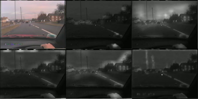
Figure 3: Samples and Saliency Maps of ITT, GBVS, PFT, and PQFT, and ENT methods (left-to-right top-to-bottom order). Please see the supplementary materials for sample sections of the video containing the original scene with the eye fixation marker overlayed on it and saliency maps of various methods.

Though the spatial temporal saliency results seems to fit into context of images, the method has not well optimized and analysed yet. Figure 4, from left to right, shows original image, spatial saliency maps and temporal saliency maps according to conditional entropy or KL divergence estimation values. In this figure, MSF means medium sub-band feature is in use; SSM and TSM represent spatial saliency maps and temporal saliency map respectively; meanwhile, CON and KLD notifies which kdpee entropy estimation mode in used. First, all saliency maps regardless of approaches ( SSM / TSM or CON / KLD ) identifies edges as high saliency regions. Intuitively, edge regions of images witness sharp change in intensity values between pixels as well as large statistical difference between neighbouring blocks in both spatial and temporal domain. Therefore, surrounding information of edge blocks does not provide much information for identification of central block statistical properties; then, large entropy difference occurs at these edge blocks. Secondly, visual results differentiate performance of KLD and CON approaches; KLD method generates less noise saliency map but less contrasting range; whereas, CON saliency map is much more noisy but the contrast range is larger than the previous method. However, both of them are sensitive to noise, or small change in high intensity area for example sky regions. Besides noise levels in KLD and CON maps, another observable point is high similarity between spatial and temporal saliency maps. The high correlation of pixels between successive frames results in a temporal saliency map (TSM) with much similarity to a spatial saliency map (SSM). Current drawbacks of the proposed method are solely due to its sensitivity to noise and correlation between neighbouring data, and these problem can be solved by de-noising and decorrelation technique later introduced.

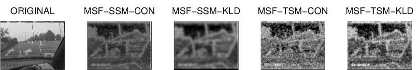
Figure 4: Standard Deviation of Each Sub-band in Camera-man Image

5 Image Patch Data Preprocessing

As mentioned in the previous section, the fast entropy estimation method empirically partition data into normal distributed groups by kd-tree methods and compute entropy by simplified entropy formula given the normality of data distribution. Since multi-dimensional data need to be dealt with, adaptive kd-tree is utilized instead of traditional kd-tree partitioning processes. When input data are multidimensional, the advantage of this adaptive process is allowing data to be split along different dimensional at different levels. Then, instead of partitioning n-dimensional data all together, data can be split sequentially one dimension after another. In order to ensure close approximation of adaptive strategy to normal partition, both correlation between data dimensions and number of dimensions itself need to be as small as possible. Therefore in data preprocessing stage, a decorrelation process is crucial for performance of the entropy estimation as well as the the whole entropy-based saliency approach. Beside correlation between multidimensional data, its noise is another factor which sometimes severely affect the entropy estimation performance, so noise removal techniques should be considered before any estimation is taken place.

5.1 Data Preprocessing - Dimension Reduction && Decorrelation

5.1.1 Principle Component Analysis - Spatial Data Decorrelation

In image processing and computer vision research field, Principle Component Analysis (PCA) is well established as de-factor decorrelation tools for data processing because of its reliable theory and good practical performance for short signals of low-dimensional data. Besides decorrelating data, through the analysis, data dimensions can be reduced by eliminating projected low-energy PCA coefficients. It comes into handy in our since the amount of samples desperately limits the number of data dimensions which can be reliably estimated.

As mentioned in computing approach of spatial saliency map, entropy need to be estimated from high dimensional dataset, the amount of additional entropy for encoding a central patch data given 4-connected surrounding patches, figure 2, need estimating. Conditional approach first carries out estimation of 5-D dataset, $(\textbf{C,N,S,W,E})$, and 4-D dataset, $(\textbf{C,N,S,W,E})$, and then use their difference as saliency values. Since chosen patch size is around 8x8 ( 64 pixels ) or 9x9 ( 81 pixels ), the number of samples are sufficient for 5-D data entropy computation $\mbox{(}number\_of\_samples)>2^{5}$. However, if 8 connection neighbouring patches are considered, the number of maximum dimensions are no longer 5 but 9. Theoretically, at least $2^{9}\mbox{(}pixels/patch)$ or $256x256\text{(}patches)$ would be used; however it is computationally impractical. Therefore, PCA might be brought in so as to decorrelate and simplify multidimensional data. After the analysis, energy and information of patches are squeezed into first few basis, figure 5. Therefore, ony first few PCA basis or features, 4 or 5 first few basis occupies more than $99.8\%$ of the total energy, can safely describe the pre-analysed data points.

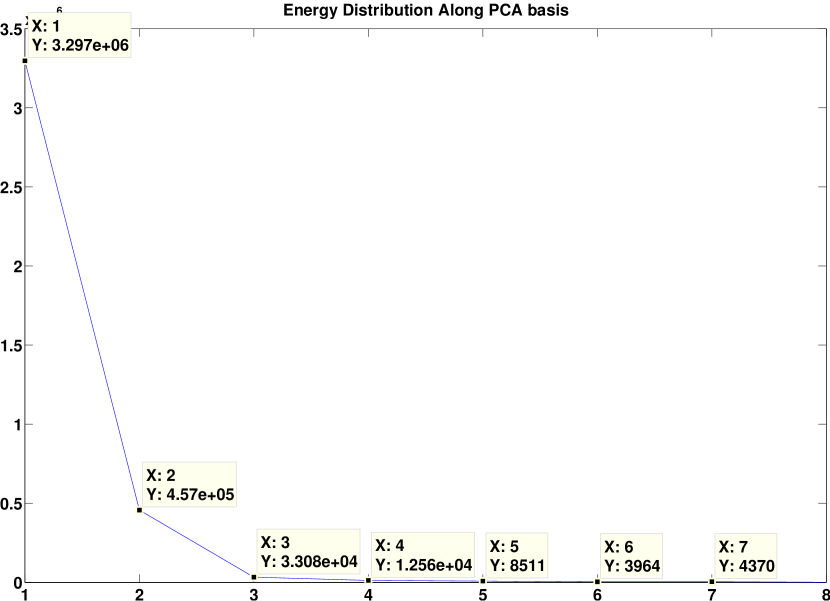
Figure 5: Energy Distribution according to PCA basis

Despite these manifold data, their underlining structure is much more simpler due to high correlation of natural image patches. If this attribute of neighbouring image patches are taken advantage, the manifold data can be much simplified. For example, the fore-mentioned 9-D input dataset might be simplified into much fewer dimensions meanwhile almost all energy of the original signals is reserved; then, only first 4 or 5 basis are enough to capture almost al information. Hence, 8x8 or 9x9 patch size ( 64 or 81 pixels/patch) provides enough data for 9-D kdpee entropy estimation after PCA process is applied. Data, after decorrelated by PCA, helps the adaptive k-d tree method approximately get close to what normal multidimensional k-d tree method might achieve. A small experiment is carried out to compare between between spatial saliency maps generated by the fore-mentioned method with/without decorrelation, 6.

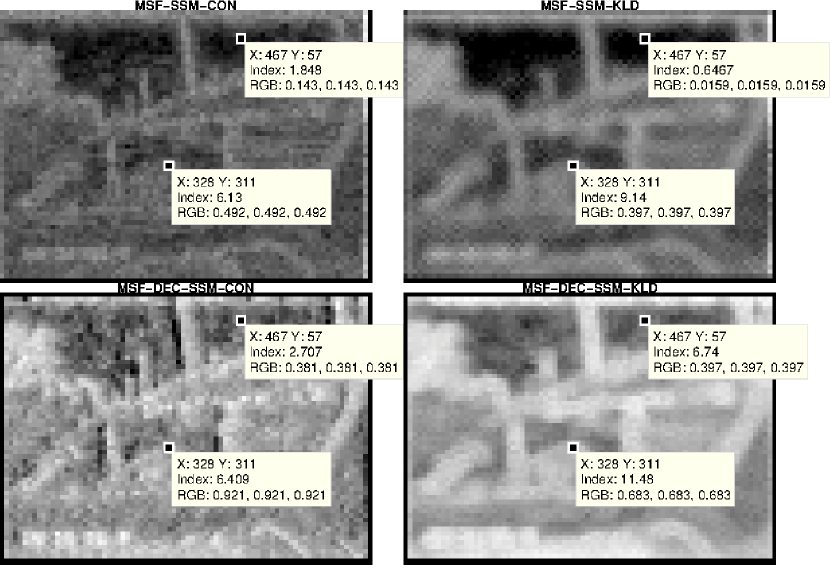
Figure 6: Spatial Saliency Maps by CON and KLD with (the bottom row) / without (the top row) DEC (decorrelation)

The visual results in the figure 6 show that decorrelation steps may not be necessary for the proposed saliency method in spatial domain. Saliency values are collected at two points with following coordinates (328,311) ( edge point ) and (467,57) (sky point). At edge points, saliency values are not much different between methods with or without decorrelation steps. However, the values are significant different on supposedly not salient sky point, and they tend to become bigger at those unimportant positions. Visually, decorrelated data generates more noise on the spatial saliency maps. It seems that 4-connecting neighbours provides better context for spatial saliency entropy estimation than 8-connecting neighbours. Therefore, decorrelation step may not be necessary for spatial saliency map generation. This obviously quite a lot of computational effort because averagely it takes 3 times longer to process data with decorrelating step than without it.

5.2 Discrete Cosine Transform - Temporal Data Decorrelation

Though PCA preferred to be used for decorrelating data and reduce data dimension, it is computationally expensive to carry out that analysis repeatedly. Moreover, temporal data need to be dealt with in this section, and Discrete Cosine Transform (DCT) have strong support as fast alternative for decorrelating temporal data instead of PCA in image and video compression. When there are a lot of movements in the scene like two image sample images on relatively noisy background, first column in the figure 7. The temporal saliency maps generated by prior temporal approach, the middle column of the figure, clearly show that current method can not cope with those noisy signals and their change over time. There is large temporal correlation between pixels of consecutive frames for both salient foreground features and not salient background features. In addition, if a whole stack of consecutive patches of images without preprocessing is utilized for estimating temporal saliency, it partially covers spatial saliency as well since a whole spatial feature data are in use. Meanwhile, interest of temporal saliency method is emphasizing large movement or big difference in pixel values of video frames. Therefore, in order to decorrelate patch data as well as concentrate on motion features, DCT is employed. Besides its decorrelation mentioned before in video compression literature, its 1D computational processes stress on difference of neighbouring values, in this case difference between pixel values of neighbouring frames. Its coefficients eventually resembles changes of frames over time. After applying DCT analysis on MSF features of several frames, the temporal saliency maps become much clearer and they actually highlight moving objects on the table tennis scenes, right column of the figure 7. In addition, the largest coefficients of DCT correlation are removed from temporal saliency estimation in order to limit affects of spatial features on temporal saliency values and noise from background features. Beside removal of the largest component due to its spatial feature, a few smallest DCT coefficients are as well eliminated so as to reduce data dimensions and complexity while its general structure is still intact and meaningful. For example, 8-D data set, composed from 8 consecutive frames, might be simplified into 3-D by removing the first biggest coefficients and the last four smallest coefficients; then the dataset is much simplified and focused on frame differences. The whole temporal decorrelation process is summarized in pseudo-code 1,2. Moreover, it is shown that KLD is better than CON when noise is a major part of image signals, but generally temporal saliency maps are still plagued with noisy non-salient parts. Therefore, de-noising, another preprocessing data step, need integrated besides decorrelating process.

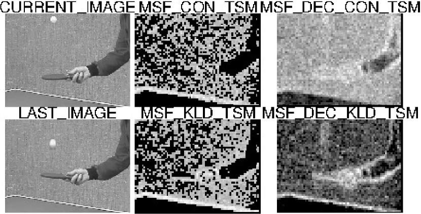
Figure 7: Temporal Saliency Map without / with correlation

Procedure 1 Medium Sub-band Frequency Filter - Temporal Data Decorrelation

0:  $input\_frames$

  $msf3d\_filter\_decorrelation(input\_frames)$

  $wavelet\_coefficients=waveletcdf97(input\_frames,number\_wavelet\_level);$

  $wavelet\_coefficients\{L1\}\leftarrow 0;$ {Assign 0 to all L1 wavelet coefficients}

  $wavelet\_coefficients\{DC\}\leftarrow 0;$ {Assign 0 to all DC wavelet component}

  $dct\_coefficients\_reduced=temporal\_decorrelation(wavelet\_coefficients);$

  $msf\_denoised\_feature=\newline inverse\_waveletcdf97(dct\_coefficients\_reduced,number\_wavelet\_level);$

  $msf\_decorrelated\_feature$

Procedure 2 Temporal Data Decorrelation & Dimension Reduction

0:  $wavelet\_coefficients$

  {Temporal Data Decorrelation Step}

  for $pixel\_counter=1$ to $number\_of\_pixels$ do

     for $frame\_counter=1$ to $number\_of\_frames$ do

        $pixel\_temporal\_data=input\_frames(pixel\_counter,frame\_counter);$

     end for

     $dct\_coefficients(pixel\_counter,:)=dct(pixel\_temporal\_data,:);$

  end for

  {Data Dimension Reduction Step}

  for $pixel\_counter=1$ to $number\_of\_pixels$ do

     for $dct\_basis\_counter=1$ to $number\_of\_dct_{b}asis$ do

        $basis\_energy(dct\_basis\_counter)+=\{dct\_coefficients(pixel\_counter,dct\_basis_{c}ounter)\}^{2};$

     end for

  end for

  {Sort Basis Energy in Descending Order}

  $basis\_energy\_sorted\_index=sort(basis\_energy,^{\prime\prime}descend^{\prime\prime});$

  for $pixel\_counter=1$ to $number\_of\_pixels$ do

     for $index\_counter=2$ to $number\_dct\_basis/2$ do

        $dct\_coeffcients\_reduced(pixel\_counter,basis\_energy\_sorted\_index(index\_counter))\leftarrow dct\_coefficients(pixel\_counter,basis\_energy\_sorted\_index(index\_counter));$

     end for

  end for

  $dct\_coefficients\_reduced$

5.3 Data Preprocessing - Data De-noising

5.3.1 Spatial Saliency Map De-noising

Though in theory MSF features provides suitable data for kdpee estimation due to its freedom from DC signals and noise-rich L1 wavelet features, noise does occurs in other frequency sub-band as well. Therefore, entropy estimation is still sometimes suffered from mixtures of edges and noise well. It leads to over-estimation of spatial entropy and inaccuracy of saliency values. Beside removal of the highest frequency components from wavelet analysis, further technique must be utilized to suppress unwanted noise in the rest of sub-band without need of removing entire frequency spectrum of images signals. Bivariate shrinkage functions, introduced by Sendur et al.Sendur2002 , is employed since its de-noising mechanism operates on wavelet domain. In brief, its noise suppression technique bases on correlation between parents and children wavelet coefficients; that correlation implies the wavelet coefficients have high possibility of belonging to salient edges feature if its parent coefficients are extracted from edge features and vice versa. In other words, bivariate shrinkage reserves coefficients which are salient across several scales or sub-band and eliminate noise features which are often only salient in a specific scale. The spatial denoise program is described in pseudo-code 3.

Procedure 3 Medium Subband Frequency Filter - Bivariate Shrinkage De-noising

0:  $input\_image,number\_wavelet\_level$

  $wavelet\_coefficients=waveletcdf97(input\_image$,$number\_wavelet\_level);$

  $wavelet\_coefficients\{L1\}\leftarrow 0;$

  $wavelet\_coefficients\{DC\}\leftarrow 0;$

  $denoised\_wavelet\_coefficients=\newline bivariate\_shrinkage$($wavelet\_coefficients,number\_wavelet\_level-1);$

  $msf\_denoised\_feature=inverse\_waveletcdf97(input\_image,number\_wavelet\_level);$

  $msf\_denoised\_feature$

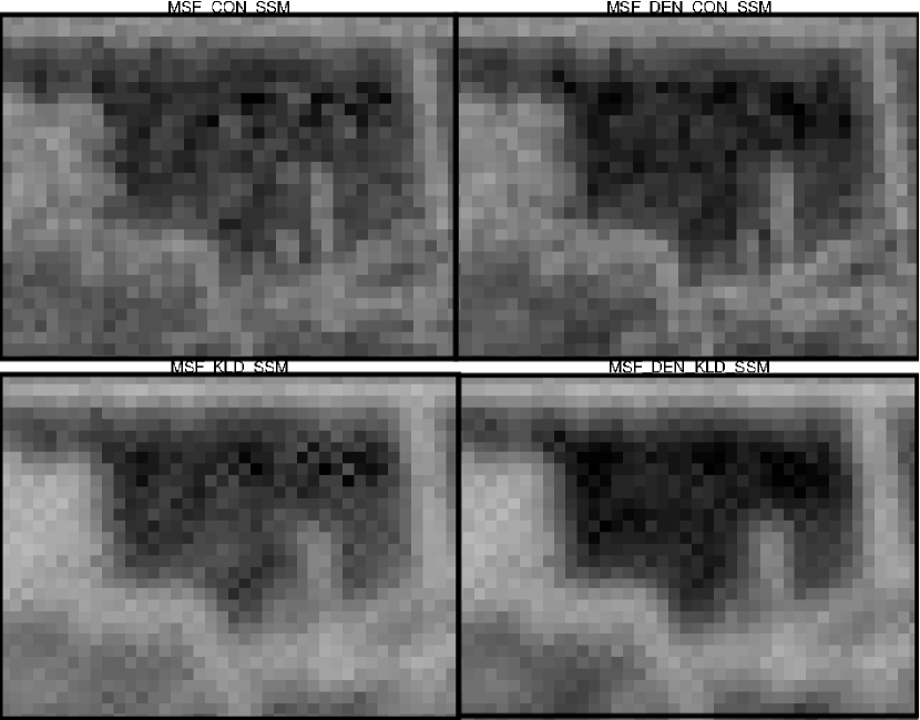
Figure 8: Spatial Saliency Map: (left) without denoising, (right) with denoising

De-nosing effect on spatial saliency maps can be seen on spatial saliency maps of the figure 8. It shows saliency maps generated by CON (top row), KLD (bottom row) with de-noising affect ( left column ) and without denoising affect ( right column ). Its affect can be clearly observed on the bottom row, applying bivariate shrinkage before saliency value KLD estimation technique generates smooth and nearly free noise spatial saliency maps. Especially this de-noising incorporated well into the previous MSF feature extraction because it reuses wavelet CDF 9/7 analysed coefficients. Therefore, it does not requires much addition computational effort. Due to its good performance and, that bivariate shrinkage might be extended to suppress noisy temporal saliency maps, the figure 7

5.3.2 Temporal Saliency Map De-noising

Previous sections have already elaborated about how bivariate shrinkage technique removes noise in spatial saliency map. As fore-mentioned, the DCT biggest basis and a few smallest basis are eliminated to avoid spatial features and reduce data complexity. However, their saliency maps are still affected by noise which exist in the rest of DCT basis. Bivariate shrinkage suppress noise on each DCT basis by using correlation between parent and children wavelet coefficients, pseudo-code 4.

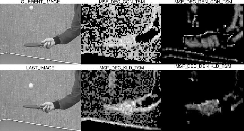
Figure 9: Spatial Saliency Map: (left) without denoising, (right) with denoising

Table tennis samples are again used to demonstrate how much noise can be removed from temporal saliency maps after bivariate shrinkage approach. Almost all background noise have been removed from the saliency maps as illustrated in the left-most column of the figure 9 9. Both CON and KLD successfully highlights supposedly saliency objects on the scene which are moving table tennis balls, and arms of players.

Procedure 4 Medium Sub-band Frequency Filter - Temporal Data Decorrelation & Denoisation

0:  $input\_frames$

  $msf3d\_filter\_decorrelation(input\_frames)$

  $wavelet\_coefficients=waveletcdf97(input\_frames,number\_wavelet\_level);$

  $wavelet\_coefficients\{L1\}\leftarrow 0;$

  $wavelet\_coefficients\{DC\}\leftarrow 0;$

  $dct\_coefficients\_reduced=temporal\_decorrelation(wavelet\_coefficients);$

  for $dct\_basis\_counter=1$ to $number\_of\_dct\_basis\_reduced$ do

     $dct\_coefficients\_reduced\_denoised=\newline bivariate\_shrinkage(dct\_coefficients\_reduced,number\_wavelet\_level-1);$

  end for

  $msf\_denoised\_feature=\newline inverse\_waveletcdf97(dct\_coefficients\_reduced,number\_wavelet\_level);$

  $msf\_decorrelated\_feature$

6 Experimental Results

We evaluate the new conditional entropy based saliency method (from now on referred to as ENT) on publicly available eye tracking databases of Bruce and Tsotos Bruce2006b and Judd et al.Judd2009 , and compare it with a number of saliency estimation methods in the literature including, Itti and Koch (ITT) itti1998model , spectral residual saliency (SRS) Hou2007 , phase frequency transform (PFT) and phase quaternion frequency saliency (PQFT) Guo2008 , Information Maximization (AIM)Bruce2006b , and discriminant saliency (DIS) Gao2007 . Among these saliency methods, PQFT and the proposed method incorporate both spatial and temporal information meanwhile, others solely generate saliency maps in frame-by-frame manner. Therefore, experiments on both spatial and spatio-temporal data are in need.

6.1 Spatial Expeiments

In Bruce’s image database Bruce2009a , eye tracking data were collected from 20 human subjects over 120 different colour images. Scenes of these photos include both outdoor and indoor environment, some contain very clear and big salient objects, but some contain a variety of small objects. This image database has been used by the data originator and a number of other researchers for evaluating saliency estimation methods.

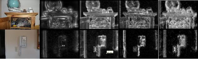
Figure 10: Examples of Saliency Maps of ITT, AIM, and the new ENT methods (left-to-right)

Figure 10 shows the saliency maps of a number of example images generated by different methods. It is seen that the visual appearance of these saliency maps are quite similar.

To compare the performances of different methods quantitatively, we can use Tatler’s numeric measurement Tatler2005 . The saliency maps are treated as binary classifiers to discriminate fixation points versus non-fixation points. The threshold for classifying fixation points are not fixed but systematically changed from the minimum to the maximum of the saliency maps to generate ROC curves. The ROC curves of various methods tested on Bruce’s database Bruce2009a are shown in Figure 11. The area under the ROC curves (AUC) have been used by a number of authors to give quantitative comparison of saliency computation methods and table 2 shows the AUC values of five different methods.

Table 2: Area Under Curve (AUC) for different methods.

Methods	ITT itti1998model	AIM Bruce2006b	ENT-CON	ENT-KLD	DISGao2007	SRSHou2007
AUC	0.70947	0.73873	0.78167	0.73280	0.76940	0.75434

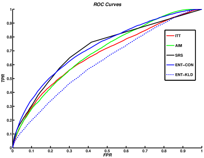
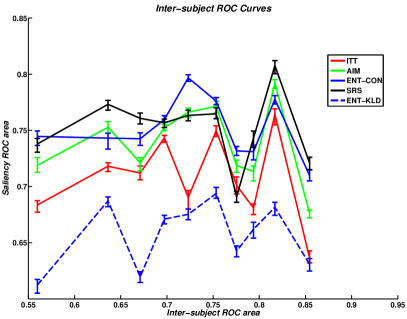
Figure 11: ROC and Inter-subject ROC curves of ITT, AIM, and ENT-CON/KLD

The ROC curves show that the new ENT-CON method generally performs better than AIM and ITT methods, and the performances are reconfirmed by the area under curve (AUC) results in table 2. In the table, the AUC result of DIS saliency method was performed on the same database by the original authors and taken directly from Gao2007 . These AUC results show that ENT methods also performs better or at least as good as the DIS method.

ROC curves and AUC values are useful for comparing different computational saliency approaches, but they do not show relation between these methods with human performance. The inter-subject ROC curves performance evaluation methods proposed by Harel et al.Harel2007a helps to show performance of human visual system versus that of computational saliency method: for each image, a mean inter-subject ROC area was computed as follows: for each of the subjects who viewed an image, the fixation points of all other subjects were convolved with a circular, decaying kernel with decay constant matched to the decaying cone density in the retina. This was treated as a saliency map derived directly from human fixations, and with the target points being set to the fixations of the chosen subject, an ROC area was computed for a single subject. The mean over all subjects is termed ”inter-subject ROC value”. For any particular computational scheme, an ROC area was computed using the resulting saliency map together with the fixations from all human subjects as target points to detect. The inter subject ROC values are shown in Figure 11. This plot clearly demonstrates that our new ENT technique has outperformed current state-of-art saliency methods and displayed a good matching with human-eye fixation points.

Table 3: Time Consumption of Saliency Methods

Methods	ITT	AIM	ENT-CON	ENT-KLD	SRS
Time (s)	1.2488	66.2673	0.93094	0.56824	0.33654

Information-theoretic saliency methods such as AIM has disadvantages due to its massive computational requirements which are not suitable for realtime applications. Therefore, in addition to an accuracy requirement, the proposed method aims to achieve computational efficiency. Table 3 shows the computational speeds of several techniques, it is seen that ENT is over 70 times faster than AIM method and 1.3 times faster than ITT method, noted that only the spatial map of the proposed method is generate to be fair in speed comparisons with other frame-by-frame based saliency method. Though it is slower than SRS method, ENT can better match eye-fixation data than SRS. All experiments are done using MATLAB 2010b in a 2.33 GHz Intel Core 2 Duo computer running Linux Ubuntu 10.10 OS.

Table 4: Area Under Curve (AUC)

Methods	ITT	AIM	ENT-CON	MITJudd2009
AUC	0.74940	0.71165	0.78157	0.68845

We have also tested our method on the database created by Judd et al.Judd2009 . This database has 1003 photos with eye fixation data from 15 viewers, and the database was used for evaluating Judd’s learning based saliency method. We carried out similar qualitative and quantitative evaluation as Judd2009 on the 100 testing images used in the original paper. Visual illustration of a sample photo and its saliency maps of ITT, AIM, ENT and MITJudd2009 is shown in the figure 12. Quantitative results are shown in the table 4 which again show that the new ENT-CON method compares very well against other methods.

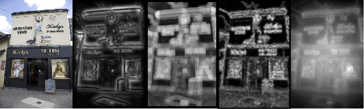
Figure 12: Samples and Saliency Maps of ITT, AIM, ENT, and MIT methods (left-to-right order)

6.2 Spatiotemporal Experiments

Aforementioned experiments only focus on current frame information or spatial side of available information; however, the proposed ENT method is naturally extended to estimating saliency from temporal information of available data as well, introduced in the section 4. For quantitative performance evaluation and comparisons of the spatiotemporal and spatial saliency methods, simulations must be done only spatiotemporal input data; in other words, video materials. Moreover, this paper focuses in specific video context, human visual perception in driving contexts; therefore, the supplementary video data must be recorded in drivers’ point of views and psychological related data eye-fixation or ground truth segments done by human beings. Following these criteria, there are two video database put in use, AUTOM and MSDR Brostow2008 . AUTOM database includes a round 10 minutes videos, recored by a camera on head-mounted eye-trackers which at the same time detect drivers’ fixation points on road scenes. Meanwhile, MSDR is as well recorded on road with drivers’ view in high resolution but it has ground truth for each frame instead of eye-fixation data. Experiments on AUTOM database emphasizes correlation between artificial saliency maps of different computational method with human psychological data; meanwhile, MSDR with ground truths for specific purposes stresses on specific application how well saliency maps relates to important features in the scenes.

6.2.1 AUTOM database

The AUTOM video database is created by Accident Research Unit, the University of Nottingham, UK Campus, which includes 28 short segmented videos; each has 500 frames except the last video which has 512 frames. The whole video database has 14012 frames which lasts for 9 minutes and 20 seconds. These videos are recorded with a head-mounted camera of SMI eye-trackers; simultaneously, two small cameras, pointing to pupils of the driver’s eyes, locate drivers’ eye fixation at 250 Hz. The videos are recorded in real-life driving situations; therefore, several road types and traffic situations have been covered such as urban roads, high ways, speeding up and slowing down situations. It does not extensively covers all possible driving schemes, but it provides sufficient materials about human eye-fixation in most daily driving situations. Importantly, each frame of these videos are recorded with drivers’ eye fixation response to specific real-life driving situations. Different from previous ways of collecting multiple eye-fixation data for each static picture, there is only one eye-fixation position data for each frame. The data format is changed, so are evaluation methods since ROC, AUC and ISROC are not suitable for the evaluation of video with eye-marks.

In saliency literature, Normalized Saliency Value (NSV) and Chance Adjusted Saliency (CAS) have been proposed for correlating human performance and generated saliency maps spatiotemporally.

Table 5: Normalized Saliency Value

Observations	ITTI	GBVS	PFT	PQFT	ENT-CON	ENT-KLD
sample_00	0.026	0.39	0.145	0.146	0.398	0.596
sample_01	0.018	0.339	0.131	0.136	0.318	0.444
sample_02	0.033	0.359	0.156	0.156	0.489	0.671
sample_03	0.028	0.406	0.185	0.195	0.556	0.708
sample_04	0.01	0.306	0.099	0.1	0.242	0.348
sample_05	0.029	0.28	0.08	0.088	0.209	0.271
sample_06	0.028	0.29	0.096	0.122	0.254	0.364
sample_07	0.008	0.371	0.125	0.164	0.267	0.39
sample_08	0.022	0.378	0.141	0.161	0.323	0.468
sample_09	0.014	0.433	0.156	0.169	0.411	0.548
sample_10	0.002	0.306	0.077	0.096	0.145	0.24
sample_11	0.015	0.336	0.107	0.101	0.241	0.341
sample_12	0.034	0.387	0.139	0.13	0.369	0.545
sample_13	0.015	0.38	0.142	0.134	0.338	0.435
sample_14	0.017	0.381	0.215	0.163	0.564	0.69
sample_15	0.064	0.409	0.174	0.185	0.563	0.704
sample_16	0.024	0.257	0.082	0.101	0.216	0.353
sample_17	0.027	0.527	0.231	0.271	0.555	0.736
sample_18	0.022	0.423	0.157	0.198	0.327	0.442
sample_19	0.065	0.286	0.06	0.103	0.159	0.24
sample_20	0.123	0.423	0.123	0.175	0.363	0.582
sample_21	0.16	0.374	0.118	0.151	0.36	0.61
sample_22	0.059	0.341	0.099	0.157	0.282	0.456
sample_23	0.077	0.354	0.135	0.155	0.355	0.643
sample_24	0.048	0.411	0.177	0.189	0.409	0.589
sample_25	0.069	0.389	0.194	0.192	0.475	0.695
sample_26	0.019	0.415	0.238	0.239	0.482	0.628
sample_27	0.097	0.418	0.243	0.244	0.558	0.746
Samples	0.041	0.37	0.144	0.158	0.365	0.517

Normalized Saliency Value is in fact collecting saliency values of normalized saliency maps at locations of eye-fixations; the larger NSV is, the more accurate saliency methods can predict human attention points. However, if the saliency values is directly retrieved at locations of eye-marks, they are prone to a mean spatial error of eye-trackers usually $0.5^{\circ}-1^{\circ}$. So as to eliminate those errors, the maximum saliency value in square areas ,whereof center is the fixation point, is chosen instead. In the table 5, a row $Sample_{\#\#}$ represents normalized saliency values of the $\#\#^{th}$ video in the database with respect to six different saliency approaches. The normalized saliency values in each video are calculated by averaging these of all its frames. Last row shows averagely how much saliency values at eye-fixations are in consideration of the whole 10 minutes videos. Averagely, either conditional entropy or Kullback-Leibler saliency methods outperform the other state-of-the-art approaches. Second to our method in average NVS values is GBVS method, then PQFT, PFT and ITT saliency methods are ranked in descending orders.

Table 6: Chance Adjusted Saliency

Observations	ITTI	GBVS	PFT	PQFT	ENT-CON	ENT-KLD
sample_00	-0.01620	0.15105	-0.01912	-0.02068	0.09810	0.16031
sample_01	-0.02883	0.10282	-0.05274	-0.05878	-0.00154	-0.01592
sample_02	-0.00547	0.13573	-0.03199	-0.03077	0.16424	0.20673
sample_03	-0.01498	0.19607	0.03642	0.02633	0.27253	0.29317
sample_04	-0.03208	0.08501	-0.08824	-0.08548	-0.07596	-0.10103
sample_05	-0.01848	0.05986	-0.11093	-0.08703	-0.09415	-0.15169
sample_06	-0.02129	0.07737	-0.05542	-0.04822	-0.03347	-0.04137
sample_07	-0.02886	0.12561	-0.04424	-0.04983	-0.06474	-0.06572
sample_08	-0.01703	0.13734	-0.04811	-0.04805	-0.01329	0.01062
sample_09	-0.02898	0.18808	-0.03441	-0.04354	0.04525	0.06153
sample_10	-0.04026	0.08053	-0.11124	-0.12110	-0.22137	-0.26291
sample_11	-0.02833	0.09366	-0.09500	-0.08694	-0.07029	-0.10209
sample_12	-0.00883	0.16270	-0.03029	-0.03776	0.07808	0.12318
sample_13	-0.02912	0.16786	-0.02083	-0.02337	0.04448	0.02625
sample_14	-0.02420	0.15050	0.01061	-0.02473	0.22266	0.22460
sample_15	0.01803	0.17338	-0.00786	0.00165	0.24206	0.26677
sample_16	-0.01952	0.05000	-0.08519	-0.07502	-0.08264	-0.06527
sample_17	-0.01150	0.27638	0.03338	0.09682	0.25085	0.28031
sample_18	-0.02229	0.16684	-0.02129	0.00881	0.03661	0.00775
sample_19	0.01972	0.07822	-0.08941	-0.07300	-0.10352	-0.16421
sample_20	0.08400	0.21136	-0.01114	0.00762	0.10156	0.16437
sample_21	0.11576	0.20080	-0.00166	0.00948	0.12431	0.24193
sample_22	0.01808	0.13805	-0.01966	-0.01490	0.02612	0.06633
sample_23	0.03123	0.14159	-0.01558	-0.02963	0.05672	0.20264
sample_24	0.00010	0.22466	0.03073	0.01936	0.14511	0.18615
sample_25	0.02951	0.19172	0.03718	0.03137	0.21777	0.30256
sample_26	-0.02134	0.18658	0.07070	0.05061	0.18509	0.19666
sample_27	0.05362	0.21951	0.09223	0.05795	0.28961	0.34264
Samples	-0.00170	0.14905	-0.02440	-0.02317	0.06572	0.08551

Chance-adjusted saliency performance metric proposed by Parkhurst et al.Parkhurst2002a emerged in the literature as the preferred metric for saliency method comparisons. It basically measure difference in correlation of each saliency method between fixation points generated by human visual systems and random number generators. The more significant the difference (CAS) is, the better saliency maps can distinguish between human eye fixations and randomly generated fixations. In the table 6, GBVS saliency method has more success averagely than other saliency methods in distinguishing between human and random eye-fixations. Second to GBVS are our proposed methods ENT-CON and ENT-KLD, then ITTI, PFT and PQFT are ranked in descending order.

Looking at descending orders in performance according to NSV and CAS of saliency methods $R_{NSV}=\{ENT-KLD,ENT-CON,GBVS,PQFT,PFT,ITTI\}$ and $R_{CAS}=\{GBVS,ENT-KLD,ENT-CON,ITTI,PQFT,PFT\}$, we can make conclusions that groups of saliency methods GBVS, ENT-KLD and ENT-CON outperforms the other group PQFT,PFT, and ITTI. However, there is discrepancy inside each group when choosing CAS or NSV as evaluating methods. In a superior group, our proposed method generates saliency maps with more specific local details than GBVS does. That is a reason why ENT-KLD / ENT-CON performs better than GBVS in NSV but worse than GBVS in CAS. In order to make the comparison fairer between local feature saliency methods and their global counterparts, region of interest mask are applied on local saliency maps. The ROI masks are simply generated by setting threshold on saliency values. Similar explanation can be used for discrepancy in CAS, and NSV results of inferior group of saliency methods.

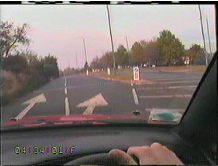
(a) go_alone

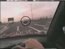
(b) follow_car

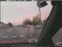
(c) slow_down

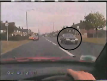
(d) go_toward

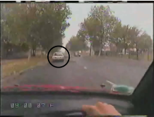
(e) go_away

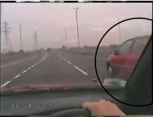
(f) overtake

Figure 13: Attention maps generate by six different methods

Table 7: Normalized Saliency Values in various driving contexts

Observations	ITTI	GBVS	PFT	PQFT	ENT-CON	ENT-KLD
go_alone	0.01851	0.33936	0.14633	0.13281	0.37296	0.49269
head_toward	0.02014	0.38734	0.15944	0.16283	0.45549	0.60256
go_away	0.06923	0.36038	0.11404	0.14979	0.28620	0.45065
overtake	0.07783	0.43606	0.14036	0.19497	0.43177	0.59839
slow_down	0.02451	0.41908	0.16767	0.16924	0.45894	0.59269
follow_car	0.03816	0.37397	0.16606	0.16504	0.36305	0.52260
Mean	0.04140	0.38603	0.14898	0.16245	0.39473	0.54326
Variance	0.00056	0.00110	0.00034	0.00036	0.00374	0.00343

Table 8: Difference in Normalized Saliency Values between go_alone and others

Observations	ITTI	GBVS	PFT	PQFT	ENT-CON	ENT-KLD
go_alone	0.00000	0.00000	0.00000	0.00000	0.00000	0.00000
head_toward	0.00146	0.04781	0.01294	0.02982	0.01619	0.02730
go_away	0.04952	0.02009	-0.03281	0.01635	-0.01624	-0.00526
overtake	0.04721	0.04149	0.01184	0.03407	0.00109	0.05625
slow_down	0.00996	0.02267	0.01569	0.04101	0.01768	0.05115
follow_car	0.01574	0.04859	0.00204	0.02750	-0.00926	-0.01375
Mean	0.02065	0.03011	0.00162	0.02479	0.00158	0.01928
Variance	0.00041	0.00031	0.00027	0.00018	0.00015	0.00075

Besides the studies in general driving scenes, statistical correlation between saliency maps and human response to specific driving situations are interested as well. It helps answer the question how specific driving situations may affect relations between saliency maps and human eye fixations. Does that correlation get better or worse generally ? Before answering this question, we need to specify available specific driving contexts available in our recorded data, and the number of frames in the situations should be large enough to ensure the relative generality of our experiments. After skimming throughout the database, there are six significant specific driving situations: go_alone, go_toward, go_away, slow_down, overtake and follow_car. These situations are named after main tasks which drivers carry out; for example, go_alone, slow_down and follow_car are used to describe situations wherein a car is driven alone without any other moving objects on roads - the figure 13a, is slowed down when reaching a street corner - the figure 13c, and the driver follows a car in front - the figure 13b. Likewise, go_toward or go_away are used for in-front cars which are moving toward the driver ’s car - the figure 13d, or moving away the driver’s car - the figure 13e. Similarly, overtake is named after the situation wherein behind cars suddenly overtake the driver’s car - the figure 13f. In the go_alone context, there are no dynamically moving object on roads, so it should have less visually salient objects and values at eye-marks of those scenes. In other words, the normalized saliency values of go_alone should be less than any other cases. The table 8 summarized differences in normalized saliency values at human fixation points, the table 7, between go_alone and other driving situations. Almost all values in the table 8 is positive, which means increment in performance of saliency methods whenever drivers are found in particular traffic situations rather than being alone on the roads. Expectingly, the ENT-KLD and ENT-CON saliency method still possesses the best normalized saliency values in the table 7, and its performance in specific driving contexts are generally better than go_alone situations; there are some decrements in some specific situations because of shortage of frames in that context. More video samples need to be collected and analysed later to clearly find out how saliency maps and human eye-fixations are related in a particular situation. In the constrained number of input video samples and experiments, saliency methods and human psychological data generally have more match in specific driving situations than being alone on the roads.

Figure 14: Samples and Saliency Maps of ITT, GBVS, PFT, and PQFT, and ENT methods (left-to-right top-to-bottom order). Please see the supplementary materials for sample sections of the video containing the original scene with the eye fixation marker overlayed on it and saliency maps of various methods.

6.2.2 MSRD Database

In the previous AUTOM database section, there are a few studies which mainly focus on psychological fitness aspect of computational saliency maps by usage of eye-fixation data. In this section, a study focusing on application aspect of saliency approaches is done on Motion-based Segmentation and Recognition dataset (MSRD) Brostow2009 with their ground-truth data; figure 15 reveals a sample of a video from MSDR database with its ground truth.

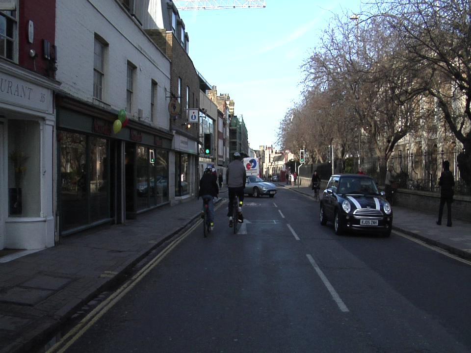
(a) Sample Image

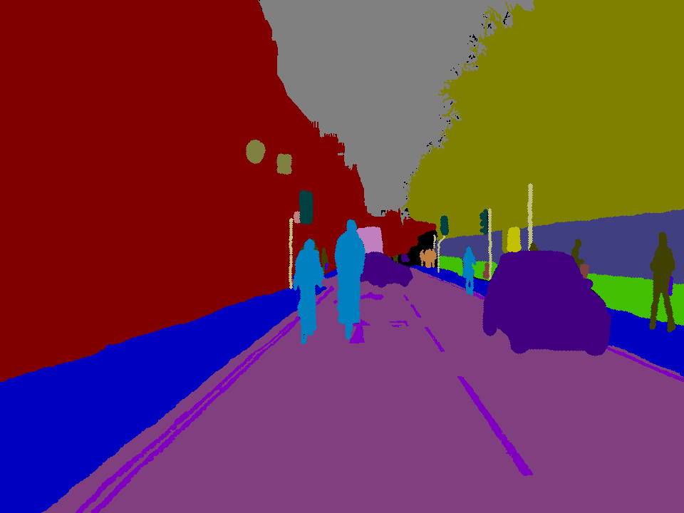
(b) Ground Truth

(c) Importance Map

Figure 15: MSDR Data Samle Image, Ground Truth

Before diving into specific details of the study and its evaluation, I need to briefly describe the MSRD data and reasons why it is chosen to be studied. Another name of MSRD database is Cambridge-driving Labeled Video Database (CamVid) which is a collection of driving context videos with object class semantic metadata. It provides groud truth labels that associate each pixel with one of 32 semantic classes. Contrary to majority of traffic database which is recorded from CCTV camera, it uses similar approach to aforementioned AUTOM database which capture video data from the perspective of an automobile driver. Moreover, the driving scenarios are increasingly complex and filled with a large number and heterogeneity of objects in daily driving scenes. Wide range of objects appears in frames is suitable for our study of saliency maps in general driving scenarios. MSRD database provides over ten minutes of high quality 30 Hz footage wherein some parts are semantically labelled at 1Hz and 15Hz. Totally, ground truth data of over 700 images are manually specified by the first human observer and reconfirmed by the second subject for accuracy. Though videos of the whole database last for ten minutes, only 700 sample frames with their correspondent ground truth data are useful in our studies. In addition to 700 frames extracted from original video at 1Hz or 15Hz, four of their past frames are acquired to serve as input data for spatio-temporal saliency maps.

In MSRD dataset, ground truth data of each sample is a map of manually classified objects wherein each pixel belongs to one of 32 available classes. For a specific application, a certain class of objects will be more important than others. For instance, pedestrians classes bears the most importance values in pedestrian detection applications. Our studies about general driving context and safety leaves us with a certain scale of importance for 32 available classes. Among available classes, there are roughly four groups of objects: the moving objects group, .i.e pedestrian, children, the road objects group, .i.e road, roadshoulder, ceiling objects group, sky, tunnel, and fixed objects group, building, wall, tree. Generally in driving situations, those groups can be arranged in descending order of their importance as moving objects, road objects, fixed objects, and ceiling objects group. Inside each group, object classes are ranked for its importance in the scene; then, we will have importance score for every available object class in the table 9.

Table 9: Importance order of MSRD object classes

Moving objects	Imp	Road objects	Imp	Fixed objects	Imp
Child	32	Road	18	TrafficLight	17
Pedestrian	31	RoadShoulder	19	SignSymbol	16
Animal	30	LaneMkgsDriv	20	TrafficCone	15
Bicyclist	29	LaneMkgsNonDriv	21	Column_Pole	14
MotorcycleScooter	28	Ceiling objects	Imp	Sidewalk	13
CartLuggagePram	27	Archway	3	Bridge	12
Car	26	Tunnel	2	ParkingBlock	11
SUVPickupTruck	25	Sky	1	Misc_Text	10
Truck_Bus	24			Building	9
Train	23			Fence	8
Misc	22			Wall	7
				Tree	6
				VegetationMisc	5
				Void	4

Using the table 9, image pixels of specific classes in the ground truth data can be mapped to its corresponding importance values. In other words, importance maps can be constructed from ground truth data of MSRD dataset. Currently, each pixel in importance maps have integer values in the range of $[1,32]$, while saliency values are decimal numbers in the range $[0,1]$. Then values of importance maps need scaling down to $[0,1]$ to ensure reliability of further evaluations.

Normalized importance maps shows us how relatively vital each pixel on that map is our purposes, and we also want to know whether higher saliency values in saliency maps means that pixels is more meaningful and necessary to our purposes or not. That leads use to the question how well correlated normalized importance maps and normalized saliency maps are. The normalized cross correlation is chosen to measure and demonstrate that relation. Lets assumed that there are a saliency map $S$ in short of $S(x,y)$ and importance map $M$ in short of $M(x,y)$, the normalized cross correlation $NORMXCORR$ is formulated as the equation 13, and its range of value is $[-1,1]$.

$$NORMXCORR=\frac{\sum_{x,y}[S-\mu(S)][M-\mu(M)]}{(\sum_{x,y}[S-\mu(S)]^{2}\sum_{x,y}[M-\mu(M)]^{2})^{\frac{1}{2}}}$$ (13)

Among over 700 useful data images, they belong to three video scenes. In order to save space and generalize the simulation results, NORMXCORR of frames from three video sequences will be plotted in three figures: figure 16,17,18. Each figure has six lines with different colour representing NORMXCROSS between importance maps and saliency maps from six saliency methods over frames of a sequence. The plots show how the measurement fluctuate and change across the whole video, and their statistical mean and variance are also displayed in the tables 10, 11, 12.

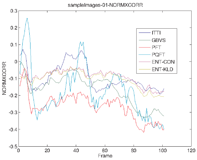
Figure 16: Normalized Cross Correlation for sequence_01

Table 10: Statistical data of Normalized Cross Correlation over video sequence 01

Observations	ITTI	GBVS	PFT	PQFT	INFO	ENTRO
Mean	-0.09315	-0.16580	-0.26443	-0.17535	-0.09301	-0.10431
Variance	0.00615	0.00775	0.00620	0.02255	0.00188	0.00248

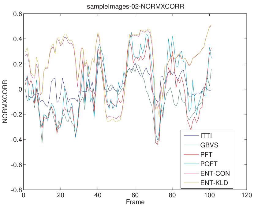
Figure 17: Normalized Cross Correlation for sequence_02

Table 11: Statistical data of Normalized Cross Correlation over video sequence 02

Observations	ITTI	GBVS	PFT	PQFT	INFO	ENTRO
Mean	0.02512	-0.08502	-0.03021	0.02062	0.20900	0.21499
Variance	0.00866	0.02305	0.04298	0.04906	0.04088	0.04544

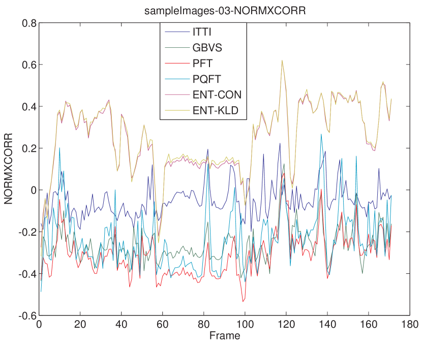
Figure 18: Normalized Cross Correlation for sequence_03

Table 12: Statistical data of Normalized Cross Correlation over video sequence 03

Observations	ITTI	GBVS	PFT	PQFT	INFO	ENTRO
Mean	-0.04801	-0.26006	-0.30763	-0.23102	0.24872	0.25500
Variance	0.00638	0.00763	0.01083	0.01970	0.02723	0.02761

After looking through three plots and three tables, NORMXCROSS of the proposed method is larger than the other established methods. Though in some psychological measurements, the proposed ENT method does not give the best performance, its saliency maps are well correlated with application oriented importance maps; in other words, it provides clues about how important and meaningful each pixel is to the scene.

7 Concluding Remarks

In this paper, we have formulated bottom-up visual saliency as center surround conditional entropy and presented a fast and efficient computational method for computing saliency maps on still images and full motion videos. We have shown that the new method is not only computationally fast and efficient but also gives state of the art performances on publicly available eye tracking databases. Furthermore, the technique is feasibly extended from still image saliency, spatial saliency, to video data, spatial temporal saliency, and its efficiency is evaluated on two driving context video database AUTOM and MSRD. As visual saliency is a bottom-up as well as a top-down process, our future work will investigate the including of top-down context in the estimation of visual saliency and explore its various applications in various cognitive researches.

References

- (1) Brostow, G.J., Fauqueur, J., Cipolla, R.: Semantic object classes in video: A high-definition ground truth database. Pattern Recognition Letters 30(2), 88–97 (2009). DOI 10.1016/j.patrec.2008.04.005
- (2) Brostow, G.J., Shotton, J., Fauqueur, J., Cipolla, R.: Segmentation and Recognition using Structure from Motion Point Clouds pp. 1–14 (2008)
- (3) Bruce, N., Tsotsos, J.: Saliency based on information maximization. Advances in neural information processing systems 18, 155 (2006)
- (4) Bruce, N.D.B., Tsotsos, J.K.: Saliency , attention , and visual search : An information theoretic approach. Journal of Vision 9, 1–24 (2009). DOI 10.1167/9.3.5.Introduction
- (5) Cohen, A., Daubechies, I., Feauveau, J.C.: Biorthogonal bases of compactly supported wavelets. Communications on Pure and Applied Mathematics 45(5), 485–560 (1992)
- (6) Gao, D., Mahadevan, V., Vasconcelos, N.: The discriminant center-surround hypothesis for bottom-up saliency. Advances in Neural Information Processing Systems 20, 1–8 (2007)
- (7) Guo, C.L., Ma, Q., Zhang, L.M.: Spatio-temporal Saliency detection using phase spectrum of quaternion fourier transform. IEEE (2008). DOI 10.1109/CVPR.2008.4587715
- (8) Harel, J., Koch, C., Perona, P.: Graph-based visual saliency. Advances in neural information processing systems 19, 545 (2007)
- (9) Hou, X., Zhang, L.: Saliency detection: A spectral residual approach. In: IEEE Conference on Computer Vision and Pattern Recognition (CVPR07). IEEE Computer Society, 800, pp. 1–8. Citeseer (2007). DOI 10.1109/CVPR.2007.383267
- (10) Hubel, D.H., WIESEL, T.N.: Receptive fields and functional architecture into nonstriate visual areas (18 and 19) of the cat. Journal of neurophysiology 28, 229–89 (1965)
- (11) Itti, L., Baldi, P.: Bayesian surprise attracts human attention. Advances in neural information processing systems 18, 547 (2006)
- (12) Itti, L., Koch, C., Niebur, E.: A model of saliency-based visual attention for rapid scene analysis. IEEE Transactions on pattern analysis and machine intelligence 20(11), 1254–1259 (1998)
- (13) Judd, T., Ehinger, K., Durand, F., Torralba, A.: Learning to predict where humans look. 2009 IEEE 12th International Conference on Computer Vision pp. 2106–2113 (2009). DOI 10.1109/ICCV.2009.5459462
- (14) Parkhurst, D., Law, K., Niebur, E.: Modeling the role of salience in the allocation of overt visual attention. Vision Research 42(1), 107 – 123 (2002)
- (15) Qiu, G., Gu, X., Chen, Z., Chen, Q., Wang, C.: An information theoretic model of spatiotemporal visual saliency. In: to appear, international conference on multimedia and expo, pp. 1806–1809. Citeseer (2007)
- (16) Sendur, L., Selesnick, I.: Bivariate shrinkage with local variance estimation. IEEE Signal Processing Letters 9(12), 438–441 (2002). DOI 10.1109/LSP.2002.806054
- (17) Stowell, D., Plumbley, M.: Fast Multidimensional Entropy Estimation by $ k $-d Partitioning. Signal Processing Letters, IEEE 16(6), 537–540 (2009)
- (18) Tatler, B.W., Baddeley, R.J., Gilchrist, I.D.: Visual correlates of fixation selection: effects of scale and time. Vision research 45(5), 643–59 (2005). DOI 10.1016/j.visres.2004.09.017
- (19) Urban, F., Follet, B., Chamaret, C., Meur, O., Baccino, T.: Medium Spatial Frequencies, a Strong Predictor of Salience. Cognitive Computation (2010). DOI 10.1007/s12559-010-9086-8
- (20) Viola, P., Wells III, W.: Alignment by maximization of mutual information. In: iccv, vol. 24, p. 16. Published by the IEEE Computer Society (1995)