Recently, it was realized that quantum states of matter can be classified as long-range entangled (LRE) states (i.e. with non-trivial topological order) and short-range entangled (SRE) states (i.e. with trivial topological order). We can use group cohomology class ${\cal H}^{d}(SG,\mathbb{R}/\mathbb{Z})$ to systematically describe the SRE states with a symmetry $SG$ [referred as symmetry-protected trivial (SPT) or symmetry-protected topological (SPT) states] in $d$-dimensional space-time. In this paper, we study the physical properties of those SPT states, such as the fractionalization of the quantum numbers of the global symmetry on some designed point defects, and the appearance of fractionalized SPT states on some designed defect lines/membranes. Those physical properties are SPT invariants of the SPT states which allow us to experimentally or numerically detect those SPT states, i.e. to measure the elements in ${\cal H}^{d}(G,\mathbb{R}/\mathbb{Z})$ that label different SPT states. For example, 2+1D bosonic SPT states with $Z_{n}$ symmetry are classified by a $\mathbb{Z}_{n}$ integer $m\in{\cal H}^{3}(Z_{n},\mathbb{R}/\mathbb{Z})=\mathbb{Z}_{n}$. We find that $n$ identical monodromy defects, in a $Z_{n}$ SPT state labeled by $m$, carry a total $Z_{n}$-charge $2m$ (which is not a multiple of $n$ in general).

Symmetry-protected topological invariants of
symmetry-protected topological phases of interacting bosons and fermions

I Introduction

I.1 Beyond symmetry breaking and quantum entanglement

Landau symmetry breaking theoryLandau (1937); Ginzburg and Landau (1950); Landau and Lifschitz (1958) was regarded as the standard theory to describe all phases and phase transitions. However, in 1989, through a theoretical study of chiral spin liquidKalmeyer and Laughlin (1987); Wen et al. (1989) in connection with high $T_{c}$ superconductivity, we realized that there exists a new kind of orders – topological order.Wen (1989); Wen and Niu (1990); Wen (1990) Topological order cannot be characterized by the local order parameters associated with the symmetry breaking. Instead, it is characterized/defined by (a) the robust ground state degeneracy that depend on the spatial topologiesWen (1989); Wen and Niu (1990) and (b) the modular representation of the degenerate ground states,Wen (1990); Keski-Vakkuri and Wen (1993) just like superfluid order is characterized/defined by zero-viscosity and quantized vorticity. In some sense, the robust ground state degeneracy and the modular representation of the degenerate ground states can be viewed as a type of “topological order parameters” for topologically ordered states. Those “topological order parameters” are also referred as topological invariants of topological order.

We know that, microscopically, superfluid order is originated from boson or fermion-pair condensation. Then, what is the microscopic origin of topological order? Recently, it was found that, microscopically, topological order is related to long range entanglement.Levin and Wen (2006); Kitaev and Preskill (2006) In fact, we can regard topological order as pattern of long range entanglementChen et al. (2010) defined through local unitary (LU) transformations.Levin and Wen (2005); Verstraete et al. (2005); Vidal (2007) The notion of topological orders and quantum entanglement leads to a point of view of quantum phases and quantum phase transitions (see Fig. 1):Chen et al. (2010) for gapped quantum systems without any symmetry, their quantum phases can be divided into two classes: short-range entangled (SRE) states and long-range entangled (LRE) states.

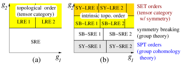
Figure 1: (Color online) (a) The possible gapped phases for a class of Hamiltonians $H(g_{1},g_{2})$ without any symmetry. (b) The possible gapped phases for the class of Hamiltonians $H_{\text{symm}}(g_{1},g_{2})$ with a symmetry. The yellow regions in (a) and (b) represent the phases with long range entanglement. Each phase is labeled by its entanglement properties and symmetry breaking properties. SRE stands for short range entanglement, LRE for long range entanglement, SB for symmetry breaking, SY for no symmetry breaking. SB-SRE phases are the Landau symmetry breaking phases. The SY-SRE phases are the SPT phases. The SY-LRE phases are the SET phases.

SRE states are states that can be transformed into direct product states via LU transformations. All SRE states can be transformed into each other via LU transformations, and thus all SRE states belong to the same phase (see Fig. 1a). LRE states are states that cannot be transformed into direct product states via LU transformations. There are LRE states that cannot be connected to each other through LU transformations. Those LRE states represent different quantum phases, which are nothing but the topologically ordered phases. Chiral spin liquids,Kalmeyer and Laughlin (1987); Wen et al. (1989) fractional quantum Hall statesTsui et al. (1982); Laughlin (1983), $Z_{2}$ spin liquids,Read and Sachdev (1991); Wen (1991a); Moessner and Sondhi (2001) non-Abelian fractional quantum Hall states,Moore and Read (1991); Wen (1991b); Willett et al. (1987); Radu et al. (2008) etc are examples of topologically ordered phases.

Topological order and long-range entanglement, as truly new phenomena, even require new mathematical language to describe them. It appears that tensor category theoryFreedman et al. (2004); Levin and Wen (2005); Chen et al. (2010); Gu et al. (2010) and simple current algebraMoore and Read (1991); Lu et al. (2010) may be part of the new mathematical language. Using the new language, we have developed a systematic and quantitative theory for non-chiral topological orders in 2D interacting boson and fermion systems.Levin and Wen (2005); Chen et al. (2010); Gu et al. (2010) Also for chiral 2D topological orders with only Abelian statistics, we find that we can use integer $K$-matrices to classify them.Blok and Wen (1990); Read (1990); Fröhlich and Kerler (1991); Wen and Zee (1992); Belov and Moore (2005); Kapustin and Saulina (2011)

I.2 Short-range entangled states with symmetry

For gapped quantum systems with symmetry, the structure of phase diagram is much richer (see Fig. 1b). Even SRE states now can belong to different phases, which include the well known Landau symmetry breaking states. But even SRE states that do not break any symmetry can belong to different phases, despite they all have trivial topological order and vanishing symmetry breaking order parameters. The 1D Haldane phase for spin-1 chainHaldane (1983); Affleck et al. (1988); Gu and Wen (2009); Pollmann et al. (2012) and topological insulatorsKane and Mele (2005a); Bernevig and Zhang (2006); Kane and Mele (2005b); Moore and Balents (2007); Fu et al. (2007); Qi et al. (2008) are non-trivial examples of SRE phases that do not break any symmetry. We will refer this kind of phases as symmetry-protected trivial (SPT) phases or symmetry-protected topological (SPT) phases.Gu and Wen (2009); Pollmann et al. (2012) Note that the SPT phases have no long range entanglement and have trivial topological orders.

It turns out that there is no gapped bosonic LRE state in 1+1D (i.e. topological order does not exist in 1+1D).Verstraete et al. (2005) So all 1D gapped bosonic states are either symmetry breaking states or SPT states. This realization led to a complete classification of all 1+1D gapped bosonic quantum phases.Chen et al. (2011a); Schuch et al. (2011); Chen et al. (2011b)

In LABEL:CLW1141,CGL1172,CGL1204, the classification of 1+1D SPT phases is generalized to any dimensions:

For gapped bosonic systems in $d$ space-time dimensions with an on-site symmetry group $SG$, the SPT phases that do not break the symmetry are described by the elements in ${\cal H}^{d}[SG,\mathbb{R}/\mathbb{Z}]$ – the group cohomology class of $SG$.

Such a systematic understanding of SPT states was obtained by thinking those states as “trivial” short range entangled states rather then topologically ordered states. The group cohomology theory predicted several new bosonic topological insulators and bosonic topological superconductors, as well as many other new quantum phases with different symmetries and in different dimensions. This led to an intense research activity on SPT states.Levin and Stern (2009); Lu and Vishwanath (2012); Liu and Wen (2013); Chen and Wen (2012); Hung and Wen (2012); Hung and Wan (2012); Vishwanath and Senthil (2013); Xu (2013); Lu and Lee (2012a); Hung and Wen (2013); Lu and Lee (2012b); Ye and Wen (2013a); Oon et al. (2012); Xu and Senthil (2013); Wang and Senthil (2013); Burnell et al. (2013); Cheng and Gu (2013); Chen et al. (2013b, c); Ye and Wen (2013b); Metlitski et al. (2013); Gu and Levin (2013); Lu and Vishwanath (2013)

What are the “topological order parameters” or more precisely SPT invariants that can be used to characterize SPT states? One way to characterize SPT states is to gauge the on-site symmetry and use the introduced gauge field as an effective probe for the SPT order.Levin and Gu (2012) This will be the main theme of this paper. After we integrate out the matter fields, a non-trivial SPT phase will leads to a non-trivial quantized gauge topological term.Hung and Wen (2012) So one can use the induced gauge topological terms, as the “topological order parameters” or SPT invariants, to characterize the SPT phases. It turns out that the quantized gauge topological terms for gauge group $SG$ is also classified by the same group cohomology class ${\cal H}^{d}[SG,\mathbb{R}/\mathbb{Z}]$. Thus the gauge-probe will allow us to fully characterize the SPT phases. We will use the structure of ${\cal H}^{d}[SG,\mathbb{R}/\mathbb{Z}]$ as a guide to help us to construct the SPT invariants for the SPT states. Another general way to obtain SPT invariants is to study boundary states, which is effective for both topological orderWen (1992); Wang and Wen (2012); Levin (2013) and SPT order.Chen et al. (2011a); Vishwanath and Senthil (2013)

We like to point out that the gauge approach can also be applied to fermion systems.

We can use the elements in ${\cal H}^{d}[G_{f},\mathbb{R}/\mathbb{Z}]$ to characterize fermionic SPT statesGu and Wen (2012) in $d$ space-time dimensions with a full symmetry group $G_{f}$ (see section III.4.1).

However, it is not clear if every element in ${\cal H}^{d}[G_{f},\mathbb{R}/\mathbb{Z}]$ can be realized by fermion systems or not. It is also possible that two different elements in ${\cal H}^{d}[G_{f},\mathbb{R}/\mathbb{Z}]$ may correspond to the same fermionic SPT state. Despite the incomplete result, we can still use ${\cal H}^{d}[G_{f},\mathbb{R}/\mathbb{Z}]$ to guide us to construct the SPT invariants for fermionic SPT states.

I.3 Long-range entangled states with symmetry

For gapped LRE states with symmetry, the possible quantum phases should be even richer than SRE states. We may call those phases Symmetry Enriched Topological (SET) phases. At moment, we do not have a classification or a systematic description of SET phases. But we have some partial results.

Projective symmetry group (PSG) was introduced in 2002 to study the SET phases.Wen (2002, 2003); Wang and Vishwanath (2006) The PSG describes how the quantum numbers of the symmetry group $SG$ get fractionalized on the gauge excitations.Wen (2003) When the gauge group $GG$ is Abelian, the PSG description of the SET phases can be be expressed in terms of group cohomology: The different SET states with symmetry $SG$ and gauge group $GG$ can be (partially) described by a subset of ${\cal H}^{2}(SG,GG)$.Essin and Hermele (2013)

One class of SET states in $d$ space-time dimensions with global symmetry $SG$ are described by weak-coupling gauge theories with gauge group $GG$ and quantized topological terms (assuming the weak-coupling gauge theories are gapped, that can happen when the space-time dimension $d=3$ or when $d>3$ and the gauge group $GG$ is finite). Those SET states (i.e. the quantized topological terms) are described by the elements in ${\cal H}^{d}(PSG,\mathbb{R}/\mathbb{Z})$,Mesaros and Ran (2013); Hung and Wen (2013) where the group $PSG$ is an extension of $SG$ by $GG$: $SG=PSG/GG$. Or in other words, we have a short exact sequence

$$1\to GG\to PSG\to SG\to 1.$$ (1)

We will denote $PSG$ as $PSG=GG\rightthreetimes SG$. Many examples of the SET states can be found in LABEL:W0213,KLW0834,KW0906,LS0903,YFQ1070.

Although we have a systematic understanding of SPT phases and some of the SET phases in term of ${\cal H}^{d}(SG,\mathbb{R}/\mathbb{Z})$ and ${\cal H}^{d}(PSG,\mathbb{R}/\mathbb{Z})$, however, those constructions do not tell us to how to experimentally or numerically measure the elements in ${\cal H}^{d}(SG,\mathbb{R}/\mathbb{Z})$ or ${\cal H}^{d}(PSG,\mathbb{R}/\mathbb{Z})$ that label the different SPT or SET phases. We do not know, even given an exact ground state wave function, how to determine which SPT or SET phase the ground state belongs to.

In this paper, we will address this important question. We will find physical ways to the detect different SPT/SET phases and to measure the elements in ${\cal H}^{d}(SG,\mathbb{R}/\mathbb{Z})$ or ${\cal H}^{d}(PSG,\mathbb{R}/\mathbb{Z})$. This is achieved by gauging the symmetry group $SG$ (i.e. coupling the $SG$ quantum numbers to a $SG$ gauge potential $A^{\text{SG}}$). Note that $A^{\text{SG}}$ is treated as a non-fluctuating probe field. By study the topological response of the system to various $SG$ gauge configurations, we can measure the elements in ${\cal H}^{d}(SG,\mathbb{R}/\mathbb{Z})$ or ${\cal H}^{d}(PSG,\mathbb{R}/\mathbb{Z})$. Those topological response are the measurable SPT invariants (or “topological order parameters”) that characterize the SPT/SET phases. Tables 1 and 2, and the SPT invariant statements in the paper, describe the many constructed SPT invariants, and represent the main results of the paper.

II SPT invariants of SPT states: a general discussion

Because of the duality relation between the SPT states and the SET states described by weak-coupling gauge theoriesLevin and Gu (2012); Mesaros and Ran (2013); Hung and Wen (2013) (see appendix E), in this paper, we will mainly discuss the physical properties and the SPT invariants of the SPT state. The physical properties and the topological invariants of the SET states can be obtained from the physical properties and the SPT invariants of corresponding SPT states via the duality relation.

II.1 Gauge the symmetry and twist the space

Let us consider a system with symmetry group $G$ in $d$ space-time dimensions. The ground state of the system is a SPT state described by an element $\nu_{d}$ in ${\cal H}^{d}(G,\mathbb{R}/Z)$. But how to physically measure $\nu_{d}$? Following the idea of LABEL:LG1220, we will propose to measure $\nu_{d}$ by “gauging” the symmetry $G$, i.e. by introducing a $G$ gauge potential $A_{\mu}(x^{i})$ to couple to the quantum numbers of $G$. The $G$ gauge potential $A_{\mu}$ is a fixed probe field, not a dynamical field. We like to consider how the system responds to various $G$ gauge configurations described by $A_{\mu}$. We will show that the topological responses allow us to fully measure the cocycle $\nu_{d}$ that characterizes the SPT phase, at least for the many cases considered. Those topological responses are the SPT invariants that we are looking for.

There are several topological responses that we can use to construct SPT invariants:

1. We set up a time independent $G$ gauge configuration $A_{\mu}(x^{i})$. If the gauge configuration is invariant under a subgroup $GG$ of $G$: $A_{\mu}(x^{i})=h^{-1}A_{\mu}(x^{i})h$, $h\in GG$ , then we can study the conserved $GG$ quantum number of the ground state under such gauge configuration. Some times, the ground states may be degenerate which form a higher dimensional representation of $GG$.

   In particular, the time independent $G$ gauge configuration may be chosen to be a monopole-like or other soliton-like gauge configuration. The quantum number of the unbroken symmetry carried by those defects can be SPT invariants of the SPT states.

   We can also remove $n$ identical regions $D(i)$, $i=1,\cdots,n$, from the space $M_{d-1}$ to get a $(d-1)$-dimensional manifold $M^{\prime}_{d-1}$ with $n$ “holes”. Then we consider a flat $G$ gauge configuration $A_{\mu}(x^{i})$ on $M^{\prime}_{d-1}$ such that the gauge fields near the boundary of those “holes”, $\partial D(i)$, are identical. We then measure the conserved $GG$ quantum number on the ground state for such $G$ gauge configuration. We will see that the $GG$ quantum number may not be multiples of $n$, indicating a non-trivial SPT phases.

2. We may choose the space to have a form $M_{k}\times M_{d-k-1}$ where $M_{k}$ is a closed $k$-dimensional manifold or a closed $k$-dimensional manifold with $n$ identical holes. $M_{d-k-1}$ is a closed $(d-k-1)$-dimensional manifold. We then put a $G$ gauge configuration $A_{\mu}(x^{i})$ on $M_{k}$, or a flat $G$ gauge configuration on $M_{k}$ if $M_{k}$ has $n$ holes. In the large $M_{d-k-1}$ limit, our system can be viewed as a system in $(d-k-1)$-dimensional space with a symmetry $GG$, where $GG\subset G$ is formed by the symmetry transformations that leave the $G$ gauge configuration invariant. The ground state of the system is a SPT state characterized by cocycles in ${\cal H}^{d-k}(GG,\mathbb{R}/\mathbb{Z})$. The mapping from the gauge configurations on $M_{k}$ to ${\cal H}^{d-k}(GG,\mathbb{R}/\mathbb{Z})$ is our SPT invariant.

3. We can have a family of $G$ gauge configurations $A_{\mu}(x^{i})$ that have the same energy. As we go around a loop in such a family of $G$ gauge configurations, the corresponding ground states will generate a geometric phase (or non-Abelian geometric phases if the ground states are degenerate). Sometimes, the (non-Abelian) geometric phases are also SPT invariants which allow us to probe and measure the cocycles. One such type of the SPT invariants is the statistics of the $G$ gauge vortices in 2+1D or monopoles in 3+1D.

4. The above topological responses can be measured in a Hamiltonian formulation of the system. In the imaginary-time path-integral formulation of the system where the space-time manifold $M_{d}$ can have an arbitrary topology, we can have a most general construction of SPT invariants. We simply put a nearly-flat $G$ gauge configuration on a closed space-time manifold $M_{d}$ and evaluate the path integral. We will obtain a partition function $Z(M_{d},A_{\mu})$ which is a function of the space-time topology $M_{d}$ and the nearly-flat gauge configuration $A_{\mu}$. In the limit of the large volume $V=\lambda^{d}V_{0}$ of the space-time (i.e. $\lambda\to\infty$), $Z(M_{d},A_{\mu})$ has a form (assuming we only scale the space-time volume without any change in shape)

   $$Z(M_{d},A_{\mu})=\hskip 1.0pt\mathrm{e}^{-\sum_{n=1}^{d}f_{n}\lambda^{n}}Z_{\text{top}}(M_{d},A_{\mu}),$$ (2)

   where $Z_{\text{top}}(M_{d},A_{\mu})$ is independent of the scaling factor $\lambda$. $Z_{\text{top}}(M_{d},A_{\mu})$ is a SPT invariant that allows us to fully measure the elements in ${\cal H}^{d}(G,\mathbb{R}/Z)$ that describe the SPT phases.Dijkgraaf and Witten (1990); Hung and Wen (2012); Hu et al. (2013) In fact, $Z_{\text{top}}(M_{d},A_{\mu})$ is the partition function for the pure topological term $W^{\text{gauge}}_{\text{top}}(g,A)$ in eqn. (182).

   We like to point out that if $Z_{\text{top}}(M_{d},A_{\mu})$ contain a Chern-Simons term (i.e. $Z_{\text{top}}(M_{d},A_{\mu})=\hskip 1.0pt\mathrm{e}^{\hskip 1.0pt\mathrm{i}\hskip 1.0pt\int{\cal L}_{CS}}$), then it describes an SPT phase that is labeled by an element in the free part of ${\cal H}^{d}(G,\mathbb{R}/Z)$. If $Z_{\text{top}}(M_{d},A_{\mu})$ is a topological term whose value is independent of any small perturbations of $A_{\mu}$, then it describes an SPT phase that is labeled by an element in the torsion part of ${\cal H}^{d}(G,\mathbb{R}/Z)$.Hung and Wen (2012)

II.2 Cup-product, Künneth formula, and SPT invariants

The cohomology class ${\cal H}^{d}(G,\mathbb{R}/\mathbb{Z})\cong{\cal H}^{d+1}(G,\mathbb{Z})$ is not only an Abelian group. The direct sum of ${\cal H}^{d+1}(G,\mathbb{Z})$, ${\cal H}^{*}(G,\mathbb{Z})=\oplus_{d}{\cal H}^{d}(G,\mathbb{Z})$, also has a cup-product that makes ${\cal H}^{*}(G,\mathbb{Z})$ into a ring:

$$\nu_{d_{1}}\cup\nu_{d_{1}} =\nu_{d_{1}+d_{2}}, \nu_{d_{1}+d_{2}} \in{\cal H}^{d_{1}+d_{2}}(G,\mathbb{Z}),$$

$$\nu_{d_{1}} \in{\cal H}^{d_{1}}(G,\mathbb{Z}), \nu_{d_{1}} \in{\cal H}^{d_{1}}(G,\mathbb{Z}).$$ (3)

We also have the Künneth formula

$${\cal H}^{d} (GG\times SG,\mathbb{R}/\mathbb{Z})=\oplus_{k=0}^{d}{\cal H}^{k}[SG,{\cal H}^{d-k}(GG,\mathbb{R}/\mathbb{Z})]$$

$$=\oplus_{k=0}^{d}{\cal H}^{k}[GG,{\cal H}^{d-k}(SG,\mathbb{R}/\mathbb{Z})]$$

$$=\left(\oplus_{k=1}^{d}{\cal H}^{k-1}(GG,\mathbb{R}/\mathbb{Z})\otimes_{\mathbb{Z}}{\cal H}^{d-k}(SG,\mathbb{R}/\mathbb{Z})\right)\oplus$$

$$\ \ \ \,\left(\oplus_{k=0}^{d}{\cal H}^{k}(GG,\mathbb{R}/\mathbb{Z})\boxtimes_{\mathbb{Z}}{\cal H}^{d-k}(SG,\mathbb{R}/\mathbb{Z})\right).$$ (4)

(see eqn. (C) and eqn. (C)). Both of the above two results relate cocycles at higher dimensions to cocycles at lower dimensions. The structures of the cup-product and Künneth formula give us some quite direct hints on how to construct SPT invariants that probe the cocycles. For example, consider a SPT state with symmetry $GG\times SG$, which is label by an element in ${\cal H}^{d}(GG\times SG,\mathbb{R}/\mathbb{Z})$. If such an element belong to ${\cal H}^{k-1}(GG,\mathbb{R}/\mathbb{Z})\otimes_{\mathbb{Z}}{\cal H}^{d-k}(SG,\mathbb{R}/\mathbb{Z})$ or ${\cal H}^{k}(GG,\mathbb{R}/\mathbb{Z})\boxtimes_{\mathbb{Z}}{\cal H}^{d-k}(SG,\mathbb{R}/\mathbb{Z})$, then we can choose the space-time to have a topology $M_{k}\times M_{d-k}$. Next we try to design a defect that couple to ${\cal H}^{k-1}(GG,\mathbb{R}/\mathbb{Z})={\cal H}^{k}(GG,\mathbb{Z})$ or ${\cal H}^{k}(GG,\mathbb{R}/\mathbb{Z})$ on $M_{k}$ and try to measure the response described by ${\cal H}^{d-k}(SG,\mathbb{R}/\mathbb{Z})$ on $M_{d-k}$. (See also SPT invariant 12 and 16.) For simple examples, see sections IV.4.1 and IV.5.2.

In this paper, we will review some known SPT invariants, such as Hall conductance and defect statistics, for some simple SPT states, such as 2+1D $U(1)\times U(1)$, $U(1)\times Z_{n}$, and $Z_{m}\times Z_{n}$ SPT states,Levin and Stern (2009); Levin and Gu (2012); Lu and Vishwanath (2012); Hung and Wen (2013); Gu and Levin (2013); Lu and Vishwanath (2013) and 3+1D $U(1)\rtimes Z_{2}^{T}$ SPT state.Metlitski et al. (2013) We will also introduce some additional SPT invariants, such as total quantum number of the identical monodromy defects that can be created on a closed space and the dimension reduction of SPT states, for those simple SPT states. We compare those SPT invariants to the structures of the cup-product and Künneth formula. This comparison helps us to understand the relation between the cup-product/Künneth-formula and the SPT invariants.

We will discuss SPT invariants in many examples of SPT states, starting from simple ones. Each example offers a little bit of new features than previous example. We hope that, through those examples, we will build some intuitions of constructing SPT invariants for general SPT states. Such an intuition and understanding, in turn, help us to construct new SPT invariants for more complicated SPT states (see SPT invariant 12 and 16). The new understanding allows us to construct SPT invariants for more general SPT states in 1+1D, 2+1D and 3+1D. The main results are summarize in Table 1.

III SPT invariants of SPT states with simple symmetry groups

III.1 Bosonic $Z_{n}$ SPT phases

III.1.1 0+1D

In $1$-dimensional space-time, the bosonic SPT states with symmetry $Z_{n}=\{g^{(k)}=\hskip 1.0pt\mathrm{e}^{2\pi k\hskip 1.0pt\mathrm{i}\hskip 1.0pt/n}|k=0,\cdots,n-1\}$ are described by the cocycles in ${\cal H}^{1}(Z_{n},\mathbb{R}/\mathbb{Z})=\mathbb{Z}_{n}$. How to measure the cocycles in ${\cal H}^{1}(Z_{n},\mathbb{R}/\mathbb{Z})$? What is the measurable SPT invariants that allow us to characterize the $Z_{n}$ SPT states?

One way to construct a SPT invariant is to gauge the $Z_{n}$ global symmetry in the action that describes that SPT state, and obtain a $Z_{n}$-gauge theory ${\cal L}(g_{i},h_{ij})$, where $h_{ij}\in Z_{n}$ is the $Z_{n}$-gauge “connection” on the link connecting vertices $i$ and $j$, and $g_{i}\in Z_{n}$ is the “matter” field that describes the SPT state (if we set $h_{ij}=1$). Due to the gauge invariance, ${\cal L}(g_{i},h_{ij})$ has a form ${\cal L}(g_{i},h_{ij})={\cal L}(g_{i}^{-1}h_{ij}g_{j})$ (see eqn. (188)).

After integral out the “matter” fields $g_{i}$, we obtain a SPT invariant which appears as a topological term in the $Z_{n}$-gauge theory $Z_{\text{top}}(M_{d},A_{\mu})=Z_{\text{top}}(M_{d},h_{ij})$. (Note that, in a $Z_{n}$ gauge theory, $h_{ij}$ is the gauge “connection” $A_{\mu}$.) The $Z_{n}$-gauge topological term can be expressed in term of cocycles $\omega_{1}(h_{ij})$:

$$Z_{\text{top}}(S_{1},A_{\mu})=\hskip 1.0pt\mathrm{e}^{\hskip 1.0pt\mathrm{i}\hskip 1.0pt2\pi\sum_{i}\omega_{1}(h_{i,i+1})},$$ (5)

where we have assumed that the space-time is a circle $S_{1}$ formed by a ring of vertices labeled by $i$.

In fact, before we integrate out that “matter” field $g_{i}$, the partition function for an ideal fixed-point SPT Lagrangian is given by (see eqn. (188))

$$Z(S_{1},A_{\mu})=\sum_{\{g_{i}\}}\hskip 1.0pt\mathrm{e}^{\hskip 1.0pt\mathrm{i}\hskip 1.0pt2\pi\sum_{i}\omega_{1}(g_{i}^{-1}h_{i,i+1}g_{i+1})},$$ (6)

where $\sum_{\{g_{i}\}}$ sums over all the $g_{i}$ configurations on $S_{1}$. Since $\hskip 1.0pt\mathrm{e}^{\hskip 1.0pt\mathrm{i}\hskip 1.0pt2\pi\sum_{i}\omega_{1}(g_{i}^{-1}h_{i,i+1}g_{i+1})}$ is independent of $\{g_{i}\}$, we can integrate out $g_{i}$ easily and obtain eqn. (5).

A $Z_{n}$-gauge configuration on $S_{1}$ is given by $Z_{n}$ group elements $h_{i,i+1}$ on each link $(i,i+1)$. We may view the cocycle $\omega_{1}$ as a “discrete differential form” and use the differential form notion to express the above topological action amplitude (which is also a $Z_{n}$-gauge topological term)

$$Z_{\text{top}}(S_{1},A_{\mu})=\hskip 1.0pt\mathrm{e}^{\hskip 1.0pt\mathrm{i}\hskip 1.0pt2\pi\int_{S_{1}}\omega_{1}(h_{i,i+1})}.$$ (7)

For more details on such a notation, see appendix A.4. The cocycle condition (see appendix A) ensures that

$$Z_{\text{top}}(S_{1},A_{\mu})=\hskip 1.0pt\mathrm{e}^{\hskip 1.0pt\mathrm{i}\hskip 1.0pt2\pi\int_{S_{1}}\omega_{1}(h_{i,i+1})}=1$$ (8)

if $h_{i,i+1}=g^{i+1}g^{-1}_{i}$ is a pure $Z_{n}$-gauge.

The cocycles in ${\cal H}^{1}(Z_{n},\mathbb{R}/\mathbb{Z})=\mathbb{Z}_{n}$ are labeled by $m=0,\cdots,n-1$ with $m=0$ corresponding to the trivial cocycle. The $m^{th}$ cocycle is given by

$$\omega_{1}(g^{(k)})=\text{mod}(mk/n,1)$$ (9)

We note that the above cocycle $\omega_{1}(h_{i,i+1})$ is a torsion element in ${\cal H}^{1}(Z_{n},\mathbb{R}/\mathbb{Z})$. It gives rise to a quantized topological term $Z_{\text{top}}(S_{1},A_{\mu})$:

$$\hskip 1.0pt\mathrm{e}^{\hskip 1.0pt\mathrm{i}\hskip 1.0pt2\pi\int_{S_{1}}\omega_{1}(h_{i,i+1})} =\hskip 1.0pt\mathrm{e}^{2\pi mk\hskip 1.0pt\mathrm{i}\hskip 1.0pt/n},\ \text{ if }\prod_{i}h_{i,i+1}=g^{(k)}.$$ (10)

Such a partition function is a SPT invariant. Its non-trivial dependence on the total $Z_{n}$ flux through the circle, $g^{(k)}=\prod_{i}h_{i,i+1}$, implies that the SPT state is non-trivial.

The above partition function also implies that the ground state of the system carries a $Z_{n}$ quantum number $m$. Thus the non-trivial $Z_{n}$ quantum number of the ground state $m\neq 0$ also measure the non-trivial cocycle in ${\cal H}^{1}(Z_{n},\mathbb{R}/\mathbb{Z})$.

III.1.2 Monodromy defect

In $3$-dimensional space-time, the bosonic $Z_{n}$ SPT states are described by the cocycles in ${\cal H}^{3}(Z_{n},\mathbb{R}/\mathbb{Z})=\mathbb{Z}_{n}$. To find the SPT invariants for such a case, let us introduce the notion of monodromy defect.Levin and Gu (2012)

Let us assume that the 2D lattice Hamiltonian for a SPT state with symmetry $G$ has a form (see Fig. 2)

$$H=\sum_{(ijk)}H_{ijk},$$ (11)

where $\sum_{(ijk)}$ sums over all the triangles in Fig. 2 and $H_{ijk}$ acts on the states on site-$i$, site-$j$, and site-$k$: $|g_{i}g_{j}g_{k}\rangle$. (Note that the states on site-$i$ are labeled by $g_{i}\in G$.) $H$ and $H_{ijk}$ are invariant under the global $G$ transformations.

Let us perform a $G$ transformation only in the shaded region in Fig. 2. Such a transformation will change $H$ to $H^{\prime}$. However, only the Hamiltonian terms on the triangles $(ijk)$ across the boundary are changed from $H_{ijk}$ to $H^{\prime}_{ijk}$. Since the $G$ transformation is an unitary transformation, $H$ and $H^{\prime}$ have the same energy spectrum. In other words the boundary in Fig. 2 (described by $H^{\prime}_{ijk}$’s) do not cost any energy.

Now let us consider a Hamiltonian on a lattice with a “cut” (see Fig. 3)

$$\tilde{H}={\sum_{(ijk)}}^{\prime}H_{ijk}+{\sum_{(ijk)}}^{\text{cut}}H^{\prime}_{ijk}$$ (12)

where $\sum^{\prime}_{(ijk)}$ sums over the triangles not on the cut and $\sum^{\text{cut}}_{(ijk)}$ sums over the triangles that are divided into disconnected pieces by the cut. The triangles at the ends of the cut have no Hamiltonian terms. We note that the cut carries no energy. Only the ends of cut cost energies. Thus we say that the cut corresponds to two monodromy defects. The Hamiltonian $\tilde{H}$ defines the two monodromy defects.

We also like to point out that the above procedure to obtain $\tilde{H}$ is actually the “gauging” of the $G$ symmetry. $\tilde{H}$ is a gauged Hamiltonian that contain a $G$ vortex-antivortex pair at the ends of the cut.

To summarize, a system with on-site symmetry $G$ can have many monodromy defects, labeled by the group elements that generate the twist along the cut. When $G$ is singly generated, we will call the monodromy defect generated by the natural generator of $G$ as elementary monodromy defect. In this case, other monodromy defects can be viewed a bound states of several elementary monodromy defects. In the rest of this paper, we will only consider the elementary monodromy defects.

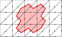
Figure 2: (Color online) A 2D lattice on a torus. A $Z_{n}$ transformation is performed on the sites in the shaded region. The $Z_{n}$ transformation changes the Hamiltonian term on the triangle $(ijk)$ across the boundary from $H_{ijk}$ to $H^{\prime}_{ijk}$.

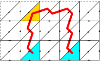
Figure 3: (Color online) A $Z_{2}$-gauge configuration with two identical $Z_{2}$ vertices (or two monodromy defects) on a torus. Such a $Z_{2}$-gauge configuration has $U^{\text{bulk}}_{-1}=-1$ (each yellow triangle contributes a factor $-1$). Thus $U^{\text{bulk}}_{g}$ forms a 1D representation of $Z_{2}$ with a $Z_{2}$-charge 1.

III.1.3 2+1D: total $Z_{n}$-charge of $n$ identical monodromy defects

The SPT invariant to detect the cocycle in ${\cal H}^{3}(Z_{n},\mathbb{R}/\mathbb{Z})$ is the $Z_{n}$ quantum number of $n$ identical monodromy defects created by the twist $g^{(1)}\in Z_{n}$ (see Fig. 3). Note that the monodromy defects created by $g^{(1)}$ are the elementary monodromy defects. Other elementary monodromy defects can be viewed as bound states of the elementary monodromy defects. Also note that the monodromy defects or the $Z_{n}$-vortices are identical which correspond to the same kind of $\begin{matrix}\includegraphics[height=18.06749pt]{tri1}\end{matrix}$ triangles.

Since ${\cal H}^{3}(Z_{n},\mathbb{R}/\mathbb{Z})=\mathbb{Z}_{n}$, the 2+1D $Z_{n}$ SPT states are labeled by $m=0,\cdots,n-1$, with the corresponding 3-cocycle given by

$$\omega_{3}(g^{(k_{1})},g^{(k_{2})},g^{(k_{3})}) =\hskip 1.0pt\mathrm{e}^{m\frac{2\pi\hskip 1.0pt\mathrm{i}\hskip 1.0pt}{n^{2}}k_{1}(k_{2}+k_{3}-[k_{2}+k_{3}]_{n})},$$

$$g^{(k)} =\hskip 1.0pt\mathrm{e}^{\frac{2\pi k\hskip 1.0pt\mathrm{i}\hskip 1.0pt}{n}},$$ (13)

where $[k]_{n}$ is a short-hand notation for

$$[k]_{n}\equiv\text{mod}(k,n).$$ (14)

In appendix F.2, we show that

SPT invariant 1:

$n$ identical monodromy defects generated by $g^{(1)}$ twist in 2+1D $Z_{n}$ SPT states on a torus always carry a total $Z_{n}$-charge $2m$, if the $Z_{n}$ SPT states are described by the $m^{th}$ cocycle in ${\cal H}^{3}(Z_{n},\mathbb{R}/\mathbb{Z})$.

When $n=$odd, we find that the total $Z_{n}$-charge of $n$ identical monodromy defects allows us to completely characterize the 2+1D $Z_{n}$ SPT states. However, when $n=$even, the total $Z_{n}$-charge of $n$ identical monodromy defects only allows us to distinguish $n/2$ different $Z_{n}$ SPT states. The $m$ and $m+\frac{n}{2}$ $Z_{n}$ SPT states give rise to the same total $Z_{n}$ charge, and cannot be distinguished this way.

We like to point out that when constructing the above SPT invariant, we have assumed that the system has an additional translation symmetry although the existence of the $Z_{n}$ SPT states do not require the translation symmetry. We use the translation symmetry to make identical monodromy defects, which allow us to construct the above SPT invariant.

III.1.4 2+1D: the statistics of the monodromy defects

To construct new SPT invariant that can distinguish $m$ and $m+\frac{n}{2}$ $Z_{n}$ SPT states, we will consider the statistics of the (elementary) monodromy defects.Levin and Gu (2012) To compute the statistics of the monodromy defects we will use the duality relation between the $Z_{n}$ SPT states and the twisted $Z_{n}$ gauge theory discovered by Levin and Gu.Levin and Gu (2012) The (twisted) $Z_{n}$ gauge theory can be studied using $U(1)\times U(1)$ Chern-Simons theory.Kou et al. (2008); Levin and Stern (2009); Lu and Vishwanath (2012); Hung and Wen (2013)

The $Z_{n}$ SPT states are described by ${\cal H}^{3}(Z_{n},\mathbb{R}/\mathbb{Z})=\{m|m=0,\cdots,n-1\}$. Thus, the $Z_{n}$ integer $m$ labels different 2+1D $Z_{n}$ SPT states. The dual gauge theory description of the $Z_{n}$ SPT state (labeled by $m$) is given by

$${\cal L}+W_{\text{top}}=\frac{1}{4\pi}K_{IJ}a_{I\mu}\partial_{\nu}a_{J\lambda}+...$$ (15)

with

$$K=\begin{pmatrix}-2m&n\\ n&0\\ \end{pmatrix}.$$ (16)

The $K$-matrix with $K_{11}=-2m$ correspond to the 3-cocycle in eqn. (III.1.3).Hung and Wen (2013) Note that, here, $a_{I\mu}$ are dynamical gauge fields whose charges are quantized as integers. They are not the fixed probe gauge fields which are denoted by capital letter $A_{\mu}$. Two $K$-matrices $K_{1}$ and $K_{2}$ are equivalent $K_{1}\sim K_{2}$ (i.e. give rise to the same theory) if $K_{1}=U^{T}K_{2}U$ for an integer matrix with det$(U)=\pm 1$. We find that $K(m)\sim K(m+n)$. Thus only $m=0,\cdots,n-1$ give rise to nonequivalent $K$-matrices.

A particle carrying $l_{I}$ $a^{I}_{\mu}$-charge will have a statistics

$$\theta_{l}=\pi l_{I}(K^{-1})^{IJ}l_{J}.$$ (17)

A particle carrying $l_{I}$ $a^{I}_{\mu}$-charge will have a mutual statistics with a particle carrying $\tilde{l}_{I}$ $a^{I}_{\mu}$-charge:

$$\theta_{l,\tilde{l}}=2\pi l_{I}(K^{-1})^{IJ}\tilde{l}_{J}.$$ (18)

A particle with a unit of $Z_{n}$-charge is described by a particle with a unit $a^{1}_{\mu}$-charge. Using

$$K^{-1}=\frac{1}{n^{2}}\begin{pmatrix}0&n\\ n&2m\\ \end{pmatrix},$$ (19)

we find that the $Z_{n}$-charge (the unit $a^{1}_{\mu}$-charge) are always bosonic.

The $Z_{n}$ monodromy defect in the original theory corresponds to $2\pi/n$-flux in $a^{1}_{\mu}$, since the unit $a^{1}_{\mu}$-charge corresponds to the $Z_{n}$-charge in the original theory. We note that a particle carry $l_{I}$ $a^{I}_{\mu}$-charge created a $l_{2}\pi$ flux in $a^{1}_{\mu}$. So a unit $a^{2}_{\mu}$-charge always represent a $Z_{n}$ monodromy defect. But such a $Z_{n}$ monodromy defect may not be a pure $Z_{n}$ monodromy defect. It may carry some additional $Z_{n}$-charges.

Since the $Z_{n}$ monodromy defect correspond to $2\pi/n$-flux in $a^{1}_{\mu}$, by itself, a single monodromy defect is not an allowed excitation. However, $n$ identical $Z_{n}$ monodromy defects (i.e. $n$ particles that each carries a unit $a^{2}_{\mu}$-charge) correspond to $2\pi$-flux in $a^{1}_{\mu}$ which is an allowed excitation. Then, what is the total $Z_{n}$ charge of $n$ identical $Z_{n}$ monodromy defects (i.e. $n$ units of $a^{2}_{\mu}$-charges)? We note that $n$ units of $a^{2}_{\mu}$-charges can be viewed as a bound state of a particle with $(l_{1},l_{2})=(-2m,n)$ $a^{I}_{\mu}$-charges and a particle with $(l_{1},l_{2})=(2m,0)$ $a^{I}_{\mu}$-charges. The particle with $(l_{1},l_{2})=(2m,n)$ $a^{I}_{\mu}$-charges is a trivial excitation that carry zero $Z_{n}$ charge, since $(l_{1},l_{2})=(-2m,n)$ is a row of the $K$-matrix. The particle with $(l_{1},l_{2})=(2m,0)$ $a^{I}_{\mu}$-charges carries $2m$ $Z_{n}$ charges. Thus, $n$ identical $Z_{n}$ monodromy defects (described by $n$ particles that each carries a unit $a^{2}_{\mu}$-charge) have $2m$ total $Z_{n}$ charges, which agrees with the result obtained the in last section.

A particle that carries a unit $a^{2}_{\mu}$-charge is only one way to realize the $Z_{n}$ monodromy defect. A generic $Z_{n}$ monodromy defect that may carry a different $Z_{n}$-charge corresponds to $\bm{l}^{M}=(l^{M}_{1},1)$ $a^{I}_{\mu}$-charge. The statistics of such generic $Z_{n}$ monodromy defect is

$$\theta_{M}=\pi(\bm{l}^{M})^{T}K^{-1}\bm{l}^{M}=2\pi(\frac{l^{M}_{1}}{n}+\frac{m}{n^{2}}).$$ (20)

We find that

SPT invariant 2:

the statistical angle $\theta_{M}$ of an elementary monodromy defect is a SPT invariant that allows us to fully characterize the 2+1D bosonic $Z_{n}$ SPT states.Levin and Gu (2012) In particular mod$(\frac{\theta_{M}}{2\pi},\frac{1}{n})=\frac{m}{n^{2}}$ where $m\in{\cal H}^{3}(Z_{n},\mathbb{R}/\mathbb{Z})=\mathbb{Z}_{n}$ labels the different $Z_{n}$ SPT states.

We note that such a SPT invariant can full detect the 3-cocycles in ${\cal H}^{3}(Z_{n},\mathbb{R}/\mathbb{Z})$.

III.1.5 $Z_{n}$-gauge topological term in 2+1D

Just like the 0+1D case, we can also construct a SPT invariant and probe the 3-cocycles in ${\cal H}^{3}(Z_{n},\mathbb{R}/\mathbb{Z})$ by gauging the global $Z_{n}$ symmetry. After integrating out the matter fields, we obtain a $Z_{n}$-gauge topological term. Such a $Z_{n}$-gauge topological term correspond to a 3-cocycle $\omega_{3}$ in ${\cal H}^{3}(Z_{n},\mathbb{R}/\mathbb{Z})$ which describes the $Z_{n}$ SPT states. In fact, the $Z_{n}$-gauge topological term can be directly expressed in terms of the 3-cocycle $\omega_{3}(h_{ij})$ (using the differential form notation in appendix A.4):

$$\hskip 1.0pt\mathrm{e}^{\hskip 1.0pt\mathrm{i}\hskip 1.0pt2\pi\int_{M_{3}}\omega_{3}(h_{ij})},$$ (21)

where $M_{3}$ is the 3-dimensional space-time and $h_{ij}$ the $Z_{n}$-gauge “connection” in the link $ij$. Such a $Z_{n}$-gauge topological term is a generalization of the Chern-Simons term to a discrete group $Z_{n}$.

III.1.6 4+1D

We can also generalize the above construction to 5-dimensional space-time where $Z_{n}$ SPT states are described by ${\cal H}^{5}(Z_{n},\mathbb{R}/\mathbb{Z})=\mathbb{Z}_{n}$. We choose the 4+1D space-time to have a topology $M_{2}\times M_{3}$ where $M_{3}$ and $M_{2}$ are two closed 2+1D and 2D manifolds. We then create $n$ identical $Z_{n}$ monodromy defects on $M_{2}$. In the large $M_{3}$ limit, we may view our 4+1D $Z_{n}$ SPT state on space-time $M_{3}\times M_{2}$ as a 2+1D $Z_{n}$ SPT state on $M_{3}$ which is described by ${\cal H}^{3}(Z_{n},\mathbb{R}/\mathbb{Z})$. We have

SPT invariant 3:

in a 4+1D $Z_{n}$ SPT state labeled by $m\in{\cal H}^{5}(Z_{n},\mathbb{R}/\mathbb{Z})=\mathbb{Z}_{n}$ on space-time $M_{3}\times M_{2}$, $n$ identical $Z_{n}$-vortices (i.e. $Z_{n}$-monodromy defects) on $M_{2}$, induce a 2+1D $Z_{n}$ SPT state labeled by $3m\in{\cal H}^{3}(Z_{n},\mathbb{R}/\mathbb{Z})$ on $M_{3}$ in the small $M_{2}$ limit.

We will show the above result when we discuss the $U(1)$ SPT states in 4+1D (see section III.2.3).

In the section III.1.3, we have discussed how to detect the cocycles in ${\cal H}^{3}(Z_{n},\mathbb{R}/\mathbb{Z})$, by creating $n$ identical $Z_{n}$ monodromy defects on $M_{2}$, and then measure the $Z_{n}$-charge of the ground state. So the cocycles in ${\cal H}^{5}(Z_{n},\mathbb{R}/\mathbb{Z})$ can be measured by creating $n$ identical $Z_{n}$-monodromy defects on $M_{2}$ and $n$ identical $Z_{n}$-monodromy defects on $M_{2}^{\prime}$. Then we measure the $Z_{n}$-charge of the corresponding ground state.

The above construction of $Z_{n}$ SPT invariant is motivated by the following mathematical result. First ${\cal H}^{2k+1}(Z_{n},\mathbb{R}/\mathbb{Z})\simeq{\cal H}^{2k+2}(Z_{n},\mathbb{Z})$. The generating cocycle $c_{2k+2}$ in ${\cal H}^{2k+2}(Z_{n},\mathbb{Z})$ can be expressed as a wedge product $c_{2k+2}=c_{2}\wedge c_{2}\wedge\cdots\wedge c_{2}$ where $c_{2}$ is the generating cocycle in ${\cal H}^{2}(Z_{n},\mathbb{Z})$. Since ${\cal H}^{2}(Z_{n},\mathbb{Z})\simeq{\cal H}^{1}(Z_{n},\mathbb{R}/\mathbb{Z})$, we can replace one of $c_{2}$ in $c_{2k+2}=c_{2}\wedge c_{2}\wedge\cdots\wedge c_{2}$ by $\theta_{1}$ in ${\cal H}^{1}(Z_{n},\mathbb{R}/\mathbb{Z})$, and write $c_{2k+2}=\theta_{1}\wedge c_{2}\wedge\cdots\wedge c_{2}$. Note that $c_{2}\wedge\cdots\wedge c_{2}$ describes the topological gauge configuration on $2k$ dimensional space, while $\theta_{1}$ describes the 1D representation of $Z_{n}$. This motivates us to use a $Z_{n}$ gauge configuration on $2k$ dimensional space to generate a non-trivial $Z_{n}$-charge in the ground state. In the next section, we use the similar idea to construct the SPT invariant for bosonic $U(1)$ SPT states.

III.2 Bosonic $U(1)$ SPT phases

III.2.1 0+1D

In $1$-dimensional space-time, the bosonic SPT states with symmetry $U(1)=\{\hskip 1.0pt\mathrm{e}^{\hskip 1.0pt\mathrm{i}\hskip 1.0pt\theta}\}$ are described by the cocycles in ${\cal H}^{1}[U(1),\mathbb{R}/\mathbb{Z}]=\mathbb{Z}$. Let us first study the SPT invariant from the topological partition function.

A non-trivial cocycle in ${\cal H}^{1}[U(1),\mathbb{R}/\mathbb{Z}]=\mathbb{Z}$ labeled integer $m$ is given by

$$\omega_{1}(\hskip 1.0pt\mathrm{e}^{\hskip 1.0pt\mathrm{i}\hskip 1.0pt\theta})=\hskip 1.0pt\mathrm{e}^{\hskip 1.0pt\mathrm{i}\hskip 1.0ptm\theta}.$$ (22)

Let us assume the space-time is a circle $S_{1}$ formed by a ring of vertices labeled by $i$. A flat $U(1)$-gauge configuration on $S_{1}$ is given the $U(1)$ group elements $\hskip 1.0pt\mathrm{e}^{\hskip 1.0pt\mathrm{i}\hskip 1.0pt\theta_{i,i+1}}$ on each link $(i,i+1)$. The topological part of the partition function for such a flat $U(1)$-gauge configuration is determined by the above cocycle $\omega_{1}$

$$Z_{\text{top}}(S_{1},A_{\mu})=\hskip 1.0pt\mathrm{e}^{\hskip 1.0pt\mathrm{i}\hskip 1.0pt2\pi\sum_{i}\omega_{1}(g_{i,i+1})}.$$ (23)

We note that the above $\omega_{1}(g_{i,i+1})$ is a free element in ${\cal H}^{1}[U(1),\mathbb{R}/\mathbb{Z}]$. So it gives rise to a Chern-Simons-type topological term $Z_{\text{top}}(S_{1},A_{\mu})$:

$$Z_{\text{top}}(S_{1},A_{\mu}) =\hskip 1.0pt\mathrm{e}^{\hskip 1.0pt\mathrm{i}\hskip 1.0ptm\sum_{i}\theta_{i,i+1}}=\hskip 1.0pt\mathrm{e}^{\hskip 1.0pt\mathrm{i}\hskip 1.0ptm\int_{S_{1}}A}$$ (24)

where $A$ is the $U(1)$-gauge potential one-form. (Note that $\int_{S_{1}}A$ is the $U(1)$ Chern-Simons term in 1D, and eqn. (7) can be viewed as a discrete 1D Chern-Simons term for $Z_{n}$-gauge theory.) Such a partition function is a SPT invariant. When $m\neq 0$, its non-trivial dependence on the total $U(1)$ flux through the circle, $\sum_{i}\theta_{i,i+1}=\oint\hskip 1.0pt\mathrm{d}tA_{0}=\int_{S_{1}}A$, implies that the SPT state is non-trivial.

The above partition function also implies that the ground state of the system carries a $U(1)$ quantum number $m$. Thus the non-trivial $U(1)$ quantum number $m$ of the ground state also measure the non-trivial cocycle in ${\cal H}^{1}[U(1),\mathbb{R}/\mathbb{Z}]$.

III.2.2 2+1D

In $3$-dimensional space-time, the bosonic $U(1)$ SPT states are described by the cocycles in ${\cal H}^{3}(U(1),\mathbb{R}/\mathbb{Z})=\mathbb{Z}$. How to measure the cocycles in ${\cal H}^{3}(U(1),\mathbb{R}/\mathbb{Z})$? One way is to “gauge” the $U(1)$ symmetry and put the “gauged” system on a 2D closed space $M_{2}$. We choose a $U(1)$-gauge configuration on $M_{2}$ such that there is a unit of $U(1)$-flux. We then measure the $U(1)$-charge $q$ of the ground state on $M_{2}$. We will show that $q$ is an even integer and $q/2=m\in\mathbb{Z}$ is the SPT invariant that characterize the $U(1)$ SPT states. In fact, such a SPT invariant is actually the quantized Hall conductance:

SPT invariant 4:

The SPT invariant for 2+1D bosonic $U(1)$ SPT phases is given by quantized Hall conductance which is quantized as even integers $\sigma_{xy}=\frac{2m}{2\pi},\ \ m\in\mathbb{Z}$.Lu and Vishwanath (2012); Liu and Wen (2013); Chen and Wen (2012); Senthil and Levin (2013)

To show the above result, let us use the result that all 2+1D Abelian bosonic topological orders can be described by $U^{\kappa}(1)$ Chern-Simons theory characterized by an even $K$-matrix:Wen and Zee (1992)

$${\cal L}=\frac{1}{4\pi}K_{IJ}a_{I\mu}\partial_{\nu}a_{J\lambda}\epsilon^{\mu\nu\lambda}+\frac{1}{2\pi}q_{I}A_{\mu}\partial_{\nu}a_{I\lambda}\epsilon^{\mu\nu\lambda}+\cdots$$ (25)

The SPT states have a trivial topological order and are special cases of 2+1D Abelian topological order. Thus the SPT states can be described by even $K$-matrices with det$(K)=1$ and a zero signature. In particular, we can use a $U(1)\times U(1)$ Chern-Simons theory to describe the $U(1)$ SPT state,Lu and Vishwanath (2012); Senthil and Levin (2013) with the $K$-matrix and the charge vector $\bm{q}$ given by:Blok and Wen (1990); Read (1990); Wen and Zee (1992)

$$K=\begin{pmatrix}0&1\\ 1&0\\ \end{pmatrix},\ \ \ \ \bm{q}=\begin{pmatrix}1\\ m\\ \end{pmatrix},\ \ \ m\in\mathbb{Z}.$$ (26)

Note that, here, $a_{I\mu}$ are dynamical gauge fields. They are not fixed probe gauge fields which are denoted by capital letter $A_{\mu}$. The Hall conductance is given by

$$\sigma_{xy}=(2\pi)^{-1}\bm{q}^{T}K^{-1}\bm{q}=\frac{2m}{2\pi}.$$ (27)

If we write the topological partition function as $Z_{\text{top}}(M_{d},A_{\mu})=\hskip 1.0pt\mathrm{e}^{\hskip 1.0pt\mathrm{i}\hskip 1.0pt\int\hskip 1.0pt\mathrm{d}^{d}x{\cal L}_{\text{top}}}$, the above Hall conductance implies that topological partition function is given by a 3D Chern-Simons term (obtained from (25) by integrating out $a_{I\mu}$’s)

$${\cal L}_{\text{top}}=\frac{2m}{4\pi}A_{\mu}\partial_{\mu}A_{\lambda}\epsilon^{\mu\nu\lambda}=\frac{2m}{4\pi}AF$$ (28)

where $F$ is the $U(1)$ field strength two-form. Note that, in comparison, eqn. (21) can be viewed as a discrete 3D Chern-Simons term for $Z_{n}$-gauge theory.

The above result can be generalized to other continuous symmetry group. For example:

SPT invariant 5:

The SPT invariant for 2+1D bosonic $SU(2)$ SPT phases is given by quantized spin Hall conductance which is quantized as half-integers $\sigma_{xy}=\frac{m/2}{2\pi},\ \ m\in\mathbb{Z}$.Liu and Wen (2013)

SPT invariant 6:

The SPT invariant for 2+1D bosonic $SO(3)$ SPT phases is given by quantized spin Hall conductance which is quantized as even-integers $\sigma_{xy}=\frac{2m}{2\pi},\ \ m\in\mathbb{Z}$.Liu and Wen (2013)

III.2.3 4+1D

In 5-dimensional space-time, the bosonic $U(1)$ SPT states are labeled by an integer $m\in{\cal H}^{5}(U(1),\mathbb{R}/\mathbb{Z})=\mathbb{Z}$. Again, one can construct a SPT invariant to measure $m$ by “gauging” the $U(1)$ symmetry and putting the “gauged” system on a 4D closed space $M_{4}$. We choose a $U(1)$-gauge configuration on $M_{4}$ such that

$$\int_{M_{4}}\frac{F^{2}}{8\pi^{2}}=1,$$ (29)

where $F$ is the two-form $U(1)$-gauge field strength and $F^{2}\equiv F\wedge F$ is the wedge product of differential forms. We then measure the $U(1)$-charge $q$ of the ground state induced by the $U(1)$-gauge configuration. Here the potential SPT invariant $q$ must be an integer.

However, not all the integer SPT invariants are realizable. We find that the bosonic $U(1)$ SPT states can only realized the SPT invariants $q=6m$. This is because, after integrating out that matter fields, the bosonic $U(1)$ SPT states are described by the following $U(1)$-gauge topological term (see discussions in section IV.4.2)

$${\cal L}_{\text{top}}=\frac{m}{(2\pi)^{2}}AF^{2}.$$ (30)

Such a topological term implies that

SPT invariant 7:

$\int_{M_{4}}\frac{F^{2}}{8\pi^{2}}=1$ gauge configuration on space $M_{4}$ will induce $6m$ $U(1)$-charges, for a bosonic 4+1D $U(1)$ SPT state labeled by $m\in{\cal H}^{5}(U(1),\mathbb{R}/\mathbb{Z})=\mathbb{Z}$.

Thus $m/6$ measures the cocycles in ${\cal H}^{5}(U(1),\mathbb{R}/\mathbb{Z})$.

Again, one can also construct another SPT invariant by putting the “gauged” system on a 4+1D space-time with topology $M_{2}\times M_{3}$. We choose a $U(1)$-gauge configuration on $M_{2}$ such that

$$\int_{M_{2}}\frac{F}{2\pi}=1.$$ (31)

In the large $M_{3}$ limit, we may view the 4+1D system on $M_{2}\times M_{3}$ as a 2+1D system on $M_{3}$. The 4+1D Chern-Simons topological term eqn. (30) on $M_{2}\times M_{3}$ reduces to a 2+1D Chern-Simons topological term on $M_{3}$:

$${\cal L}_{\text{top}}=\frac{3m}{2\pi}AF.$$ (32)

Such a 2+1D Chern-Simons topological term implies that the 4+1D $U(1)$ SPT on on $M_{2}\times M_{3}$ reduces to a 2+1D $U(1)$ SPT labeled by $3m$ on $M_{3}$ in the large $M_{3}$ limit. To summarize,

SPT invariant 8:

in a 4+1D $U(1)$ SPT state labeled by $m\in{\cal H}^{5}[U(1),\mathbb{R}/\mathbb{Z}]=\mathbb{Z}$ on space-time $M_{3}\times M_{2}$, $2\pi$ $U(1)$ flux on $M_{2}$ induces a 2+1D $Z_{n}$ SPT state on $M_{3}$ labeled by $3m\in{\cal H}^{3}[U(1),\mathbb{R}/\mathbb{Z}]$ in the large $M_{3}$ limit.

We may embed the $Z_{n}$ group into the $U(1)$ group and view the $U(1)$ SPT states as an $Z_{n}$ SPT state. By comparing the $Z_{n}$ SPT invariants and the $U(1)$ SPT invariants, we find that a $U(1)$ SPT state labeled by $m\in{\cal H}^{d}[U(1),\mathbb{R}/\mathbb{Z}]$ correspond to a $Z_{n}$ SPT state labeled by mod$(m,n)\in{\cal H}^{d}(Z_{n},\mathbb{R}/\mathbb{Z})$.

III.3 Bosonic $Z_{2}^{T}$ SPT phases

We have been constructing SPT invariants by gauging the on-site symmetry. However, since we do not know how to gauge the time reversal symmetry $Z_{2}^{T}$, to construct the SPT invariants for $Z_{2}^{T}$ SPT phases, we have to use a different approach.

III.3.1 1+1D

We first consider bosonic $Z_{2}^{T}$ SPT states in 1+1 dimensions, where $Z_{2}^{T}$ is the anti-unitary time reversal symmetry. The $Z_{2}^{T}$ SPT states are described by ${\cal H}^{2}[Z_{2}^{T},(\mathbb{R}/\mathbb{Z})_{T}]$, which is given by

$${\cal H}^{2}[Z_{2}^{T},(\mathbb{R}/\mathbb{Z})_{T}]=\mathbb{Z}_{2}=\{m\}$$ (33)

Here $(\mathbb{R}/\mathbb{Z})_{T}$ is the module $\mathbb{R}/\mathbb{Z}$. The subscript $T$ just stresses that the time reversal symmetry $T$ has a non-trivial action on the module $\mathbb{R}/\mathbb{Z}$: $T\cdot x=-x,\ x\in\mathbb{R}/\mathbb{Z}$.

We see that $m=0,1$ labels different 1+1D $Z_{2}^{T}$ SPT states. To measure $m$, we put the system on a finite line $I_{1}$. At an end of the line, we get degenerate states that form a projective representation of $Z_{2}^{T}$, which is classified by ${\cal H}^{2}[Z_{2}^{T},(\mathbb{R}/\mathbb{Z})_{T}]$.Chen et al. (2011a); Schuch et al. (2011); Chen et al. (2011b) We find that

SPT invariant 9:

a 1+1D bosonic $Z_{2}^{T}$ SPT state labeled by $m$ has a degenerate Kramer doublet at an open boundary if $m=1$.

III.3.2 3+1D

The 3+1D $Z_{2}^{T}$ SPT states are described by ${\cal H}^{4}[Z_{2}^{T},(\mathbb{R}/\mathbb{Z})_{T}]$, which is given by

$${\cal H}^{4}[Z_{2}^{T},(\mathbb{R}/\mathbb{Z})_{T}]=\mathbb{Z}_{2}=\{m\}$$ (34)

LABEL:VS1258,WS1334 have constructed several potential symmetry protected SPT invariants for the $Z_{2}^{T}$ SPT states. Here we will give a brief review of those potential SPT invariants.

The first way to construct the potential SPT invariants is to consider a 3+1D $Z_{2}^{T}$ SPT state with a boundary. We choose the boundary interaction in such a way that the boundary state is gapped and does not break the symmetry. In this case, the 2+1D boundary state must be a topologically ordered state. It was shown in LABEL:VS1258,WS1334 that if the boundary state is a 2+1D $Z_{2}$ topologically ordered stateRead and Sachdev (1991); Wen (1991a) and if the $Z_{2}$-charge and the $Z_{2}$-vortex excitations in the $Z_{2}$ topologically ordered state are both Kramer doublets under the time-reversal symmetry, then the 3+1D bulk $Z_{2}^{T}$ SPT state must be non-trivial. Also if the boundary state is a 2+1D “all fermion $Z_{2}$ liquid”Vishwanath and Senthil (2013); Wang and Senthil (2013); Burnell et al. (2013), then the 3+1D bulk $Z_{2}^{T}$ SPT state must be non-trivial as well. Both the above two SPT invariants can be realized by 3+1D states that contain no topologically non-trivial particles.Wang and Senthil (2013)

The second way to construct the potential SPT invariants is to break the time reversal symmetry explicitly at the boundary only. We break the symmetry in such a way that the ground state at the boundary is gapped without any degeneracy. Since there is no ground state degeneracy, there is no excitations with fractional statistics at the boundary. We may also break the time reversal symmetry in the opposite way to obtain the time-reversal partner of the above gapped non-degenerate ground state. Now, let us consider a domain wall between the above two ground states with opposite time-reversal symmetry breaking. Since there is no excitations with fractional statistics at the boundary, the low energy edge state on the domain wall must be a chiral boson theory described by an integer $K$-matrix which is even and det$(K)=1$:

$${\cal L}_{1+1D} =\frac{1}{4\pi}[K_{IJ}\partial_{t}\phi_{I}\partial_{x}\phi_{J}-V_{IJ}\partial_{x}\phi_{I}\partial_{x}\phi_{J}]$$ (35)

$$\ \ \ +\sum_{l}\sum_{J=1,2}[c_{J,l}\hskip 1.0pt\mathrm{e}^{\hskip 1.0pt\mathrm{i}\hskip 1.0ptl\tilde{K}_{JI}\phi_{I}}+h.c.],$$

where the field $\phi_{I}(x,t)$ is a map from the 1+1D space-time to a circle $2\pi\mathbb{R}/\mathbb{Z}$, and $V$ is a positive definite real matrix.

If we modify the domain wall, while keeping the surface state unchanged, we may obtain a different low energy effective chiral boson theory on the domain wall described by a different even $K$-matrix, $K^{\prime}$, with det$(K^{\prime})=1$. We say the $K^{\prime}$ matrix is equivalent to $K$. According to LABEL:PMN1372, the equivalent classes of even $K$-matrices with det$(K)=1$ are given by

$$K=K_{E_{8}}\oplus\cdots\oplus K_{E_{8}},$$ (36)

where $K_{E_{8}}$ is the $K$-matrix that describes the $E_{8}$ root lattice.

When $K$ is a direct sum of even number $n$ of $K_{E_{8}}$’s, such a domain wall can be produced by a pure 2D bosonic system, where the boundary ground state is the bosonic quantum Hall state described by a $K$-matrixBlok and Wen (1990); Read (1990); Fröhlich and Kerler (1991); Wen and Zee (1992); Belov and Moore (2005); Kapustin and Saulina (2011) that is a direct sum of $n/2$ $K_{E_{8}}$’s. The time-reversal partner is the bosonic quantum Hall state described by a $K$-matrix that is a direct sum of $n/2$ $-K_{E_{8}}$’s. In this case, the edge state on the domain wall does not reflect any non-trivialness of 3+1D bulk. So if $K$ is a direct sum of even number $n$ of $K_{E_{8}}$’s, it will represent a trivial potential SPT invariant.

When $K$ is a direct sum of an odd number of $K_{E_{8}}$’s, then, there is no way to use a pure 2D bosonic system to produce such an edge state on the domain wall. Thus if the domain wall between the time-reversal partners of boundary ground states is described by a 1+1D chiral boson theory with a $K$-matrix $K_{E_{8}}$ (or a direct sum of an odd number of $K_{E_{8}}$), then the 3+1D bosonic $Z_{2}^{T}$ SPT state is non-trivial. It was suggested that such a $K_{E_{8}}$ SPT invariant is the same as the all-fermion-$Z_{2}$-liquid SPT invariant.Vishwanath and Senthil (2013); Wang and Senthil (2013)

III.4 Fermionic $U^{f}(1)$ SPT phases

Although the SPT invariant described above is motivated by the group cohomology theory that describes the bosonic SPT states, however, the obtained SPT invariant can be used to characterize/define fermionic SPT phases.

The general theory of interacting fermionic SPT phases is not as well developed as the bosonic SPT states. (A general theory of free fermion SPT phases were developed in LABEL:K0886,SCR1101,AK1154, which include the non-interacting topological insulatorsKane and Mele (2005a); Bernevig and Zhang (2006); Kane and Mele (2005b); Moore and Balents (2007); Roy (2009); Fu et al. (2007); Qi et al. (2008) and the non-interacting topological superconductors.Senthil et al. (1999); Read and Green (2000); Roy (2006); Qi et al. (2009); Sato and Fujimoto (2009)). The first attempt was made in LABEL:GW1248 where a group super-cohomology theory was developed. However, the group super-cohomology theory can only describe a subset of fermionic SPT phases. A more general theory is needed to describe all fermionic SPT phases.

Even though the general theory of interacting fermionic SPT phases is not as well developed, this does not prevent us to use the same SPT invariants constructed by bosonic SPT states to study fermionic SPT states. We hope the study of the SPT invariants may help us to develop the more general theory for interacting fermionic SPT phases.

III.4.1 Symmetry in fermionic systems

A fermionic system always has a $Z_{2}^{f}$ symmetry generated by $P_{f}\equiv(-)^{N_{F}}$ where $N_{F}$ is the total fermion number. Let us use $G_{f}$ to denote the full symmetry group of the fermion system. $G_{f}$ always contain $Z_{2}^{f}$ as a normal subgroup. Let $G_{b}\equiv G_{f}/Z_{2}^{f}$ which represents the “bosonic” symmetry. We see that $G_{f}$ is an extension of $G_{b}$ by $Z_{2}^{f}$, described by the short exact sequence:

$$1\to Z_{2}^{f}\to G_{f}\to G_{b}\to 1.$$ (37)

People some times use $G_{b}$ to describe the symmetry in fermionic systems and some times use $G_{f}$ to describe the symmetry. Both $G_{b}$ and $G_{f}$ do not contain the full information about the symmetry properties of a fermion system. To completely describe the symmetry of a fermion system, we need to use the short exact sequence (37). However, for simplicity, we will still use $G_{f}$ to refer the symmetry in fermion systems. When we say that a fermion system has a $G_{f}$ symmetry, we imply that we also know how $Z_{2}^{f}$ is embedded in $G_{f}$ as a normal subgroup. (Note that $P_{f}$ always commute with any elements in $G_{f}$: $[P_{f},g]=0,\ g\in G_{f}$.)

III.4.2 SPT invariant for fermionic $U^{f}(1)$ SPT phases

In this section, we are going to discuss the SPT invariant for the simplest fermionic SPT states, which is a system with a full symmetry group $G_{f}=U^{f}(1)$. The full symmetry group contains $Z_{2}^{f}$ as a subgroup such that odd $U^{f}(1)$-charges are always fermions. We will use the SPT invariant developed in the last section to study fermionic SPT states with a $U^{f}(1)$ symmetry in $3$-dimensional space-time. To construct the SPT invariance, we first “gauge” the $U^{f}(1)$ symmetry, and then put the fermion system on a 2D closed space $M_{2}$ with a $U^{f}(1)$ gauge configuration that carries a unit of the gauge flux $\int_{M_{2}}\frac{F}{2\pi}=1$. We then measure the $U^{f}(1)$-charge $q$ of the ground state on $M_{2}$ induced by the $U^{f}(1)$ gauge configuration. Such a $U^{f}(1)$-charge is a SPT invariant that can be used to characterize the fermionic $U^{f}(1)$ SPT phases.

Do we have other SPT invariant? We may choose $M_{2}=S_{1}\times S_{1}$ (where $S_{d}$ is a $d$-dimensional sphere). However, on $S_{1}\times S_{1}$ we do not have additional discrete topological $U^{f}(1)$ gauge configurations except those described by the $U^{f}(1)$-flux $\int_{M_{2}}\frac{F}{2\pi}$ discussed above. (We need discrete topological gauge configurations to induce discrete $U^{f}(1)$-charges.) This suggests that we do not have other SPT invariant and the fermionic $U^{f}(1)$ SPT states are described by integers $\mathbb{Z}$. In fact, the integer $q$ is nothing but the integral quantized Hall conductance $\sigma_{xy}=\frac{q}{2\pi}$.

The above just show that every fermionic $U^{f}(1)$ SPT state can be characterized by an integer $q$. But we do not know if every integer $q$ can be realized by a fermionic $U^{f}(1)$ SPT state or not. To answer this question, we note that a fermionic $U^{f}(1)$ SPT state is an Abelian state. So it can described by a $U(1)\times\cdots\times U(1)$ Chern-Simons theory with an odd $K$-matrix and a charge vector $\bm{q}$.Wen and Zee (1992) Let us first assume that the $K$-matrix is two dimensional. In this case, the fermionic $U^{f}(1)$ SPT state must be described by a $U(1)\times U(1)$ Chern-Simons theory in eqn. (25) with the $K$-matrix and the charge vector $\bm{q}$ of the formWen and Zee (1992)

$$K=\begin{pmatrix}1&0\\ 0&-1\\ \end{pmatrix},\ \ \ \ \bm{q}=\begin{pmatrix}2m_{1}+1\\ 2m_{2}+1\\ \end{pmatrix},\ \ \ m_{1,2}=\text{ integers}.$$ (38)

We require the elements of $\bm{q}$ to be odd integers since odd $U^{f}(1)$-charges are always fermions. The Hall conductance is given by

$$\sigma_{xy}=(2\pi)^{-1}\bm{q}^{T}K^{-1}\bm{q}=\frac{4[m_{1}(m_{1}+1)-m_{2}(m_{2}+1)]}{2\pi}.$$ (39)

We find that

SPT invariant 10:

the SPT invariant for 2+1D fermionic $U^{f}(1)$ SPT phases is given by quantized Hall conductance which is quantized as 8 times integers $\sigma_{xy}=\frac{8m}{2\pi},\ \ m\in\mathbb{Z}$.

This result is valid even if we consider higher dimensional $K$-matrices.

It is interesting to see that the potential SPT invariants for bosonic $U(1)$ SPT states are integers (the integrally quantized Hall conductances). But the actual SPT invariants are even integers. Similarly, the potential SPT invariants for fermionic $U^{f}(1)$ SPT states are also integers (the integrally quantized Hall conductances). However, the actual SPT invariants are 8 times integers.

III.5 Fermionic $Z_{2}^{f}$ SPT phases

Next, we consider fermionic $Z_{2}^{f}$ SPT phases in 3-dimensional space-time. We find that the 2+1D fermionic $Z_{2}^{f}$ SPT phases have two types of potential SPT invariants. However, so far we cannot find any fermionic SPT phases that give rise to non-trivial SPT invariants. This suggests that there is no non-trivial fermionic $Z_{2}^{f}$ SPT phases in 3-dimensional space-time. Let us use $fSPT^{d}_{G_{f}}$ to denote the Abelian group that classifies the fermionic SPT phases with full symmetry group $G_{f}$ in $d$-dimensional space-time. The above result can be written as $fSPT^{3}_{Z^{f}_{2}}=0$.

Let us discuss the first potential SPT invariant. We again create two identical $Z_{2}^{f}$ monodromy defects on a closed 2D space. We then measure the $P_{f}$ quantum number $(-)^{q}$ for ground state with the two identical $Z_{2}^{f}$ monodromy defects. So the potential SPT invariants $q$ are elements in $\mathbb{Z}_{2}$. But what are the actual SPT invariants? Can we realize the non-trivial SPT invariant $q=1$?

We may view a fermion $U^{f}(1)$ SPT phase discussed above as a $Z_{2}^{f}$ SPT phase by viewing the $\pi$ $U^{f}(1)$ rotation as $P_{f}$. In this case the SPT invariants $q_{U}$ for the $U^{f}(1)$ SPT phases become the SPT invariants $q$ for $Z_{2}^{f}$ SPT phases: $q=q_{U}$ mod 2. To see this result, we note that $q_{U}$ is the induced $U^{f}(1)$-charge by $2\pi$ $U^{f}(1)$-flux. $2\pi$ $U^{f}(1)$ flux can be viewed as two identical $Z_{2}^{f}$ vortex (each has $\pi$ $U^{f}(1)$ flux). So the induced $Z_{2}^{f}$-charge is $q=q_{U}$ mod 2.

Since $q_{U}=0$ mod 8. Therefore fermionic $U^{f}(1)$ SPT phases always correspond to a trivial $Z_{2}^{f}$ SPT phase. We fail to get any non-trivial fermionic $Z_{2}^{f}$ SPT phases from the fermionic $U^{f}(1)$ SPT phases.

We like to point out that the induced $P_{f}$ quantum numbers by two identical $Z_{2}^{f}$ monodromy defects are not the only type of SPT invariants. There exist a new type of SPT invariants for fermion systems:

SPT invariant 11:

two identical $Z_{2}^{f}$ monodromy defects may induce topological degeneracy,Wen and Niu (1990) with different degenerate states carrying different $P_{f}$ quantum numbers.

This new type of SPT invariants is realized by a $p+\hskip 1.0pt\mathrm{i}\hskip 1.0ptp$ state where $2N$ identical $Z_{2}^{f}$ monodromy defects induce $2^{N}$ topologically degenerate ground states. Those topologically degenerate ground states are described by $2N$ Majorana zero modes which correspond to $N$ zero-energy orbitals for complex fermions.Read and Green (2000); Ivanov (2001) But the $p+\hskip 1.0pt\mathrm{i}\hskip 1.0ptp$ state have an intrinsic topological order which is not a fermionic SPT state. So far we cannot find any fermionic SPT phases that give rise to non-trivial SPT invariants of the second type. Thus we believe that $fSPT^{3}_{Z^{f}_{2}}=0$.

In 0+1D, we have non-trivial fermionic SPT phases $fSPT^{1}_{Z^{f}_{2}}=\mathbb{Z}_{2}$. The two fermionic SPT phases correspond to 0-dimensional ground state with no fermion and one fermion. One can also show that $fSPT^{2}_{Z^{f}_{2}}=0$, i.e. no non-trivial fermionic SPT phases in 1+1D.Gu and Wen (2012)

IV SPT invariants of SPT states with symmetry $G=GG\times SG$

IV.1 Bosonic $U(1)\times\tilde{U}(1)$ SPT phases in 2+1D

In this section, we are going to discuss the SPT invariant for bosonic $U(1)\times\tilde{U}(1)$ SPT states in $3$-dimensional space-time.Chen et al. (2013a, 2012); Lu and Vishwanath (2012) To construct the SPT invariance, we first “gauge” the $U(1)\times\tilde{U}(1)$ symmetry, and then put the boson system on a 2D closed space $M_{2}$ with a $U(1)\times\tilde{U}(1)$ gauge configuration $(A_{\mu},\tilde{A}_{\mu})$ that carries a unit of the $U(1)$-gauge flux $\int_{M_{2}}\frac{F}{2\pi}=1$. We then measure the $U(1)$-charge $c_{11}$ and the $\tilde{U}(1)$-charge $c_{12}$ of the ground state. Next, we put another $U(1)\times\tilde{U}(1)$ gauge configuration on $M_{2}$ with a unit of the $\tilde{U}(1)$ gauge flux $\int_{M_{2}}\frac{\tilde{F}}{2\pi}=1$, then measure the $U(1)$-charge $c_{21}$ and the $\tilde{U}(1)$ charge $c_{22}$. We can use $c_{ij}$ to form a two by two integer matrix $\bm{C}$. So an integer matrix $\bm{C}$ is a potential SPT invariant for fermionic $U(1)\times\tilde{U}(1)$ SPT phases in $3$-dimensional space-time.

But what are the actual realizable SPT invariants? To answer this question, let us consider the following $U(1)\times U(1)$ Chern-Simons theory that describe the bosonic $U(1)\times\tilde{U}(1)$ SPT state

$${\cal L} =\frac{1}{4\pi}K_{IJ}a_{I\mu}\partial_{\nu}a_{J\lambda}\epsilon^{\mu\nu\lambda}$$ (40)

$$\ \ \ \ +\frac{1}{2\pi}q_{1,I}A_{\mu}\partial_{\nu}a_{I\lambda}\epsilon^{\mu\nu\lambda}+\frac{1}{2\pi}q_{2,I}\tilde{A}_{\mu}\partial_{\nu}a_{I\lambda}\epsilon^{\mu\nu\lambda}+\cdots$$

with the $K$-matrix and two charge vectors $\bm{q}_{1}$, $\bm{q}_{2}$:

$$K =\begin{pmatrix}0&1\\ 1&0\\ \end{pmatrix},\ \ \ \ \bm{q}_{1}=\begin{pmatrix}k_{1}\\ k_{2}\\ \end{pmatrix},\ \ \ \bm{q}_{2}=\begin{pmatrix}k_{3}\\ k_{4}\\ \end{pmatrix},$$

$$k_{i}=\text{ integers}.$$ (41)

The SPT invariant $\bm{C}$ is given by

$$\bm{C}=\Big{(}\bm{q}_{i}^{T}K^{-1}\bm{q}_{j}\Big{)}.$$ (42)

Since stacking two SPT states with SPT invariants $\bm{C}_{1}$ and $\bm{C}_{2}$ give us a SPT state with a SPT invariant $\bm{C}_{1}+\bm{C}_{2}$, so the actual SPT invariants form a vector space. We find that the actual SPT invariants form a three-dimensional vector space with basis vectors

$$\bm{C}_{1}=\begin{pmatrix}2&0\\ 0&0\\ \end{pmatrix},\ \ \ \bm{C}_{2}=\begin{pmatrix}0&0\\ 0&2\\ \end{pmatrix},\ \ \ \bm{C}_{3}=\begin{pmatrix}0&1\\ 1&0\\ \end{pmatrix}.$$ (43)

So the bosonic $U(1)\times\tilde{U}(1)$ SPT phases in $3$-dimensional space-time are described by three integers $\bm{C}=m_{1}\bm{C}_{1}+m_{2}\bm{C}_{2}+m_{3}\bm{C}_{3}$, which agrees with the group cohomology result ${\cal H}^{3}[U(1)\times\tilde{U}(1),\mathbb{R}/\mathbb{Z}]=\mathbb{Z}^{3}$.

IV.2 Fermionic $U(1)\times U^{f}(1)$ SPT phases in 2+1D

Now let us discuss the SPT invariant for fermionic SPT states in $3$-dimensional space-time, which has a full symmetry group $G_{f}=U(1)\times U^{f}(1)$ (with $Z_{2}^{f}$ as a subgroup where odd $U^{f}(1)$-charges are always fermions). To construct the SPT invariance, we again “gauge” the $U(1)\times U^{f}(1)$ symmetry, and then put the fermion system on a 2D closed space $M_{2}$ with a $U(1)\times U^{f}(1)$ gauge configuration that carries a unit of the $U(1)$-gauge flux $\int_{M_{2}}\frac{F}{2\pi}=1$. We then measure the $U(1)$-charge $c_{11}$ and the $U^{f}(1)$-charge $c_{12}$ of the ground state on $M_{2}$ induced by the $U(1)$-gauge flux. Next, we put another $U(1)\times U^{f}(1)$ gauge configuration on $M_{2}$ with a unit of the $U^{f}(1)$ gauge flux $\int_{M_{2}}\frac{\tilde{F}}{2\pi}=1$, then measure the $U(1)$-charge $c_{21}$ and the $U^{f}(1)$-charge $c_{22}$. So an integer matrix $\bm{C}$ formed by $c_{ij}$ is a potential SPT invariant for fermionic $U(1)\times U^{f}(1)$ SPT phases in $3$-dimensional space-time.

But what are the actual SPT invariants? Let us consider the following $U(1)\times U(1)$ Chern-Simons theory that describe the fermionic $U(1)\times U^{f}(1)$ SPT state

$${\cal L} =\frac{1}{4\pi}K_{IJ}a_{I\mu}\partial_{\nu}a_{J\lambda}\epsilon^{\mu\nu\lambda}$$

$$\ \ \ \ +\frac{1}{2\pi}q_{1,I}A_{\mu}\partial_{\nu}a_{I\lambda}\epsilon^{\mu\nu\lambda}+\frac{1}{2\pi}q_{2,I}\tilde{A}_{\mu}\partial_{\nu}a_{I\lambda}\epsilon^{\mu\nu\lambda}+\cdots$$ (44)

with the $K$-matrix and two charge vectors $\bm{q}_{1}$, $\bm{q}_{2}$:

$$K =\begin{pmatrix}1&0\\ 0&-1\\ \end{pmatrix},\ \ \ \ \bm{q}_{1}=\begin{pmatrix}m_{1}\\ m_{2}\\ \end{pmatrix},\ \ \ \bm{q}_{2}=\begin{pmatrix}m_{3}\\ m_{4}\\ \end{pmatrix},$$

$$m_{3,4}=\text{odd integers}.$$ (45)

The requirement “$m_{3,4}=\text{ odd integers}$” comes from the fact that odd $U^{f}(1)$-charges are always fermions. The SPT invariant $\bm{C}$ is given by

$$\bm{C}=\Big{(}\bm{q}_{i}^{T}K^{-1}\bm{q}_{j}\Big{)}.$$ (46)

We find that the actual SPT invariants form a three-dimensional vector space with basis vectors

$$\bm{C}_{1}=\begin{pmatrix}1&1\\ 1&0\\ \end{pmatrix},\ \ \ \bm{C}_{2}=\begin{pmatrix}0&0\\ 0&8\\ \end{pmatrix},\ \ \ \bm{C}_{3}=\begin{pmatrix}0&2\\ 2&0\\ \end{pmatrix}.$$ (47)

So the fermionic $U(1)\times U^{f}(1)$ SPT phases in $3$-dimensional space-time are also described by three integers $\mathbb{Z}^{3}$.

IV.3 A general discussion for the case $G=GG\times SG$

With the above two simple examples to give us some intuitive pictures, here we like to give a general discussion for $G=GG\times SG$ cases. In the appendix, we show that that (see eqn. (C))

$${\cal H}^{d}(G,\mathbb{R}/\mathbb{Z})=\oplus_{k=0}^{d}{\cal H}^{k}[SG,{\cal H}^{d-k}(GG,\mathbb{R}/\mathbb{Z})].$$ (48)

This means that we can use $(m_{0},\cdots,m_{d})$ to label each element of ${\cal H}^{d}(G,\mathbb{R}/\mathbb{Z})$ where $m_{k}\in{\cal H}^{k}[SG,{\cal H}^{d-k}(GG,\mathbb{R}/\mathbb{Z})]$. Note that $m_{k}$ only involves the group cohomology of smaller groups, which may be simpler. Using the similar set up in the above two examples, here we like to discuss how to physically measure each $m_{k}$?

First, we notice that ${\cal H}^{d-k}(GG,\mathbb{R}/\mathbb{Z})$ describes the bosonic SPT phases in $(d-k)$-dimensional space-time. To stress this point, we rewrite ${\cal H}^{d-k}(GG,\mathbb{R}/\mathbb{Z})$ as $bSPT^{d-k}_{GG}$, and rewrite above decomposition as

$${\cal H}^{d}(G,\mathbb{R}/\mathbb{Z})=\oplus_{k=0}^{d}{\cal H}^{k}[SG,bSPT^{d-k}_{GG}].$$ (49)

Since $bSPT^{d-k}_{GG}$ is a direct sum of $\mathbb{Z}$’s and $Z_{n}$’s, ${\cal H}^{k}[SG,bSPT^{d-k}_{GG}]$ is direct sum of ${\cal H}^{k}[SG,\mathbb{Z}]$’s and ${\cal H}^{k}[SG,\mathbb{Z}_{n}]$’s. Such a structure motivates the following construction of SPT invariants that allow us to measure $m_{k}$: we first gauge the $SG$ symmetry and create non-trivial gauge configurations described by “$H^{k}(SG,\mathbb{Z})$”. Such gauge configurations will induce SPT invariants whose “value” is in $bSPT^{d-k}_{GG}={\cal H}^{d-k}(GG,\mathbb{R}/\mathbb{Z})$. Again, we like to stress that the gauge potentials for $SG$ are treated as fixed classical background without any fluctuations.

To create suitable gauge configurations, we may choose the space-time manifold to have a form $M_{k}\times M_{d-k}$ where $M_{k}$ has $k$ dimensions and $M_{d-k}$ has $d-k$ dimensions. We assume the $SG$ gauge configuration to be constant on $M_{d-k}$. Such a $SG$ gauge configuration can be viewed as a gauge configuration on $M_{k}$. Now we assume that $M_{k}$ is very small, and our system can be viewed as a system on $M_{d-k}$ which has a $GG$ symmetry. The ground state of such a $GG$ symmetric system is $GG$ SPT state on $M_{d-k}$ which is labeled by an element in $bSPT^{d-k}_{GG}={\cal H}^{d-k}(GG,\mathbb{R}/\mathbb{Z})$. This way, we obtain a function $\tilde{m}_{k}$ that maps a $SG$ gauge configuration on $M_{k}$ to an element in ${\cal H}^{d-k}(GG,\mathbb{R}/\mathbb{Z})$. In the above, we have discussed how to measure such an element physically when $GG=U(1),Z_{n}$.

We note that $m_{k}$ in ${\cal H}^{k}[SG,{\cal H}^{d-k}(GG,\mathbb{R}/\mathbb{Z})]$ is a cocycle, which is denoted as $\omega_{k}$ in section A.2. $\omega_{k}$ maps a $SG$ gauge configuration on a $k$-cell in $M_{k}$ to an element in ${\cal H}^{d-k}(GG,\mathbb{R}/\mathbb{Z})$. In fact $\omega_{k}$ (or $m_{k}$) is given by

$$\omega_{k}(s_{01},s_{12},\cdots,s_{k-1,k})\in{\cal H}^{d-k}(GG,\mathbb{R}/\mathbb{Z}),$$ (50)

where $s_{ij}\in SG$ live on the edges of the $k$-cell which describe a $SG$ gauge configuration on the $k$-cell. If we sum over the contributions from all the $k$-cells in $M_{k}$, we will obtain the above $\tilde{m}_{k}$ function that maps an $SG$ gauge configuration on $M_{k}$ to an element in ${\cal H}^{d-k}(GG,\mathbb{R}/\mathbb{Z})$.

The key issue is that whether the function $\tilde{m}_{k}$ allows us to fully detect $m_{k}\in{\cal H}^{k}[SG,{\cal H}^{d-k}(GG,\mathbb{R}/\mathbb{Z})]$, i.e. whether different $m_{k}$ always lead to different $\tilde{m}_{k}$. We can show that this is indeed the case using the classifying space. Let $BSG$ be the classifying space of $SG$. We know that the group cocycles in ${\cal H}^{k}[SG,{\cal H}^{d-k}(GG,\mathbb{R}/\mathbb{Z})]$ can be one-to-one represented by the topological cocycles in $H^{k}[BSG,{\cal H}^{d-k}(GG,\mathbb{R}/\mathbb{Z})]$. We know that a topological cocycle $m_{k}^{B}$ in $H^{k}[BSG,{\cal H}^{d-k}(GG,\mathbb{R}/\mathbb{Z})]$ gives rise to a function that maps all the $k$-cycles in $BSG$ to ${\cal H}^{d-k}(GG,\mathbb{R}/\mathbb{Z})$. And such a function can fully detect the cocycle $m_{k}^{B}$ (i.e. different cocycles always lead to different mappings). We also know that each $k$-cycles in $BSG$ can be viewed as an embedding map from a $k$-dimensional space-time $M_{k}$ to $BSG$, and each embedding map define a $SG$ gauge configuration on $M_{k}$. Thus the topological cocycle $m_{k}^{B}$ is actually a function that maps a $SG$ gauge configuration in space-time to ${\cal H}^{d-k}(GG,\mathbb{R}/\mathbb{Z})$, and such a mapping can fully detect $m_{k}^{B}$. All the $k$-cycles in $BSG$ can be continuously deformed into a particular type of $k$ cycles where all the vertices on the $k$-cycle occupy one point in $BSG$. The $m_{k}^{B}$ that maps the $k$-cycles to ${\cal H}^{d-k}(GG,\mathbb{R}/\mathbb{Z})$ is a constant under such a deformation. $m_{k}^{B}$, when restricted on the $k$-cycles whose vertices all occupy one point, become the map $\tilde{m}_{k}$. This way, we show that the function $\tilde{m}_{k}$ can fully detect the group cocycles $m_{k}$ in ${\cal H}^{k}[SG,{\cal H}^{d-k}(GG,\mathbb{R}/\mathbb{Z})]$. This is how we fully measure $m_{k}$.

In the above we see that each embedding map from $k$-dimensional space-time $M_{k}$ to $BSG$ define a $SG$ gauge configuration on $M_{k}$. This relation tells us how to choose the $SG$ gauge configurations on $M_{k}$ so that we can fully measure $m_{k}$. We choose the $SG$ gauge configurations on $M_{k}$ that come from the embedding maps from $M_{k}$ to $BSG$ such that the images are the non-trivial $k$-cycles in $BSG$.

IV.4 An example with $SG=U(1)$ and $GG=U(1)$

IV.4.1 2+1D

Let us reconsider the bosonic SPT states with symmetry $G=U^{SG}(1)\times U^{GG}(1)$ (i.e. $SG=U(1)\equiv U^{SG}(1)$ and $GG=U(1)\equiv U^{GG}(1)$) in 3 space-time dimensions. Such SPT states are described by ${\cal H}^{3}(G,\mathbb{R}/\mathbb{Z})$ with $G=U^{SG}(1)\times U^{GG}(1)$. We have

$${\cal H}^{3}(G,\mathbb{R}/\mathbb{Z})=\oplus_{k=0}^{3}{\cal H}^{k}[U(1)^{SG},{\cal H}^{3-k}(U(1)^{GG},\mathbb{R}/\mathbb{Z})]$$

$$={\cal H}^{3}(U^{GG}(1),\mathbb{R}/\mathbb{Z})\oplus{\cal H}^{2}[U^{SG}(1),{\cal H}^{1}(U^{GG}(1),\mathbb{R}/\mathbb{Z})]$$

$$\ \ \ \ \ \oplus{\cal H}^{3}(U^{SG}(1),\mathbb{R}/\mathbb{Z}),$$ (51)

with

$${\cal H}^{3}(U^{GG}(1),\mathbb{R}/\mathbb{Z}) =\mathbb{Z}=\{m_{0}\},$$

$${\cal H}^{2}[U^{SG}(1),{\cal H}^{1}(U^{GG}(1),\mathbb{R}/\mathbb{Z})] =$$ (52)

$${\cal H}^{1}[U^{SG}(1),\mathbb{R}/\mathbb{Z}]\otimes_{\mathbb{Z}}{\cal H}^{1}[U^{GG}(1),\mathbb{R}/\mathbb{Z}] =\mathbb{Z}=\{m_{2}\},$$

$${\cal H}^{3}(U^{SG}(1),\mathbb{R}/\mathbb{Z}) =\mathbb{Z}=\{m_{3}\}.$$

$m_{0}$ labels different 2+1D $U^{GG}(1)$ SPT states and $m_{3}$ labels different 2+1D $U^{SG}(1)$ SPT states. We have discussed how to measure $m_{0}$ and $m_{3}$ in section III.2.2. Here we will discuss how to measure $m_{2}$. The structure of the Künneth expansion directly suggests the way to construct the SPT invariant.

We first choose the space-time manifold to be $S_{2}\times S_{1}$, where $S_{n}$ is a $n$-dimensional sphere. We gauge the $GG$ symmetry and consider a $GG$ gauge configuration with 1 unit of flux on $S_{2}$. The flux on $S_{2}$ correspond to an element in ${\cal H}^{2}[U^{GG}(1),\mathbb{Z})={\cal H}^{1}[U^{GG}(1),\mathbb{R}/\mathbb{Z}]$. In the small $S_{2}$ limit, our system becomes a 0+1D $U^{SG}(1)$ symmetric theory on $S_{1}$. The ground state of such a 0+1D theory is a SPT state described by ${\cal H}^{1}[U^{SG}(1),\mathbb{R}/\mathbb{Z}]=\mathbb{Z}$ which corresponds to the $U^{SG}(1)$-charge of the ground state. Such a charge happen to be $m_{2}$ that we intend to measure.

This example also suggests the following general construction of SPT invariant (see section IV.3):

SPT invariant 12:

In order to measure $m\in{\cal H}^{k-1}(GG,\mathbb{R}/\mathbb{Z})\otimes_{\mathbb{Z}}{\cal H}^{d-k}(SG,\mathbb{R}/\mathbb{Z})\subset{\cal H}^{d}(GG\times SG,\mathbb{R}/\mathbb{Z})$, we choose the space-time to have a topology $M_{k}\times M_{d-k}$. Next, we construct a $GG$ gauge configuration on $M_{k}$ that corresponds to an element of ${\cal H}^{k}(GG,\mathbb{Z})$. In the large $M_{d-k}$ limit, the system can be viewed as having a $d-k$ space-time dimension with $SG$ symmetry. Such a $d-k$ dimensional system is described by an element in ${\cal H}^{d-k}(SG,\mathbb{R}/\mathbb{Z})$, which is the response to the $GG$ gauge configuration. Measuring the responses for all possible $GG$ gauge configurations allow us to measure $m\in{\cal H}^{k-1}(GG,\mathbb{R}/\mathbb{Z})\otimes_{\mathbb{Z}}{\cal H}^{d-k}(SG,\mathbb{R}/\mathbb{Z})$.

In the above example, we try to measure $m_{2}\in{\cal H}^{1}[U^{GG}(1),\mathbb{R}/\mathbb{Z}]\otimes_{\mathbb{Z}}{\cal H}^{1}[U^{SG}(1),\mathbb{R}/\mathbb{Z}]$ by choosing the space-time to be $S_{2}\times M_{1}$. “The $U^{GG}$ gauge configuration with 1 unit of flux on $S_{2}$” corresponds to an element in ${\cal H}^{2}[U^{GG}(1),\mathbb{Z}]={\cal H}^{1}[U^{GG}(1),\mathbb{R}/\mathbb{Z}]$. “The $U^{SG}(1)$-charge of the ground state” corresponds to an element in ${\cal H}^{1}[U^{SG}(1),\mathbb{R}/\mathbb{Z}]$. This example illustrate the idea of using the Künneth formula (II.2) to construct SPT invariants.

In fact, if we also gauge the $U^{GG}(1)$ symmetry and integrate out the matter fields (described by $a_{I\mu}$’s) in eqn. (40), $m_{2}$ will correspond to an induced topological Chern-Simons term in $U^{SG}(1)\times U^{GG}(1)$ gauge theory

$${\cal L}=\frac{m_{2}}{2\pi}A_{SG}F_{GG}$$ (53)

where $A_{SG}$ is the gauge potential one-form for the $U^{SG}(1)$ gauge field and $F_{GG}$ is the field strength two-form for the $U^{GG}(1)$ gauge field. Similarly, $m_{0}$ and $m_{3}$ also correspond to topological Chern-Simons terms in $U^{SG}(1)\times U^{GG}(1)$ gauge theory

$${\cal L}=\frac{m_{0}}{2\pi}A_{GG}F_{GG}+\frac{m_{3}}{2\pi}A_{SG}F_{SG}$$ (54)

So the topological partition function $Z_{\text{top}}(M_{d},A_{\mu})=\hskip 1.0pt\mathrm{e}^{\hskip 1.0pt\mathrm{i}\hskip 1.0pt\int\hskip 1.0pt\mathrm{d}^{d}x{\cal L}_{\text{top}}}$ is given by

$${\cal L}_{\text{top}}=\frac{m_{0}}{2\pi}A_{GG}F_{GG}+\frac{m_{2}}{2\pi}A_{SG}F_{GG}+\frac{m_{3}}{2\pi}A_{SG}F_{SG}.$$ (55)

We see a direct correspondence between the Künneth expansion of the group cohomology and the gauge topological term.

If we turn on one unit of $U^{GG}(1)$-flux on $S_{2}$ (described by a background field $\bar{A}_{GG}$), the above topological terms become (with $A_{GG}=\delta A_{GG}+\bar{A}_{GG}$):

$${\cal L}_{\text{top}}=\frac{2m_{0}}{2\pi}\delta A_{GG}\bar{F}_{GG}+O(\delta A_{GG}^{2})+\cdots$$ (56)

which implies that one unit of $U^{GG}(1)$-flux on $S_{2}$ will induce $2m_{0}$ unit of $U^{GG}(1)$-charge. The factor 2 agrees with the result of even-integer-quantized Hall conductance obtained before.

IV.4.2 4+1D

Next, we consider bosonic $U^{SG}(1)\times U^{GG}(1)$ SPT states in 4+1D. The SPT states are described by

$${\cal H}^{5}(G,\mathbb{R}/\mathbb{Z})=\oplus_{k=0}^{5}{\cal H}^{k}[U(1)^{SG},{\cal H}^{5-k}(U(1)^{GG},\mathbb{R}/\mathbb{Z})]$$ (57)

$$={\cal H}^{5}(U^{GG}(1),\mathbb{R}/\mathbb{Z})\oplus{\cal H}^{2}[U^{SG}(1),{\cal H}^{3}(U^{GG}(1),\mathbb{R}/\mathbb{Z})]$$

$$\ \ \oplus{\cal H}^{4}[U^{SG}(1),{\cal H}^{1}(U^{GG}(1),\mathbb{R}/\mathbb{Z})]\oplus{\cal H}^{5}(U^{SG}(1),\mathbb{R}/\mathbb{Z}),$$

with

$${\cal H}^{5}(U^{GG}(1),\mathbb{R}/\mathbb{Z}) =\mathbb{Z}=\{m_{0}\},$$

$${\cal H}^{2}[U^{SG}(1),{\cal H}^{3}(U^{GG}(1),\mathbb{R}/\mathbb{Z})] =\mathbb{Z}=\{m_{2}\},$$

$${\cal H}^{4}[U^{SG}(1),{\cal H}^{1}(U^{GG}(1),\mathbb{R}/\mathbb{Z})] =\mathbb{Z}=\{m_{4}\},$$

$${\cal H}^{5}(U^{SG}(1),\mathbb{R}/\mathbb{Z}) =\mathbb{Z}=\{m_{5}\}.$$ (58)

The topological terms labeled by $m_{k}$ are the Chern-Simons terms:

$${\cal L}_{\text{top}} =\frac{m_{0}}{(2\pi)^{2}}A_{GG}F_{GG}^{2}+\frac{m_{2}}{(2\pi)^{2}}A_{SG}F_{GG}^{2}$$

$$\ \ \ \ +\frac{m_{4}}{(2\pi)^{2}}A_{GG}F_{SG}^{2}+\frac{m_{5}}{(2\pi)^{2}}A_{SG}F_{SG}^{2}.$$ (59)

which gives rise to the topological partition function $Z_{\text{top}}(M_{d},A_{\mu})=\hskip 1.0pt\mathrm{e}^{\hskip 1.0pt\mathrm{i}\hskip 1.0pt\int\hskip 1.0pt\mathrm{d}^{d}x{\cal L}_{\text{top}}}$.

Why the topological terms must take the above form? Here we give an argument by considering the following general topological terms with $\kappa$ $U(1)$-gauge fields

$${\cal L}_{\text{top}}=\sum_{1\leq I\leq J\leq M\leq\kappa}\frac{K_{IJM}}{(2\pi)^{2}}A^{I}F^{J}F^{M}.$$ (60)

First we assume $K_{IJM}$ are real numbers. Then we like to show that, when $I\neq J\neq M$, $K_{IJM}$ must be quantized as integers. Otherwise, a gauge configuration of $\int_{M_{4}}\frac{1}{(2\pi)^{2}}F^{J}F^{M}=1$ in the 4D space $M_{4}$ will induce a fractional $A^{I}$-charge. Also, the quantization conditions on $K_{IJM}$ should be invariant under the $SL(\kappa,\mathbb{Z})$ transformation $A^{I}\to U_{IJ}A^{J},\ U\in SL(\kappa,\mathbb{Z})$. In this case, an integral $K_{IJM}$ for $I\neq J\neq M$ will generate integral $K_{IJM}$ for general $I,J,M$. This leads us to believe that $K_{IJM}$ are quantized as integers for general $I,J,M$. So the topological terms must take the form as in eqn. (IV.4.2).

Now let us go back to the $U^{SG}(1)\times U^{GG}(1)$ topological terms (IV.4.2). We have discussed the measurement of $m_{0}$ and $m_{5}$ before in our discussion of $U(1)$ SPT states. To measure $m_{2}$, we choose a space-time manifold of a form $M_{2}\times M^{\prime}_{2}\times S_{1}$ (where $S_{1}$ is the time direction). We put a $SG$ gauge field on space $M_{2}$ such that $\int_{M_{2}}\frac{1}{2\pi}F_{SG}=1$. In the small $M_{2}$ limit, our theory reduces to a $GG$-gauge theory on $M^{\prime}_{2}\times S_{1}$ described by $m_{2}$ in ${\cal H}^{3}[U^{GG}(1),\mathbb{R}/\mathbb{Z}]$. We can then put a $GG$ gauge field on space $M^{\prime}_{2}$ such that $\int_{M^{\prime}_{2}}\frac{1}{2\pi}F_{GG}=1$. Such a configuration will induce $2m_{2}$ unit of $U^{GG}(1)$-charges. In other words, a $SG$ gauge field on space $M_{2}$ such that $\int_{M_{2}}\frac{1}{2\pi}F_{SG}=1$ and a $GG$ gauge field on space $M^{\prime}_{2}$ such that $\int_{M^{\prime}_{2}}\frac{1}{2\pi}F_{GG}=1$ will induce $2m_{2}$ units of $U^{GG}(1)$-charges.

The $m_{4}$ term can be measured by putting a $SG$ gauge field on space $M_{4}$ such that $\int_{M_{4}}\frac{1}{8\pi^{2}}F_{SG}^{2}=1$. Such a $SG$ gauge configuration will induce $2m_{4}$ units of the $U^{GG}(1)$-charges. The $SG$ gauge configuration will also induce $6m_{5}$ units of the $U^{SG}(1)$-charges.

IV.5 Bosonic $Z_{n_{1}}\times Z_{n_{2}}$ SPT states

IV.5.1 2+1D

Next, let us consider SPT states with symmetry $G=Z_{n_{1}}\times Z_{n_{2}}$ in 2+1 dimensions. Such a theory was studied in LABEL:HW1227,LV1219,HW1227,LV1334 using $U(1)$ Chern-Simons theory. The $Z_{n_{1}}\times Z_{n_{2}}$ SPT states are described by ${\cal H}^{3}(Z_{n_{1}}\times Z_{n_{2}},\mathbb{R}/\mathbb{Z})$, which has the following decomposition (see eqn. (C))

$${\cal H}^{3}(Z_{n_{1}}\times Z_{n_{2}},\mathbb{R}/\mathbb{Z})=\oplus_{k=0}^{3}{\cal H}^{k}[Z_{n_{1}},{\cal H}^{3-k}(Z_{n_{2}},\mathbb{R}/\mathbb{Z})]$$

$$={\cal H}^{3}(Z_{n_{1}},\mathbb{R}/\mathbb{Z})\oplus{\cal H}^{2}[Z_{n_{1}},{\cal H}^{1}(Z_{n_{2}},\mathbb{R}/\mathbb{Z})]$$

$$\ \ \ \ \ \oplus{\cal H}^{3}(Z_{n_{2}},\mathbb{R}/\mathbb{Z}),$$ (61)

with

$${\cal H}^{3}(Z_{n_{2}},\mathbb{R}/\mathbb{Z}) =\mathbb{Z}_{n_{2}}=\{m_{0}\},$$

$${\cal H}^{2}[Z_{n_{1}},{\cal H}^{1}(Z_{n_{2}},\mathbb{R}/\mathbb{Z})] =$$

$${\cal H}^{1}(Z_{n_{1}},\mathbb{R}/\mathbb{Z})\otimes_{\mathbb{Z}}{\cal H}^{1}(Z_{n_{2}},\mathbb{R}/\mathbb{Z}) =\mathbb{Z}_{\langle n_{1},n_{2}\rangle}=\{m_{2}\},$$

$${\cal H}^{3}(Z_{n_{1}},\mathbb{R}/\mathbb{Z}) =\mathbb{Z}_{n_{1}}=\{m_{3}\}.$$ (62)

where $\langle n_{1},n_{2}\rangle$ is the greatest common divider of $n_{1}$ and $n_{2}$. $m_{0}$ labels different 2+1D $Z_{n_{2}}$ SPT states and $m_{3}$ labels different 2+1D $Z_{n_{1}}$ SPT states. To measure $m_{k}$, we may create two identical $Z_{n_{1}}$ monodromy defects on a closed 2D space. We then measure the induced $Z_{n_{1}}$-charge, which measures $2m_{3}$. We can also measure the induced $Z_{n_{2}}$-charge, which measures $m_{2}$.

To understand why measuring the induced $Z_{n_{1}}$-charges and $Z_{n_{2}}$ charges allow us to measure $2m_{3}$ and $m_{2}$, let us start with the dual gauge theory description of the $Z_{n_{1}}\times Z_{n_{2}}$ SPT state. The total Lagrangian has a form

$${\cal L}+W_{\text{top}}=\frac{1}{4\pi}K_{IJ}a_{I\mu}\partial_{\nu}a_{J\lambda}+...$$ (63)

with

$$K=\begin{pmatrix}-2m_{3}&n_{1}&-m_{2}&0\\ n_{1}&0&0&0\\ -m_{2}&0&-2m_{0}&n_{2}\\ 0&0&n_{2}&0\\ \end{pmatrix}.$$ (64)

Note that, here, $a_{I\mu}$ are dynamical gauge fields. They are not fixed probe gauge fields which are denoted by capital letter $A_{\mu}$. Two $K$-matrices $K_{1}$ and $K_{2}$ are equivalent $K_{1}\sim K_{2}$ (i.e. give rise to the same theory) if $K_{1}=U^{T}K_{2}U$ for an integer matrix with det$(U)=\pm 1$. We find $K(m_{3},m_{2},m_{0})\sim K(m_{3}+n_{1},m_{2},m_{0})\sim K(m_{3},m_{2}+\langle n_{1},n_{2}\rangle,m_{0})\sim K(m_{3},m_{2},m_{0}+n_{2})$. Thus only $\text{mod}(m_{3},n_{1})$, $\text{mod}(m_{2},\langle n_{1},n_{2}\rangle)$, $\text{mod}(m_{0},n_{2})$ give rise to nonequivalent $K$-matrices.

A particle carrying $l_{I}$ $a^{I}_{\mu}$-charge will have a statistics

$$\theta_{l}=\pi l_{I}(K^{-1})^{IJ}l_{J}.$$ (65)

A particle carrying $l_{I}$ $a^{I}_{\mu}$-charge will have a mutual statistics with a particle carrying $\tilde{l}_{I}$ $a^{I}_{\mu}$-charge:

$$\theta_{l,\tilde{l}}=2\pi l_{I}(K^{-1})^{IJ}\tilde{l}_{J}.$$ (66)

A particle with a unit of $Z_{n_{1}}$-charge is described by a particle with a unit $a^{1}_{\mu}$-charge. A particle with a unit of $Z_{n_{2}}$-charge is described by a particle with a unit $a^{3}_{\mu}$-charge. Using

$$K^{-1}=\begin{pmatrix}0&\frac{1}{n_{1}}&0&0\\ \frac{1}{n_{1}}&\frac{2m_{3}}{n_{1}^{2}}&0&\frac{m_{2}}{n_{1}n_{2}}\\ 0&0&0&\frac{1}{n_{2}}\\ 0&\frac{m_{2}}{n_{1}n_{2}}&\frac{1}{n_{2}}&\frac{2m_{0}}{n_{2}^{2}}\\ \end{pmatrix},$$ (67)

we find that the $Z_{n_{1}}$-charge (the unit $a^{1}_{\mu}$-charge) and the $Z_{n_{2}}$-charge (the unit $a^{3}_{\mu}$-charge) are always bosonic.

The $Z_{n_{1}}$ monodromy defect in the original theory corresponds to $2\pi/n_{1}$-flux in $a^{1}_{\mu}$, since the unit $a^{1}_{\mu}$-charge corresponds to the $Z_{n_{1}}$-charge in the original theory. We note that a particle carry $l_{I}$ $a^{I}_{\mu}$-charge created a $2l_{2}\pi/n_{1}$ flux in $a^{1}_{\mu}$. So a unit $a^{2}_{\mu}$-charge always represent a $Z_{n_{1}}$ monodromy defect. Similarly, a unit $a^{4}_{\mu}$-charge always represent a $Z_{n_{2}}$ monodromy defect.

Since a $Z_{n_{1}}$ monodromy defect corresponds to $2\pi/n$-flux in $a^{1}_{\mu}$, by itself, a single monodromy defect is not an allowed excitation. However, $n_{1}$ identical $Z_{n_{1}}$ monodromy defects (i.e. $n_{1}$ particles that each carries a unit $a^{2}_{\mu}$-charge) correspond to $2\pi$-flux in $a^{1}_{\mu}$, which is an allowed excitation. We note that $n$ units of $a^{2}_{\mu}$-charges can be viewed as a bound state of a particle with $(l_{1},l_{2},l_{3},l_{4})=(-2m_{3},n_{1},-m_{2},0)$ $a^{I}_{\mu}$-charges and a particle with $(l_{1},l_{2},l_{3},l_{4})=(2m_{3},0,m_{2},0)$ $a^{I}_{\mu}$-charges. The particle with $(l_{1},l_{2},l_{3},l_{4})=(-2m_{3},n_{1},-m_{2},0)$ $a^{I}_{\mu}$-charges is a trivial excitation that carry zero $(Z_{n_{1}},Z_{n_{2}})$ charges. The particle with$(l_{1},l_{2},l_{3},l_{4})=(2m_{3},0,m_{2},0)$ $a^{I}_{\mu}$-charges carries $2m_{3}$ $Z_{n_{1}}$ charges and $m_{2}$ $Z_{n_{2}}$ charges. Thus,

SPT invariant 13:

In a 2+1D $Z_{n_{1}}\times Z_{n_{2}}$ bosonic SPT state labeled by $(m_{0},m_{2},m_{3})$, $n_{1}$ identical elementary $Z_{n_{1}}$ monodromy defects have $2m_{3}$ total $Z_{n_{1}}$ charges and $m_{2}+\langle n_{1},n_{2}\rangle\times$integer total $Z_{n_{2}}$ charges. Similarly, $n_{2}$ identical elementary $Z_{n_{2}}$ monodromy defects have $2m_{0}$ total $Z_{n_{2}}$ charges and $m_{2}+\langle n_{1},n_{2}\rangle\times$integer total $Z_{n_{1}}$ charges.

We see that to probe $m_{2}\in{\cal H}^{2}[Z_{n_{1}},{\cal H}^{1}(Z_{n_{2}},\mathbb{R}/\mathbb{Z})]={\cal H}^{1}(Z_{n_{1}},\mathbb{R}/\mathbb{Z})\otimes_{\mathbb{Z}}{\cal H}^{1}(Z_{n_{2}},\mathbb{R}/\mathbb{Z})$, we first turn on a $Z_{n_{1}}$ gauge configuration of $n_{1}$ identical $Z_{n_{1}}$ monodromy defects which corresponds to an element in ${\cal H}^{1}(Z_{n_{1}},\mathbb{R}/\mathbb{Z})={\cal H}^{2}(Z_{n_{1}},\mathbb{Z})$. We then measure the induced $Z_{n_{2}}$ charge which corresponds to an element in ${\cal H}^{1}(Z_{n_{2}},\mathbb{R}/\mathbb{Z})$.

We note that, some times, the above SPT invariants cannot fully detect $m_{0}$ and $m_{3}$. More complete SPT invariants can be obtained from the statistics of the monodromy defects. Let $\theta_{11}$ be the statistic angle of the elementary $Z_{n_{1}}$ monodromy defect and $\theta_{22}$ be the statistic angle of the elementary $Z_{n_{2}}$ monodromy defect. Note that a generic elementary $Z_{n_{1}}$ monodromy defect is describe by a particle with $(l_{1},l_{2},l_{3},l_{4})=(l^{Z_{n_{1}}}_{1},1,l^{Z_{n_{1}}}_{3},0)$ $a^{I}_{\mu}$-charges and a generic elementary $Z_{n_{2}}$ monodromy defect is describe by a particle with $(l_{1},l_{2},l_{3},l_{4})=(l^{Z_{n_{2}}}_{1},0,l^{Z_{n_{2}}}_{3},1)$ $a^{I}_{\mu}$-charges, where $l^{Z_{n_{1}}}_{1,3}$ and $l^{Z_{n_{2}}}_{1,3}$ describe different $Z_{n_{1}.n_{2}}$ charges that a generic monodromy defect may carry. We find that an elementary $Z_{n_{1}}$ monodromy defect has a statistics

$$\theta_{11} =2\pi\Big{(}\frac{m_{3}}{n_{1}^{2}}+\frac{l^{Z_{n_{1}}}_{1}}{n_{1}}\Big{)}$$ (68)

So $\theta_{11}$ mod $\frac{2\pi}{n_{1}}=2\pi\frac{m_{3}}{n_{1}^{2}}$ is a SPT invariance. Similarly, $\theta_{22}$ mod $\frac{2\pi}{n_{2}}=2\pi\frac{m_{0}}{n_{2}^{2}}$ is also a SPT invariance. Let $\theta_{12}$ be the mutual statistical angle between an elementary $Z_{n_{1}}$ monodromy defect and an elementary $Z_{n_{2}}$ monodromy defect. We find that $\theta_{12}$ mod $\frac{2\pi}{\{n_{1},n_{2}\}}=2\pi\frac{m_{2}}{n_{1}n_{2}}$ is a SPT invariance. Here $\{n,m\}$ is the smallest common multiple of $n$ and $m$. Therefore, the statistic of the monodromy defects give us the following SPT invariants

$$\bm{\Theta} =\begin{pmatrix}\theta_{11}\text{ mod }\frac{2\pi}{n_{1}},&\theta_{12}\text{ mod }\frac{2\pi}{\{n_{1},n_{2}\}}\\ \theta_{12}\text{ mod }\frac{2\pi}{\{n_{1},n_{2}\}},&\theta_{22}\text{ mod }\frac{2\pi}{n_{2}}\\ \end{pmatrix}$$

$$=\begin{pmatrix}\frac{2\pi m_{3}}{n_{1}^{2}}\text{ mod }\frac{2\pi}{n_{1}},&\frac{2\pi m_{2}}{n_{1}n_{2}}\text{ mod }\frac{2\pi}{\{n_{1},n_{2}\}}\\ \frac{2\pi m_{2}}{n_{1}n_{2}}\text{ mod }\frac{2\pi}{\{n_{1},n_{2}\}},&\frac{2\pi m_{0}}{n_{1}^{2}}\text{ mod }\frac{2\pi}{n_{2}}\\ \end{pmatrix}$$ (69)

We note that if we stack two SPT states with SPT invariants $(\bm{C},\bm{\Theta})$ and $(\bm{C}^{\prime},\bm{\Theta}^{\prime})$, we obtain a new SPT state with SPT invariants

$$(\bm{C}^{\prime\prime},\bm{\Theta}^{\prime\prime})=(\bm{C},\bm{\Theta})+(\bm{C}^{\prime},\bm{\Theta}^{\prime}).$$ (70)

SPT invariant 14:

In a 2+1D $Z_{n_{1}}\times Z_{n_{2}}$ bosonic SPT state labeled by $(m_{0},m_{2},m_{3})$, the statistics/mutual-statistics matrix $\bm{\Theta}$ can fully detect $m_{0}$, $m_{2}$, and $m_{3}$.

Just like the bosonic $U^{SG}(1)\times U^{GG}(1)$ SPT states can be characterized by the $U^{SG}(1)\times U^{GG}(1)$ Chern-Simons topological term (see eqn. (55)) after we gauge the global symmetry $U^{SG}(1)\times U^{GG}(1)$, the bosonic $Z_{n_{1}}\times Z_{n_{2}}$ SPT states can also be characterized by a $Z_{n_{1}}\times Z_{n_{2}}$ gauge topological term after we gauge the global $Z_{n_{1}}\times Z_{n_{2}}$ symmetry. The $Z_{n_{1}}\times Z_{n_{2}}$ gauge topological term is obtained by integrating out the matter fields in a back ground of $Z_{n_{1}}\times Z_{n_{2}}$ gauge configuration. In terms of the discrete differential forms (see appendix A.4), the $Z_{n_{1}}\times Z_{n_{2}}$ gauge topological term can be written as

$${\cal L}_{\text{top}}=2\pi m_{0}\omega^{Z_{n_{2}}}_{3}+2\pi m_{2}\omega^{Z_{n_{1}},Z_{n_{2}}}_{2,1}+2\pi m_{3}\omega^{Z_{n_{1}}}_{3}$$ (71)

where $\omega^{Z_{n_{2}}}_{3}\in{\cal H}^{3}(Z_{n_{2}},\mathbb{R}/\mathbb{Z})$, $\omega^{Z_{n_{1}}}_{3}\in{\cal H}^{3}(Z_{n_{1}},\mathbb{R}/\mathbb{Z})$, and $\omega^{Z_{n_{1}},Z_{n_{2}}}_{2,1}\in{\cal H}^{2}[Z_{n_{1}},{\cal H}^{1}(Z_{n_{2}},\mathbb{R}/\mathbb{Z})]$. Compare to eqn. (55), the above can be viewed as discrete Chern-Simons terms for $Z_{n_{1}}\times Z_{n_{2}}$ gauge fields.

IV.5.2 1+1D

In the above examples, we see that measuring topological responses give rise to a complete set of SPT invariants which fully characterize the SPT states. We believe this is true in general. Next we will use this idea to study the $Z_{n_{1}}\times Z_{n_{2}}$ SPT states in 1+1D and 3+1D.

The 1+1D bosonic $G=Z_{n_{1}}\times Z_{n_{2}}$ SPT states are described by ${\cal H}^{2}(G,\mathbb{R}/\mathbb{Z})$, which has the following decomposition (see eqn. (C) and eqn. (C))

$${\cal H}^{2}(G,\mathbb{R}/\mathbb{Z})=\oplus_{k=0}^{2}{\cal H}^{k}[Z_{n_{1}},{\cal H}^{2-k}(Z_{n_{2}},\mathbb{R}/\mathbb{Z})]$$

$$={\cal H}^{1}[Z_{n_{1}},{\cal H}^{1}(Z_{n_{2}},\mathbb{R}/\mathbb{Z})]$$ (72)

$$={\cal H}^{1}(Z_{n_{1}},\mathbb{R}/\mathbb{Z})\boxtimes_{\mathbb{Z}}{\cal H}^{1}(Z_{n_{2}},\mathbb{R}/\mathbb{Z})=\mathbb{Z}_{\langle n_{1},n_{2}\rangle}=\{m_{1}\}$$

To measure $m_{1}$, we choose the space to be $S_{1}$ and create a twist boundary condition on $S_{1}$ generated by $g^{(1)}=\hskip 1.0pt\mathrm{e}^{\hskip 1.0pt\mathrm{i}\hskip 1.0pt2\pi/n_{1}}\in Z_{n_{1}}$ (which corresponds to the generating element in ${\cal H}^{1}(Z_{n_{1}},\mathbb{Z}_{n})$). Then we measure the induced $Z_{n_{2}}$-charge on $S_{1}$ (which is ${\cal H}^{1}(Z_{n_{2}},\mathbb{R}/\mathbb{Z})$). The physical meaning of the above decomposition is that the induced $Z_{n_{2}}$-charge mod $\langle n_{1},n_{2}\rangle$ is $m_{1}$ (for details see section IV.3). Thus,

SPT invariant 15:

In a 1+1D $Z_{n_{1}}\times Z_{n_{2}}$ SPT state labeled by $m_{1}\in{\cal H}^{2}(Z_{n_{1}}\times Z_{n_{2}},\mathbb{R}/\mathbb{Z})$, a twist boundary condition on the space $S_{1}$ generated by $g^{(1)}=\hskip 1.0pt\mathrm{e}^{\hskip 1.0pt\mathrm{i}\hskip 1.0pt2\pi/n_{1}}\in Z_{n_{1}}$ will induce a $Z_{n_{2}}$-charge $m_{1}+\langle n_{1},n_{2}\rangle\times$integer in the ground state.

This example also suggests the following general construction of SPT invariant (see section IV.3):

SPT invariant 16:

In order to measure $m\in{\cal H}^{k}(GG,\mathbb{R}/\mathbb{Z})\boxtimes_{\mathbb{Z}}{\cal H}^{d-k}(SG,\mathbb{R}/\mathbb{Z})\subset{\cal H}^{d}(GG\times SG,\mathbb{R}/\mathbb{Z})$, we choose the space-time to have a topology $M_{k}\times M_{d-k}$. Next, we construct a $GG$ gauge configuration on $M_{k}$ that corresponds to an element of ${\cal H}^{k}(GG,\mathbb{R}/\mathbb{Z})$. In the large $M_{d-k}$ limit, the system can be viewed as having a $d-k$ space-time dimension with $SG$ symmetry. Such a $d-k$ dimensional system is described by an element in ${\cal H}^{d-k}(SG,\mathbb{R}/\mathbb{Z})$, which is the response of the $GG$ gauge configuration. Measuring the responses for all possible $GG$ gauge configurations allow us to measure $m\in{\cal H}^{k}(GG,\mathbb{R}/\mathbb{Z})\boxtimes_{\mathbb{Z}}{\cal H}^{d-k}(SG,\mathbb{R}/\mathbb{Z})$.

In the above example, we try to measure $m_{1}\in{\cal H}^{1}(Z_{n_{1}},\mathbb{R}/\mathbb{Z})\boxtimes_{\mathbb{Z}}{\cal H}^{1}(Z_{n_{2}},\mathbb{R}/\mathbb{Z})$ by choosing the space-time to be $S_{1}\times M_{1}$. “A twist boundary condition on the space $S_{1}$ generated by $g^{(1)}=\hskip 1.0pt\mathrm{e}^{\hskip 1.0pt\mathrm{i}\hskip 1.0pt2\pi/n_{1}}\in Z_{n_{1}}$” corresponds to a $Z_{n_{1}}$ gauge configuration in ${\cal H}^{1}(Z_{n_{1}},\mathbb{R}/\mathbb{Z})$. “The induced $Z_{n_{2}}$-charge in the ground state” is response in ${\cal H}^{1}(Z_{n_{2}},\mathbb{R}/\mathbb{Z})$.

IV.5.3 3+1D

The 3+1D bosonic $G=Z_{n_{1}}\times Z_{n_{2}}$ SPT states are described by ${\cal H}^{3}(G,\mathbb{R}/\mathbb{Z})$ with the following decomposition (see eqn. (C))

$$\ \ \ \ {\cal H}^{4}(G,\mathbb{R}/\mathbb{Z})=\oplus_{k=0}^{4}{\cal H}^{k}[Z_{n_{1}},{\cal H}^{4-k}(Z_{n_{2}},\mathbb{R}/\mathbb{Z})]$$ (73)

$$={\cal H}^{3}[Z_{n_{1}},{\cal H}^{1}(Z_{n_{2}},\mathbb{R}/\mathbb{Z})]\oplus{\cal H}^{1}[Z_{n_{1}},{\cal H}^{3}(Z_{n_{2}},\mathbb{R}/\mathbb{Z})]$$

with

$${\cal H}^{1}[Z_{n_{1}},{\cal H}^{3}(Z_{n_{2}},\mathbb{R}/\mathbb{Z})] =$$

$${\cal H}^{1}(Z_{n_{1}},\mathbb{R}/\mathbb{Z})\boxtimes_{\mathbb{Z}}{\cal H}^{3}(Z_{n_{2}},\mathbb{R}/\mathbb{Z})] =\mathbb{Z}_{\langle n_{1},n_{2}\rangle}=\{m_{1}\},$$

$${\cal H}^{3}[Z_{n_{1}},{\cal H}^{1}(Z_{n_{2}},\mathbb{R}/\mathbb{Z})] =$$ (74)

$${\cal H}^{3}(Z_{n_{1}},\mathbb{R}/\mathbb{Z})\boxtimes_{\mathbb{Z}}{\cal H}^{1}(Z_{n_{2}},\mathbb{R}/\mathbb{Z})] =\mathbb{Z}_{\langle n_{1},n_{2}\rangle}=\{m_{3}\},$$

Motivated by the structure of the Künneth expansion, we can construct SPT invariants in a similar way as what we did for the 1+1D SPT state. For example, to measure $m_{1}$, we choose the space to be $S_{1}\times M_{2}$. We then create a twist boundary condition on $S_{1}$ generated by $g^{(1)}=\hskip 1.0pt\mathrm{e}^{\hskip 1.0pt\mathrm{i}\hskip 1.0pt2\pi/n_{1}}\in Z_{n_{1}}$ (which correspond to an element in ${\cal H}^{1}(Z_{n_{1}},\mathbb{R}/\mathbb{Z})$). In the small $S_{1}$ limit, the SPT state on $S_{1}\times M_{2}$ reduces to a SPT state on $M_{2}$ which is described by $m_{1}+\langle n_{1},n_{2}\rangle\times\text{integer}\in{\cal H}^{3}(Z_{n_{2}},\mathbb{R}/\mathbb{Z})$. The element $m_{1}+\langle n_{1},n_{2}\rangle\times\text{integer}$ in ${\cal H}^{3}(Z_{n_{2}},\mathbb{R}/\mathbb{Z})$ can be measured by the SPT invariants discussed in section IV.5.1. To summarize,

SPT invariant 17:

consider a 3+1D $Z_{n_{1}}\times Z_{n_{2}}$ SPT state labeled by $m_{1},m_{3}$ on a space with topology $M_{2}\times S_{1}$. Adding the minimal $Z_{n_{1}}$-flux through $S_{1}$ will reduce the 3+1D $Z_{n_{1}}\times Z_{n_{2}}$ SPT state to a 2+1D $Z_{n_{2}}$ SPT state on $M_{2}$ labeled by $m_{1}+\langle n_{1},n_{2}\rangle\times\text{integer}$ in ${\cal H}^{3}(Z_{n_{2}},\mathbb{R}/\mathbb{Z})$. By symmetry, adding the minimal $Z_{n_{2}}$-flux through $S_{1}$ will reduce the 3+1D $Z_{n_{1}}\times Z_{n_{2}}$ SPT state to a 2+1D $Z_{n_{1}}$ SPT state on $M_{2}$ labeled by $m_{3}+\langle n_{1},n_{2}\rangle\times\text{integer}$ in ${\cal H}^{3}(Z_{n_{1}},\mathbb{R}/\mathbb{Z})$.

Just like the bosonic $U^{SG}(1)\times U^{GG}(1)$ SPT states can be characterized by the $U^{SG}(1)\times U^{GG}(1)$ Chern-Simons topological term (see eqn. (55)) after we gauge the global symmetry $U^{SG}(1)\times U^{GG}(1)$, the bosonic $Z_{n_{1}}\times Z_{n_{2}}$ SPT states can also be characterized by a $Z_{n_{1}}\times Z_{n_{2}}$ gauge topological term. If we gauge the global $Z_{n_{1}}\times Z_{n_{2}}$ symmetry and integrating out the matter fields, we will get a $Z_{n_{1}}\times Z_{n_{2}}$ gauge topological term in 3+1D:

$${\cal L}_{\text{top}}=2\pi m_{1}\omega^{Z_{n_{1}},Z_{n_{2}}}_{1,3}+2\pi m_{3}\omega^{Z_{n_{1}},Z_{n_{2}}}_{3,1}$$ (75)

where $\omega^{Z_{n_{1}},Z_{n_{2}}}_{1,3}\in{\cal H}^{1}[Z_{n_{1}},{\cal H}^{3}(Z_{n_{2}},\mathbb{R}/\mathbb{Z})]$ and $\omega^{Z_{n_{1}},Z_{n_{2}}}_{3,1}\in{\cal H}^{3}[Z_{n_{1}},{\cal H}^{1}(Z_{n_{2}},\mathbb{R}/\mathbb{Z})]$.

IV.6 2+1D Bosonic $U(1)\times Z_{2}$ SPT phases

In this section, we like to consider SPT states with symmetry $G=U(1)\times Z_{2}$ in 2+1 dimensions. The $U(1)\times Z_{2}$ SPT states are described by ${\cal H}^{3}(G,\mathbb{R}/\mathbb{Z})$, which has the following decomposition (see eqn. (C))

$${\cal H}^{3}(G,\mathbb{R}/\mathbb{Z})=\oplus_{k=0}^{3}{\cal H}^{k}[Z_{2},{\cal H}^{3-k}(U(1),\mathbb{R}/\mathbb{Z})]$$

$$={\cal H}^{3}(U(1),\mathbb{R}/\mathbb{Z})\oplus{\cal H}^{2}[Z_{2},{\cal H}^{1}(U(1),\mathbb{R}/\mathbb{Z})]$$

$$\ \ \ \ \ \oplus{\cal H}^{3}(Z_{2},\mathbb{R}/\mathbb{Z}),$$ (76)

with

$${\cal H}^{3}(U(1),\mathbb{R}/\mathbb{Z}) =\mathbb{Z}=\{m_{0}\},$$

$${\cal H}^{2}[Z_{2},{\cal H}^{1}(U(1),\mathbb{R}/\mathbb{Z})] =$$

$${\cal H}^{1}(Z_{2},\mathbb{R}/\mathbb{Z})\otimes_{\mathbb{Z}}{\cal H}^{1}(U(1),\mathbb{R}/\mathbb{Z}) =\mathbb{Z}_{2}=\{m_{2}\},$$

$${\cal H}^{3}(Z_{2},\mathbb{R}/\mathbb{Z}) =\mathbb{Z}_{2}=\{m_{3}\}.$$ (77)

$m_{0}$ labels different 2+1D $U(1)$ SPT states and $m_{3}$ labels different 2+1D $Z_{2}$ SPT states, whose measurement were discussed before.

SPT invariant 18:

To measure $m_{2}\in{\cal H}^{1}(Z_{2},\mathbb{R}/\mathbb{Z})\otimes_{\mathbb{Z}}{\cal H}^{1}(U(1),\mathbb{R}/\mathbb{Z})$, we may create two identical $Z_{2}$ monodromy defects on a closed 2D space. We then measure the induced $U(1)$-charge mod 2, which measures $m_{2}$.

This result can be obtained by viewing the $U(1)\times Z_{2}$ SPT states as $Z_{2}\times Z_{2}$ SPT states and use the result in section IV.5.1.

If we gauge the global $U(1)\times Z_{2}$ symmetry and integrating out the matter fields, we will get a $U(1)\times Z_{2}$ gauge topological term in 2+1D:

$${\cal L}_{\text{top}}=\frac{m_{0}}{2\pi}AF+2\pi m_{2}\omega^{Z_{2},U(1)}_{2,1}+2\pi m_{3}\omega^{Z_{2}}_{3}$$ (78)

where $\omega^{Z_{2},U(1)}_{2,1}\in{\cal H}^{2}[Z_{2},{\cal H}^{1}(U(1),\mathbb{R}/\mathbb{Z})]$ and $\omega^{Z_{2}}_{3}\in{\cal H}^{3}[Z_{2},\mathbb{R}/\mathbb{Z}]$. Also $A$ and $F$ are the gauge potential one-form and the field strength two-form for the $U(1)$-gauge field. We can further rewrite the above $U(1)\times Z_{2}$ gauge topological term as

$${\cal L}_{\text{top}}=\frac{m_{0}}{2\pi}AF+m_{2}\Omega^{Z_{2}}_{2}A+2\pi m_{3}\omega^{Z_{2}}_{3}$$ (79)

where $\Omega^{Z_{2}}_{2}\in{\cal H}^{2}(Z_{2},\mathbb{Z})$ which is viewed a discrete differential two-form (see appendix A.4). $\Omega^{Z_{2}}_{2}A=\Omega^{Z_{2}}_{2}\wedge A$ is the wedge product of the differential forms.

IV.7 Bosonic $U(1)\times Z_{2}^{T}$ SPT phases

In this section, we are going to consider bosonic $U(1)\times Z_{2}^{T}$ SPT phases. The $U(1)\times Z_{2}$ SPT phases can be realized by time reversal symmetric spin systems where the spin rotation symmetry is partially broken.

IV.7.1 1+1D

We first consider SPT states with symmetry $G=U(1)\times Z_{2}^{T}$ in 1+1 dimensions, where $Z_{2}^{T}$ is the anti-unitary time reversal symmetry. The $U(1)\times Z_{2}^{T}$ SPT states are described by ${\cal H}^{2}(G,\mathbb{R}/\mathbb{Z})$, which has the following decomposition (see eqn. (C))

$${\cal H}^{2}(G,\mathbb{R}/\mathbb{Z})=\oplus_{k=0}^{2}{\cal H}^{k}[U(1),{\cal H}^{2-k}(Z_{2}^{T},(\mathbb{R}/\mathbb{Z})_{T})]$$

$$={\cal H}^{2}(Z_{2}^{T},(\mathbb{R}/\mathbb{Z})_{T})\oplus{\cal H}^{2}(U(1),\mathbb{Z}_{2}),$$ (80)

with

$$\ \ \ \ {\cal H}^{2}(Z_{2}^{T},(\mathbb{R}/\mathbb{Z})_{T})=\mathbb{Z}_{2}=\{m_{0}\},$$

$$\ \ \ \ {\cal H}^{2}(U(1),\mathbb{Z}_{2})$$ (81)

$$={\cal H}^{1}[U(1),\mathbb{R}/\mathbb{Z}]\otimes_{\mathbb{Z}}{\cal H}^{0}[Z_{2}^{T},(\mathbb{R}/\mathbb{Z})_{T}]=\mathbb{Z}_{2}=\{m_{2}\}.$$

$m_{0}$ labels different 1+1D $Z_{2}^{T}$ SPT states and $m_{2}$ labels different 1+1D $U(1)$ SPT states whose action amplitudes are real numbers (i.e. $\pm 1$). To measure $m_{k}$, we put the system on a finite line $I_{1}$. At an end of the line, we get degenerate states that form a projective representation of $U(1)\times Z_{2}^{T}$, which is classified by ${\cal H}^{2}[U(1)\times Z_{2}^{T},\mathbb{R}/\mathbb{Z}]$.Chen et al. (2011a); Schuch et al. (2011); Chen et al. (2011b) We find that

SPT invariant 19:

a 1+1D bosonic $U(1)\times Z_{2}^{T}$ SPT state labeled by $(m_{0},m_{2})$ has a degenerate Kramer doublet at an open boundary if $(m_{0},m_{2})=(1,0)$ or a degenerate doublet of $U(1)$ charge $\pm 1/2$ if $(m_{0},m_{2})=(0,1)$. The time reversal transformation flips the sign of the $U(1)$-charge.

Another way to probe $m_{2}$ is to gauge the $U(1)$ symmetry. The $U(1)\times Z_{2}^{T}$ SPT states are described by the following gauge topological term (induced by integrating out the matter fields)

$${\cal L}_{\text{top}}=\frac{m_{2}}{2}F$$ (82)

where $F$ is the field strength two form for the $U(1)$-gauge field. Under $Z_{2}^{T}$ transformation,

$$A_{0}\to-A_{0},\ \ \ A_{i}\to A_{i},\ \ \ F\to-F.$$ (83)

(Note that under $Z_{2}^{T}$, the $U(1)$-charge changes sign.) Since $\int_{M_{2}}\frac{m_{2}}{2}F=m_{2}\pi\times$ integers, on any closed 1+1D space-time manifold $M_{2}$, the $Z_{2}^{T}$ symmetry requires $m_{2}$ to be quantized as an integer.

If the space-time $M_{2}$ has a boundary, the above topological term naively reduce to an effective Lagrangian on the boundary

$${\cal L}_{0+1D}=\frac{m_{2}}{2}A$$ (84)

where $A$ is the gauge potential one form. This is nothing but a 1D $U(1)$ Chern-Simons term with a fractional coefficient. But such a 1D $U(1)$ Chern-Simons term breaks the $Z_{2}^{T}$ symmetry, since $A_{0}\to-A_{0}$ under the time reversal transformation. So only if the $Z_{2}^{T}$ symmetry is broken at the boundary, can the topological term reduce to the above 1D Chern-Simons term on the boundary. We find that

SPT invariant 20:

for a 1+1D $U(1)\times Z_{2}^{T}$ SPT state on a open chain, if the $Z_{2}^{T}$ symmetry is broken at the boundary, the boundary will carry a $U(1)$ charge $m_{2}/2$ or $-m_{2}/2$ mod 1.

If the $Z_{2}$ symmetry is not broken, we have the following effective boundary theory

$${\cal L}_{0+1D}=\frac{m_{2}\sigma}{2}A+{\cal L}(\sigma)$$ (85)

where the $\sigma(x)$ field only takes two values $\sigma=\pm 1$. We see that if $m_{2}=0$, the ground state of the 0+1D system is not degenerate $|\text{ground}\rangle=|\sigma=1\rangle+|\sigma=-1\rangle$. If $m_{2}=1$, the ground states of the 0+1D system is degenerate with $|\sigma=\pm 1\rangle$ states carrying fractional $\pm 1/2$ $U(1)$-charges. Such states form a projective representation of $U(1)\times Z_{2}^{T}$.

IV.7.2 2+1D

Next, we consider SPT states with symmetry $G=U(1)\times Z_{2}^{T}$ in 2+1 dimensions. The $U(1)\times Z_{2}^{T}$ SPT states are described by ${\cal H}^{3}(G,\mathbb{R}/\mathbb{Z})$, which has the decomposition (see eqn. (C) and eqn. (174))

$${\cal H}^{3}(G,\mathbb{R}/\mathbb{Z})=\oplus_{k=0}^{3}{\cal H}^{k}[U(1),{\cal H}^{3-k}(Z_{2}^{T},(\mathbb{R}/\mathbb{Z})_{T})]$$

$$={\cal H}^{3}(Z_{2}^{T},(\mathbb{R}/\mathbb{Z})_{T})\oplus{\cal H}^{1}[U(1),{\cal H}^{2}(Z_{2}^{T},(\mathbb{R}/\mathbb{Z})_{T})]$$ (86)

$$\ \oplus{\cal H}^{2}[U(1),{\cal H}^{1}(Z_{2}^{T},(\mathbb{R}/\mathbb{Z})_{T})]\oplus{\cal H}^{3}(U(1),\mathbb{Z}_{2})=0.$$

Thus there is no non-trivial $U(1)\times Z_{2}^{T}$ SPT states in 2+1 dimensions.

IV.7.3 3+1D

Now we consider $U(1)\times Z_{2}^{T}$ SPT states in 3+1 dimensions, which are described by ${\cal H}^{3}(G,\mathbb{R}/\mathbb{Z})$:

$${\cal H}^{4}(G,\mathbb{R}/\mathbb{Z})=\oplus_{k=0}^{4}{\cal H}^{k}[U(1),{\cal H}^{4-k}(Z_{2}^{T},(\mathbb{R}/\mathbb{Z})_{T})]$$

$$={\cal H}^{4}[Z_{2}^{T},(\mathbb{R}/\mathbb{Z})_{T}]\oplus{\cal H}^{2}[U(1),{\cal H}^{2}(Z_{2}^{T},(\mathbb{R}/\mathbb{Z})_{T})]$$

$$\ \ \ \ \ \oplus{\cal H}^{4}(U(1),\mathbb{Z}_{2}),$$ (87)

with

$${\cal H}^{4}(Z_{2}^{T},(\mathbb{R}/\mathbb{Z})_{T}) =\mathbb{Z}_{2}=\{m_{0}\}.$$

$${\cal H}^{2}[U(1),{\cal H}^{2}(Z_{2}^{T},(\mathbb{R}/\mathbb{Z})_{T})] =$$

$${\cal H}^{1}[U(1),\mathbb{R}/\mathbb{Z}]\otimes_{\mathbb{Z}}{\cal H}^{2}[Z_{2}^{T},(\mathbb{R}/\mathbb{Z})_{T}] =\mathbb{Z}_{2}=\{m_{2}\},$$

$${\cal H}^{4}(U(1),\mathbb{Z}_{2}) =$$

$${\cal H}^{3}[U(1),\mathbb{R}/\mathbb{Z}]\otimes_{\mathbb{Z}}{\cal H}^{0}[Z_{2}^{T},(\mathbb{R}/\mathbb{Z})_{T}] =\mathbb{Z}_{2}=\{m_{4}\}.$$ (88)

The elements in ${\cal H}^{4}(U(1)\times Z_{2}^{T},(\mathbb{R}/\mathbb{Z})_{T})$ can also be labeled by a set of $\{(m_{0}^{\prime},m_{1}^{\prime},m_{2}^{\prime},m_{3}^{\prime},m_{4}^{\prime})\}$ (see appendix D), where

$$m_{0}^{\prime} \in{\cal H}^{0}[Z_{2}^{T},{\cal H}^{4}[U(1),\mathbb{R}/\mathbb{Z}]_{T})=\mathbb{Z}_{1},$$

$$m_{1}^{\prime} \in{\cal H}^{1}[Z_{2}^{T},{\cal H}^{3}[U(1),\mathbb{R}/\mathbb{Z}]_{T})={\cal H}^{1}(Z_{2}^{T},\mathbb{Z}_{T})=\mathbb{Z}_{2},$$

$$m_{2}^{\prime} \in{\cal H}^{2}[Z_{2}^{T},{\cal H}^{2}[U(1),\mathbb{R}/\mathbb{Z}]_{T})=\mathbb{Z}_{1},$$ (89)

$$m_{3}^{\prime} \in{\cal H}^{3}[Z_{2}^{T},{\cal H}^{1}[U(1),\mathbb{R}/\mathbb{Z}]_{T})={\cal H}^{3}(Z_{2}^{T},\mathbb{Z}_{T})=\mathbb{Z}_{2},$$

$$m_{4}^{\prime} \in{\cal H}^{4}[Z_{2}^{T},{\cal H}^{0}[U(1),\mathbb{R}/\mathbb{Z}]_{T})={\cal H}^{4}(Z_{2}^{T},(\mathbb{R}/\mathbb{Z})_{T})=\mathbb{Z}_{2},$$

where ${\cal H}^{k}[U(1),\mathbb{R}/\mathbb{Z}]_{T}$ means that $Z_{2}^{T}$ has a non-trivial action on ${\cal H}^{k}[U(1),\mathbb{R}/\mathbb{Z}]_{T}$. Again, we see that ${\cal H}^{4}(U(1)\times Z_{2}^{T},(\mathbb{R}/\mathbb{Z})_{T})=\mathbb{Z}_{2}^{3}$

$m_{0}$ labels different 3+1D $Z_{2}^{T}$ SPT states, and $m_{4}$ labels different 3+1D $U(1)$ SPT states whose action amplitudes are real numbers (i.e. $\pm 1$). To detect $m_{2}$, we consider a 3D space with topology $M_{2}\times I_{1}$ where $M_{2}$ is closed 2D manifold. We then put a $U(1)$-gauge configuration that carries a unit of the $U(1)$-gauge flux $\int_{M_{2}}\frac{F}{2\pi}=1$ on $M_{2}$. In the large $I_{1}$ limit, we may view the system as a 1+1D system on $I_{1}$ with the same $U(1)\times Z_{2}^{T}$ symmetry (note that the $U(1)$ flux does not break the $Z_{2}^{T}$ time reversal symmetry). The resulting 1+1D $U(1)\times Z_{2}^{T}$ SPT state is classified by ${\cal H}^{2}[U(1)\times Z_{2}^{T},\mathbb{R}/\mathbb{Z}]=\mathbb{Z}_{2}^{2}$ discussed in section IV.7.1. For such a set up, a non-zero $m_{2}$ (and $m_{0}=m_{4}=0$) will give rise to a degenerate Kramer doublet at each end of the line $I_{1}$ which carry no $U(1)$-charge. We find that

SPT invariant 21:

in a 3+1D bosonic $U(1)\times Z_{2}^{T}$ SPT state labeled by $(m_{0},m_{2},m_{4})=(0,1,0)$, a $U(1)$ monopole of unit magnetic charge will carries a $U(1)$-neutral degenerate Kramer doublet.

From section IV.7.1, we also know that the other kind of 1+1D $U(1)\times Z_{2}^{T}$ SPT states is characterized by the degenerate doublet states of $U(1)$-charge $\pm 1/2$ at each end of the line $I_{1}$. One may wonder if a non-zero $m_{4}$ (and $m_{0}=m_{2}=0$) will give rise to such a 1+1D $U(1)\times Z_{2}^{T}$ SPT state on the line $I_{1}$? In the following, we will argue that a non-zero $m_{4}=1$ does not give rise to a non-trivial 1+1D $U(1)\times Z_{2}^{T}$ SPT state.

As before, a way to probe $m_{4}$ is to gauge the $U(1)$ symmetry. We believe that the $U(1)\times Z_{2}^{T}$ SPT states labeled by $(m_{0},m_{2},m_{4})=(0,0,m_{4})$ are described by the following $U(1)$-gauge topological term

$${\cal L}_{\text{top}}=\frac{m_{4}\pi}{(2\pi)^{2}}F^{2}$$ (90)

Under the $Z_{2}^{T}$ transformation, $F^{2}\to-F^{2}$ and $\hskip 1.0pt\mathrm{e}^{\hskip 1.0pt\mathrm{i}\hskip 1.0pt\int_{M_{4}}\frac{m_{4}\pi}{(2\pi)^{2}}F^{2}}\to\hskip 1.0pt\mathrm{e}^{-\hskip 1.0pt\mathrm{i}\hskip 1.0pt\int_{M_{4}}\frac{m_{4}\pi}{2(2\pi)^{2}}F^{2}}$. Because $\int_{M_{4}}\frac{m_{4}\pi}{(2\pi)^{2}}F^{2}=\pi m_{4}\times$ integers, on any closed 3+1D orientable space-time manifold $M_{4}$, the $Z_{2}^{T}$ symmetry is not broken due to the fact that $m_{4}$ is an integer. $m_{4}$=odd describes the non-trivial 3+1D $U(1)\times Z_{2}^{T}$ SPT state, while $m_{4}$=even describes the trivial SPT state.

If we put a $U(1)$-gauge configuration that carries a unit of the $U(1)$-gauge flux $\int_{M_{2}}\frac{F}{2\pi}=1$ on $M_{2}$, the above 3+1D $U(1)$-gauge topological term (90) will reduce to a 1+1D $U(1)$-gauge topological term:

$${\cal L}_{\text{top}}=2\frac{m_{4}\pi}{2\pi}F.$$ (91)

Compare to eqn. (82), we see that even $m_{4}=1$ will give rise to a trivial 1+1D $U(1)\times Z_{2}^{T}$ SPT state.

To measure $m_{4}$, we need to use the statistical effect discussed in LABEL:W7983,GMW8921,MKF1335:

SPT invariant 22:

in a 3+1D bosonic $U(1)\times Z_{2}^{T}$ SPT state labeled by $(m_{0},m_{2},m_{4})=(0,0,m_{4})$, a dyon of the $U(1)$ gauge field with ($U(1)$-charge, magnetic charge) = $(q,m)$ has a statistics $(-)^{m(q-m_{4})}$ (where $+\to$ boson and $-\to$ fermion).

If the space-time $M_{4}$ has a boundary, the topological term (90) reduces to an effective Lagrangian on the boundary

$${\cal L}_{2+1D}=\frac{m_{4}}{4\pi}AF,$$ (92)

if the $Z_{2}^{T}$ time-reversal symmetry is broken on the boundary. The above is nothing but a 2+1D $U(1)$ Chern-Simons term with a quantized Hall conductance $\sigma_{xy}=m_{4}/2\pi$. We note that if a 2+1D state with $U(1)$ symmetry has no topological order, a Hall conductance must be quantized as even integer $\sigma_{xy}=\text{even}/2\pi$. Thus

SPT invariant 23:

in a 3+1D bosonic $U(1)\times Z_{2}^{T}$ SPT state labeled by $(m_{0},m_{2},m_{4})$, the gapped time-reversal symmetry breaking boundary has a Hall conductance $\sigma_{xy}=\frac{m_{4}}{2\pi}+\frac{\text{even}}{2\pi}$.

If the $Z_{2}^{T}$ symmetry is not broken, we actually have the following effective boundary theory

$${\cal L}_{2+1D}=\frac{m_{4}\sigma}{4\pi}AF+{\cal L}(\sigma)$$ (93)

where the $\sigma(x)$ field only takes two values $\sigma=\pm 1$. The gapless edge states on the domain wall between $\sigma=1$ and $\sigma=-1$ regions may give rise to the gapless boundary excitations on the 2+1D surface.

IV.8 Bosonic $Z_{2}\times Z_{2}^{T}$ SPT phases

In this section, we are going to consider bosonic $Z_{2}\times Z_{2}^{T}$ SPT phases. The $Z_{2}\times Z_{2}^{T}$ SPT phases can be realized by time reversal symmetric spin systems where the spin rotation symmetry is partially broken.

IV.8.1 1+1D

We first consider SPT states with symmetry $G=Z_{2}\times Z_{2}^{T}$ in 1+1 dimensions. The $Z_{2}\times Z_{2}^{T}$ SPT states are described by ${\cal H}^{2}(G,\mathbb{R}/\mathbb{Z})$, which has the following decomposition (see eqn. (C))

$${\cal H}^{2}(G,\mathbb{R}/\mathbb{Z})=\oplus_{k=0}^{2}{\cal H}^{k}[Z_{2},{\cal H}^{2-k}(Z_{2}^{T},(\mathbb{R}/\mathbb{Z})_{T})]$$

$$={\cal H}^{2}(Z_{2}^{T},(\mathbb{R}/\mathbb{Z})_{T})\oplus{\cal H}^{2}(Z_{2},\mathbb{Z}_{2}),$$ (94)

with

$${\cal H}^{2}(Z_{2}^{T},(\mathbb{R}/\mathbb{Z})_{T}) ={\cal H}^{0}(Z_{2},\mathbb{R}/\mathbb{Z})\boxtimes_{\mathbb{Z}}{\cal H}^{2}(Z_{2}^{T},(\mathbb{R}/\mathbb{Z})_{T})$$

$$=\mathbb{Z}_{2}=\{m_{0}\},$$

$${\cal H}^{2}(Z_{2},\mathbb{Z}_{2}) ={\cal H}^{1}(Z_{2},\mathbb{R}/\mathbb{Z})\otimes_{\mathbb{Z}}{\cal H}^{0}(Z_{2}^{T},(\mathbb{R}/\mathbb{Z})_{T})$$

$$=\mathbb{Z}_{2}=\{m_{2}\}.$$ (95)

$m_{0}$ labels different 1+1D $Z_{2}^{T}$ SPT states and $m_{2}$ labels different 1+1D $Z_{2}$ SPT states whose action amplitudes are real numbers (i.e. $\pm 1$). To measure $m_{k}$, we put the system on a finite line $I_{1}$. At an end of the line, we get degenerate states that form a projective representation of $Z_{2}\times Z_{2}^{T}$, which is classified by ${\cal H}^{2}[Z_{2}\times Z_{2}^{T},\mathbb{R}/\mathbb{Z}]$.Chen et al. (2011a); Schuch et al. (2011); Chen et al. (2011b) We find that

SPT invariant 24:

a 1+1D bosonic $Z_{2}\times Z_{2}^{T}$ SPT state labeled by $(m_{0},m_{2})$ has a degenerate Kramer doublet at an open boundary if $(m_{0},m_{2})=(1,0)$ or a degenerate doublet of $Z_{2}$ charge $\pm 1/2$ mod 2 if $(m_{0},m_{2})=(0,1)$. The time reversal transformation flips the sign of the $Z_{2}$-charge.

The above result can also be understood by viewing the $U(1)\times Z_{2}^{T}$ SPT phases discussed in the last section as $Z_{2}\times Z_{2}^{T}$ SPT phases.

IV.8.2 2+1D

Next, we consider SPT states with symmetry $G=Z_{2}\times Z_{2}^{T}$ in 2+1 dimensions. The $Z_{2}\times Z_{2}^{T}$ SPT states are described by ${\cal H}^{3}(G,\mathbb{R}/\mathbb{Z})$, which has the decomposition (see eqn. (C))

$${\cal H}^{3}(G,\mathbb{R}/\mathbb{Z})=\oplus_{k=0}^{3}{\cal H}^{k}[U(1),{\cal H}^{3-k}(Z_{2}^{T},(\mathbb{R}/\mathbb{Z})_{T})]$$

$$={\cal H}^{1}[Z_{2},{\cal H}^{2}(Z_{2}^{T},(\mathbb{R}/\mathbb{Z})_{T})]\oplus{\cal H}^{3}[Z_{2},\mathbb{Z}_{2}],$$ (96)

with (see eqn. (173))

$$\ \ \ \ {\cal H}^{1}(Z_{2},{\cal H}^{2}(Z_{2}^{T},(\mathbb{R}/\mathbb{Z})_{T}))$$

$$={\cal H}^{1}(Z_{2},\mathbb{R}/\mathbb{Z})\boxtimes_{\mathbb{Z}}{\cal H}^{2}[Z_{2}^{T},(\mathbb{R}/\mathbb{Z})_{T}]=\mathbb{Z}_{2}=\{m_{1}\},$$

$$\ \ \ \ {\cal H}^{3}(Z_{2},\mathbb{Z}_{2})$$ (97)

$$={\cal H}^{3}(Z_{2},\mathbb{R}/\mathbb{Z})\boxtimes_{\mathbb{Z}}{\cal H}^{0}[Z_{2}^{T},(\mathbb{R}/\mathbb{Z})_{T}]=\mathbb{Z}_{2}=\{m_{3}\}.$$

We note that $m_{3}$ actually describe the $Z_{2}$ SPT order in 2+1D. Such a non-trivial $Z_{2}$ SPT order can survive even if we break the time-reversal symmetry. We can use the fractional statistics of the $Z_{2}$ monodromy defects to detect $m_{3}$ (see section III.1.4).

To detect/measure $m_{1}$ we can use the results in SPT invariant 16. We first choose the space-time topology to be $S_{1}\times M_{2}$ We next add a $Z_{2}$ flux through $S_{1}$ which is an element in ${\cal H}^{1}(Z_{2},\mathbb{R}/\mathbb{Z})$. We then measure it response by measuring the induced $Z_{2}^{T}$ SPT state on $M_{2}$ which is an element in ${\cal H}^{2}[Z_{2}^{T},(\mathbb{R}/\mathbb{Z})_{T}]$. Thus

SPT invariant 25:

consider a 2+1D $Z_{2}\times Z_{2}^{T}$ SPT state. The $Z_{2}$ monodromy defect will carry a degenerate Kramer doublet if $m_{1}=1$ and no Kramer doublet if $m_{1}=0$.

IV.8.3 3+1D

Now we consider $Z_{2}\times Z_{2}^{T}$ SPT states in 3+1 dimensions, which are described by ${\cal H}^{3}(G,\mathbb{R}/\mathbb{Z})$:

$${\cal H}^{4}(G,\mathbb{R}/\mathbb{Z})=\oplus_{k=0}^{4}{\cal H}^{k}[Z_{2},{\cal H}^{4-k}(Z_{2}^{T},(\mathbb{R}/\mathbb{Z})_{T})]$$

$$={\cal H}^{4}[Z_{2}^{T},(\mathbb{R}/\mathbb{Z})_{T}]\oplus{\cal H}^{2}[Z_{2},{\cal H}^{2}(Z_{2}^{T},(\mathbb{R}/\mathbb{Z})_{T})]$$

$$\ \ \ \ \ \oplus{\cal H}^{4}(Z_{2},\mathbb{Z}_{2}),$$ (98)

with

$${\cal H}^{4}(Z_{2}^{T},(\mathbb{R}/\mathbb{Z})_{T}) =\mathbb{Z}_{2}=\{m_{0}\}.$$

$${\cal H}^{2}[Z_{2},{\cal H}^{2}(Z_{2}^{T},(\mathbb{R}/\mathbb{Z})_{T})] =\mathbb{Z}_{2}=\{m_{2}\},$$

$${\cal H}^{4}(Z_{2},\mathbb{Z}_{2}) =\mathbb{Z}_{2}=\{m_{4}\},$$ (99)

$m_{0}$ labels different 3+1D $Z_{2}^{T}$ SPT states, and $m_{4}$ labels different 3+1D $Z_{2}$ SPT states whose action amplitudes are real numbers (i.e. $\pm 1$).

To detect $m_{2}$, we consider a 3D space with topology $M_{2}\times I_{1}$ where $M_{2}$ is closed 2D manifold and $I_{1}$ is an 1D segment. In the large $I_{1}$ limit, we may view the system as 1+1D gapped state with $Z_{2}^{T}$ symmetry. Let us assume that the end of $I_{1}$ does not carry degenerate Kramer doublet. We then put two identical $Z_{2}$ monodromy defects on $M_{2}$. In the large $I_{1}$ limit, we may view the system as a 1+1D system on $I_{1}$ with the same $Z_{2}\times Z_{2}^{T}$ symmetry (note that the $Z_{2}$ monodromy defects do not break the $Z_{2}^{T}$ time reversal symmetry). The resulting 1+1D $U(1)\times Z_{2}^{T}$ SPT state is classified by ${\cal H}^{2}[Z_{2}\times Z_{2}^{T},\mathbb{R}/\mathbb{Z}]=\mathbb{Z}_{2}^{2}$ discussed in section IV.8.1. For such a set up, a non-zero $m_{2}$ (and $m_{0}=m_{4}=0$) will give rise to a degenerate Kramer doublet at each end of the line $I_{1}$ which carry no $Z_{2}$-charge. We find that

SPT invariant 26:

in a 3+1D bosonic $Z_{2}\times Z_{2}^{T}$ SPT state labeled by $(m_{0},m_{2},m_{4})=(0,1,0)$, two identical $Z_{2}$ monodromy defects on the surface of the sample will induce a $Z_{2}$-neutral degenerate Kramer doublet.

To detect $m_{4}$, let us view the $U(1)\times Z_{2}^{T}$ SPT state as a $Z_{2}\times Z_{2}^{T}$ SPT state, and assume that a $U(1)\times Z_{2}^{T}$ SPT state describe by $m_{4}$ is a $Z_{2}\times Z_{2}^{T}$ SPT state describe by the same $m_{4}$. (Note that the $U(1)\times Z_{2}^{T}$ SPT states and the $Z_{2}\times Z_{2}^{T}$ SPT states are labeled by the same set of $m_{i}$ quantum numbers.) We have seen that if the space-time $M_{4}$ has a boundary, the gapped boundary of 3+1D $U(1)\times Z^{T}_{2}$ SPT state can have a quantized Hall conductance $\sigma_{xy}=m_{4}/2\pi$ if the time-reversal symmetry is broken only at the boundary. Let assume that we have a fat $U(1)$ $\pi$-flux on the surface. Such a fat $U(1)$ $\pi$-flux will induce a $U(1)$ charge $m_{4}/2$. Similarly, a fat $U(1)$ $-\pi$-flux will induce a $U(1)$ charge $-m_{4}/2$. If we shrink the fat $U(1)$ $\pm\pi$-flux to a point, the $U(1)$ $\pm\pi$-flux will become the same $Z_{2}$ monodromy defect, which will have degenerate states with $U(1)$ charge $\pm m_{4}/2$.

SPT invariant 27:

Consider a gapped surface of $Z_{2}\times Z_{2}^{T}$ SPT state that break the $Z_{2}^{T}$ symmetry. If $m_{4}=1$, then a $Z_{2}$ monodromy line-defect that end on the surface will have two degenerate states whose $Z_{2}$ charge differ by 1, or the $Z_{2}$ monodromy line-defect in the bulk is gapless.

We also know that for a $U(1)\times Z_{2}^{T}$ SPT state, a gapped time-reversal symmetry breaking boundary has a Hall conductance $\sigma_{xy}=1/2\pi$. As a result, the symmetry breaking domain wall will carry the edge excitations of the 2+1D $U(1)$ STP state with a Hall conductance $\sigma_{xy}=1/\pi$. We can view the $U(1)\times Z_{2}^{T}$ SPT state as a $Z_{2}\times Z_{2}^{T}$ SPT state, and the edge excitations of the 2+1D $U(1)$ STP state as the edge excitations of the 2+1D $Z_{2}$ STP state. This way, we find that

SPT invariant 28:

Consider a gapped surface of $Z_{2}\times Z_{2}^{T}$ SPT state that break the $Z_{2}^{T}$ symmetry. If $m_{4}=1$, then the symmetry breaking domain wall will carry the edge excitations of the 2+1D $Z_{2}$ STP state.

IV.9 2+1D fermionic $U(1)\times Z_{2}^{f}$ SPT phases

The fermionic $U(1)\times Z_{2}^{f}$ SPT phases can be realized by systems with two types of fermions, one carry the $U(1)$-charge and the other is neutral. To construct the SPT invariants for the fermionic $U(1)\times Z_{2}^{f}$ SPT states, we again “gauge” the $U(1)\times Z^{f}_{2}$ symmetry, and then put the fermion system on a 2D closed space $M_{2}$ with a $U(1)\times Z^{f}_{2}$ gauge configuration that carries a unit of the $U(1)$-gauge flux $\int_{M_{2}}\frac{F}{2\pi}=1$. We then measure the $U(1)$-charge $c_{11}$ and the $Z^{f}_{2}$-charge $c_{12}$ of the ground state on $M_{2}$ induced by the $U(1)$ gauge flux. Next, we put another $U(1)\times Z^{f}_{2}$ gauge configuration on $M_{2}$ with no $U(1)$ flux but two identical $\mathbb{Z}_{2}^{f}$ vortices, then measure the $U(1)$-charge $c_{21}$ (mod 2) and the $Z^{f}_{2}$-charge $c_{22}$. So an integer matrix $\bm{C}$ formed by $c_{ij}$

$$\bm{C}=\begin{pmatrix}c_{11}&c_{12}\text{ mod }2\\ c_{21}\text{ mod }2&c_{22}\text{ mod }2\\ \end{pmatrix}$$ (100)

is a potential SPT invariant for fermionic $U(1)\times Z^{f}_{2}$ SPT phases in $3$-dimensional space-time.

But which SPT invariants can be realized? What are the actual SPT invariants? One way to realize the fermionic $U(1)\times Z_{2}^{f}$ SPT phases is to view them as the fermionic $U(1)\times U^{f}(1)$ SPT phases discuss in section IV.2. Using the $U(1)\times U(1)$ Chern-Simons theory for the fermionic $U(1)\times U^{f}(1)$ SPT phases, we see that the following SPT invariant

$$\bm{C}_{1}=\begin{pmatrix}1&1\\ 1&0\\ \end{pmatrix}$$ (101)

can be realized.

By binding the $U(1)$-charged fermion and neutral fermion to form a $U(1)$ charged boson, we can form other fermionic $U(1)\times Z_{2}^{f}$ SPT phases through the bosonic $U(1)$ SPT phases of the above bosonic bound states. This allows us to realize the following SPT invariant

$$\bm{C}^{\prime}_{1}=\begin{pmatrix}2&0\\ 0&0\\ \end{pmatrix}$$ (102)

which is twice of $\bm{C}_{1}$. This suggests that the realizable SPT invariants are $\bm{C}_{1}\times$integers.

To summarize, some of the fermionic $U(1)\times Z_{2}^{f}$ SPT phases are described by $\mathbb{Z}$ in $3$-dimensional space-time, whose SPT invariant is $\bm{C}_{1}$ times an integer. It is not clear if those are all the fermionic $U(1)\times Z_{2}^{f}$ SPT phases. The integer $\mathbb{Z}$ that label the fermionic $U(1)\times Z_{2}^{f}$ SPT phases correspond to the integer Hall conductance. This result should to contrasted with the result for the fermionic $U^{f}(1)$ SPT phases discussed in section III.4, where the Hall conductance is quantized as 8 times integer.

IV.10 2+1D fermionic $Z_{2}\times Z^{f}_{2}$ SPT states

Now, let us consider fermionic SPT states with full symmetry $Z_{2}\times Z^{f}_{2}$ in 2+1 dimensions. This kind of fermionic SPT states were studied in LABEL:GW1248 using group super-cohomology theory where four fermionic $Z_{2}\times Z^{f}_{2}$ SPT states (including the trivial one) were constructed. They were also studied in LABEL:RZ1232,GL1369 where 8 SPT states were obtained (see also LABEL:Q1283,YR1205). To construct SPT invariants for the fermionic $Z_{2}\times Z^{f}_{2}$ SPT states, we may create two identical $Z_{2}$ monodromy defects on a closed 2D space. We then measure the induced $Z_{2}$-charge $c_{11}$ and the $Z_{2}^{f}$-charge $c_{12}$. We then create two identical $Z_{2}^{f}$ monodromy defects, and measure the induced $Z_{2}$-charge $c_{21}$ and the $Z_{2}^{f}$-charge $c_{22}$. Note that $c_{ij}=c_{ji}=0,1$. Thus there are 8 potential different SPT invariants described by 2 by 2 symmetric integer matrix

$$\bm{C}=\begin{pmatrix}c_{11}&c_{21}\\ c_{12}&c_{22}\\ \end{pmatrix}\text{ mod 2}.$$ (103)

More general SPT invariants can be obtained from the statistics of the monodromy defects. Let $\theta_{11}$ mod $\pi$ be the statistic angle of the $Z_{2}$ monodromy defect and $\theta_{22}$ mod $2\pi$ be the statistic angle of the $Z_{2}^{f}$ monodromy defect. Note that adding a $Z_{2}$ neutral fermion to a $Z_{2}$ monodromy defect will change its statistical angle by $\pi$. So $\theta_{11}$ is only well defined mod $\pi$. Adding a fermion to a $Z_{2}^{f}$ monodromy defect will not change its statistic since a fermion always carries a non-trivial $Z_{2}^{f}$ charge. So $\theta_{22}$ is well defined mod $2\pi$. Also Moving a $Z_{2}$-monodromy defect around a $Z_{2}^{f}$ monodromy defect gives us a mutual statistics angle $\theta_{12}$ mod $\pi$. Note that adding a fermion to a $Z_{2}$ monodromy defect will change the mutual statistics angle $\theta_{12}$ by $\pi$, and thus $\theta_{12}$ is well defined mod $\pi$. So the statistic of the monodromy defects give us the following SPT invariants

$$\bm{\Theta}=\begin{pmatrix}\theta_{11}\text{ mod }\pi&\theta_{12}\text{ mod }\pi\\ \theta_{12}\text{ mod }\pi&\theta_{22}\text{ mod }2\pi\\ \end{pmatrix}$$ (104)

But which values of the above SPT invariants can be realized by actual fermion systems? We may view the 2+1D fermionic $U(1)\times U^{f}(1)$ SPT states discussed in section IV.2 as fermionic $Z_{2}\times Z^{f}_{2}$ SPT states. The different $U(1)\times U^{f}(1)$ SPT states can be obtained by stacking a fermion system where the $Z_{2}$-charged fermions form a $\nu=1$ integer quantum Hall state and the $Z_{2}$-neutral fermions form a $\nu=-1$ integer quantum Hall state. Such a $(\nu=1)/(\nu=-1)$ double integer quantum Hall state can realize the SPT invariants

$$\bm{C}_{1}=\begin{pmatrix}1&1\\ 1&0\\ \end{pmatrix}\text{ mod 2},$$ (105)

$$\bm{\Theta}_{1}=\begin{pmatrix}\theta_{11}&\theta_{12}\\ \theta_{12}&\theta_{22}\\ \end{pmatrix}=\begin{pmatrix}\pi/4\text{ mod }\pi&\pi/2\text{ mod }\pi\\ \pi/2\text{ mod }\pi&0\text{ mod }2\pi\\ \end{pmatrix}.$$

This because a monodromy defect of $Z_{2}$ in the $(\nu=1)/(\nu=-1)$ double integer quantum Hall state carries a $(Z_{2},Z_{2}^{f})$-charge $(1/2,1/2)+$integer and a statistics $\theta_{11}=\pi/4$ mod $\pi$, while a monodromy defect of $Z_{2}^{f}$ in the $(\nu=1)/(\nu=-1)$ double integer quantum Hall state carries a $(Z_{2},Z_{2}^{f})$-charge $(1/2,0)+$integer and a statistics $\theta_{22}=0$. Also, moving a $Z_{2}$-monodromy defect around a $Z_{2}^{f}$ monodromy defect gives us a mutual statistics $\theta_{12}=\pi/2$ mod $2\pi$.

If we assume that the fermions form bound states, we will get a bosonic system with $Z_{2}$ symmetry. Such a bosonic system can realize a SPT invariant

$$\bm{C}_{2}=\begin{pmatrix}2&0\\ 0&0\\ \end{pmatrix}\text{ mod 2},$$ (106)

$$\bm{\Theta}_{2}=\begin{pmatrix}\theta_{11}&\theta_{12}\\ \theta_{12}&\theta_{22}\\ \end{pmatrix}=\begin{pmatrix}\pi/2\text{ mod }\pi&0\text{ mod }\pi\\ 0\text{ mod }\pi&0\text{ mod }2\pi\\ \end{pmatrix}.$$

The calculation of $\bm{C}_{2}$ was discussed in section III.1 and the calculation $\theta_{11}$ was given by eqn. (20). The other entries of $\bm{\Theta}_{2}$ are obtained by noting the the $Z_{2}^{f}$ monodromy defect is trivial since the $Z_{2}^{f}$ symmetry acts trivially. We note that $(2\bm{C}_{1},2\bm{\Theta}_{1})=(\bm{C}_{2},\bm{\Theta}_{2})$. So it is possible that the bosonic $Z_{2}$ SPT state is the same SPT state obtained by stacking two $(\nu=1)/(\nu=-1)$ double integer quantum Hall states.

As we have mentioned that the SPT invariant $(\bm{C}_{1},\bm{\Theta}_{1})$ is realized by a fermion system where the $Z_{2}$-charged fermions form a $\nu=1$ integer quantum Hall state and the $Z_{2}$-neutral fermions form a $\nu=-1$ integer quantum Hall state. We can have a new SPT invariant which is realized by a fermion system where the $Z_{2}$-charged fermions form a $p+\hskip 1.0pt\mathrm{i}\hskip 1.0ptp$ superconducting state and the $Z_{2}$-neutral fermions form a $p-\hskip 1.0pt\mathrm{i}\hskip 1.0ptp$ superconducting state.Read and Green (2000); Ivanov (2001) We note that the $Z_{2}$ monodromy defects in the $(p+\hskip 1.0pt\mathrm{i}\hskip 1.0ptp)/(p-\hskip 1.0pt\mathrm{i}\hskip 1.0ptp)$ superconducting state will have non-Abelian statistics.Read and Green (2000) We can not simply use $\bm{\Theta}_{1}/2$ to described their statistics. We also note that two $Z_{2}$ monodromy defects in the $(p+\hskip 1.0pt\mathrm{i}\hskip 1.0ptp)/(p-\hskip 1.0pt\mathrm{i}\hskip 1.0ptp)$ superconducting state have topological degeneracy,Read and Green (2000); Ivanov (2001) where the two degenerate states carry different $Z_{2}$ and $Z_{2}^{f}$ quantum numbers. We can not simply use $\bm{C}_{1}/2$ to describe the induced $Z_{2}$ and $Z_{2}^{f}$ charges either.

Stacking four $(\nu=1)/(\nu=-1)$ double integer quantum Hall states (or eight $(p+\hskip 1.0pt\mathrm{i}\hskip 1.0ptp)/(p-\hskip 1.0pt\mathrm{i}\hskip 1.0ptp)$ superconducting states) will give us a trivial fermionic $Z_{2}\times Z^{f}_{2}$ SPT state since $(4\bm{C}_{1},4\bm{\Theta}_{1})$ is trivial. This agrees with the result obtained in LABEL:RG0067.

Let us examine the assumption that the fermionic $Z_{2}\times Z_{2}^{f}$ SPT phases are described by $m_{k}\in{\cal H}^{k}[Z_{2},fSPT^{3-k}_{Z^{f}_{2}}]$ $k=0,1,2$, and $m_{3}\in bSPT^{3}_{Z_{2}}$ (note that $Z_{2}$ does not contain $Z_{2}^{f}$ and is a symmetry for the bosonic two-fermion bound states discussed above). Using $fSPT^{1}_{Z^{f}_{2}}=Z_{2}$ and $fSPT^{k}_{Z^{f}_{2}}=0$ for $k>1$, we have

$$m_{0}=0,\ \ \ m_{1}=0,$$

$$m_{2}\in{\cal H}^{2}[Z_{2},fSPT^{1}_{Z^{f}_{2}}]={\cal H}^{2}[Z_{2},\mathbb{Z}_{2}]=\mathbb{Z}_{2}$$

$$m_{3}\in bSPT^{3}_{Z_{2}}={\cal H}^{3}[Z_{2},\mathbb{R}/\mathbb{Z}]=\mathbb{Z}_{2}.$$ (107)

The above only give us 4 different SPT states. So not all fermionic $Z_{2}\times Z_{2}^{f}$ SPT phases can be described by $m_{k}\in{\cal H}^{k}[Z_{2},fSPT^{3-k}_{Z^{f}_{2}}]$ $k=0,1,2$, and $m_{3}\in bSPT^{3}_{Z_{2}}$.

V Gapless boundary excitations or degenerate boundary states as experimentally measurable SPT invariants

In the above, we have discussed many SPT invariants for SPT states. However, those SPT invariants are designed for numerical calculations and can be probe by numerical calculations. They are hard to measure in real experiments. In this section, we like to argue that

SPT invariant 29:

a non-trivial SPT state with symmetry $G$, must have gapless boundary excitations or degenerate boundary states that transform non-trivially under the symmetry transformations, even when the symmetry is not spontaneously broken at the boundary.

Those low energy states can be probed by perturbations that break the symmetry.

The above result is proven for 2+1D SPT states in LABEL:CLW1141 which has a stronger form

SPT invariant 30:

a non-trivial 2+1D SPT state with symmetry $G$, must have gapless boundary excitations that transform non-trivially under the symmetry transformations, even if the symmetry is not spontaneously broken at the boundary.

This is due to the fact there are no (intrinsic) topological orders in 1+1D. In the following, we will present some arguments for the above result through a few simple examples, The new arguments are valid for higher dimensions.

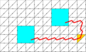
Figure 4: (Color online) A $Z_{2}$-gauge configuration with two identical holes on a torus that contains a $Z_{2}$-monodromy defect in each hole. Such a $Z_{2}$-gauge configuration has $U(-1)=-1$ (each yellow triangle contributes a factor $-1$) (see Fig. 3).

V.1 Bosonic $Z_{n}$ SPT state in 2+1D

We have shown that, in a non-trivial 2+1D $Z_{n}$ SPT state labeled by $m\in{\cal H}^{3}(Z_{n},\mathbb{R}/\mathbb{Z}),\ \ m\neq 0$, $n$ identical $Z_{n}$ monodromy defects will carry a total $Z_{n}$-charge $2m$ mod $n$ (see section III.1.3). We may realize the $n$ identical $Z_{n}$ monodromy defects through $n$ large holes in the 2D space (see Fig. 4). Let us assume that the $Z_{n}$ symmetry is not spontaneously broken at the edge of the holes. Then depending on if a hole contains a $Z_{n}$-monodromy defect or not, the $Z_{n}$-charge of the hole will be $2m/n$ or $0$.

In the large hole limit, adding a monodromy defect to a hole correspond to twisting the boundary condition as we go around the edge of the hole. Such a twist of boundary condition costs zero energy in the large hole limit, (since the branch cut of a monodromy defect costs no energy). If twisting the boundary condition around the edge change the $Z_{n}$-charge on the edge by $2m/n$, then we will change the $Z_{n}$-charge on the edge by $2m$ if we make $n$ identical twists of the boundary condition around the edge. Since twists cost zero energy and $n$ twists are equivalent to no twist, this way, we show that

SPT invariant 31:

the edge of 2+1D $Z_{n}$ SPT state labeled by $m\in{\cal H}^{3}(Z_{n},\mathbb{R}/\mathbb{Z})$ contains nearly degenerate ground states that carry different $Z_{n}$-charges (by $2m$) in the large edge limit.

According to the above result, when $n$=odd, there will be (at least) $n$-fold degenerate edge states, and when $n$=even, there will be (at least) $n/2$-fold degenerate edge states.

So the edge states of the holes must be gapless or degenerate, at least when $n>2$. Also the gapless low energy excitations or the degenerate states must transform non-trivially under the the $Z_{n}$ symmetry transformations. In LABEL:LG1220,L1355, using the non-trivial statistics of the monodromy defects, one can argue more generally that edge states of the holes must be gapless or degenerate even for $n=2$ case.

V.2 Bosonic $Z_{n}$ SPT state in 4+1D

Next, we consider bosonic $Z_{n}$ SPT state in 4+1D, labeled by $m\in{\cal H}^{5}(Z_{n},\mathbb{R}/\mathbb{Z}),\ \ m\neq 0$. We assume the space to have a topology $M_{2}\times M_{2}^{\prime}$. We have shown that, $n$ identical $Z_{n}$ monodromy defects in $M_{2}^{\prime}$ will will induce a 2+1D $Z_{n}$ SPT state on $M_{2}$, labeled by $3m\in{\cal H}^{3}(Z_{n},\mathbb{R}/\mathbb{Z})$ (see section III.1.6). Again, we can realize the $n$ identical $Z_{n}$ monodromy defects through $n$ large holes on $M_{2}^{\prime}$ and assume that the $Z_{n}$ symmetry is not spontaneously broken at the edge of the holes. Then depending on if each hole contains a $Z_{n}$-monodromy defect or not, the 2+1D $Z_{n}$ SPT state on $M_{2}$ will be labeled by $3m$ or $0$ in ${\cal H}^{3}(Z_{n},\mathbb{R}/\mathbb{Z})$. We see that twisting the boundary condition around the edges of the $n$ holes change the 2+1D $Z_{n}$ SPT state on $M_{2}$. Since each twist costs no energy in the large hole limit, the edge states of a hole must be gapless or degenerate, at least when mod$(3m,n)\neq 0$.

V.3 $U(1)$ SPT state in 2+1D and beyond

Figure 5: (Color online) The circle represents $2\pi n$ flux which induce an integer $U(1)$-charge. As we move the flux into the hole, the induced $U(1)$ charge disappears.

We have discussed bosonic and fermionic $U(1)$ SPT states in 2+1D. Those $U(1)$ SPT states are characterized by a non-zero Hall conductance. In LABEL:L8132,W9125, it was shown that a non-zero Hall conductance implies gapless edge excitations. Here we will review the argument.

We consider a 2D space with a hole and $2\pi n$ flux far away from the hole. We assume that there is no $U(1)$ symmetry breaking. The $2\pi n$ flux will induce a non-zero charge $Q=nm$, $m\in\mathbb{Z}$. As we move the $2\pi n$ flux into the hole, the induced $U(1)$-charge will become the charge on the edge. Since $2\pi n$ flux in the hole do not change the boundary condition, the induced $U(1)$-charge is an excitations of the edge.

If the $2\pi n$ flux is generate by a weak field, moving the $2\pi n$ flux into the hole represents a weak perturbation. Since the weak perturbation causes a finite change in the induced charge and also since there are infinite many weak perturbations cause infinite many different change in the induced charges, the excitations on the edge of the hole is gapless.

We can also use a similar argument to show that

SPT invariant 32:

non-trivial bosonic and fermionic $U(1)$ SPT states have gapless boundary excitations in any dimensions.

VI SPT invariants of SPT states with symmetry $G=GG\rtimes SG$

In this section, we will discuss some examples of SPT states where the symmetry group has a form $G=GG\times SG$.

VI.1 Bosonic $U(1)\rtimes Z_{2}$ SPT phases

Let us first consider bosonic $U(1)\rtimes Z_{2}$ SPT phases. We note that $U(1)\rtimes Z_{2}$ is a subgroup of $SO(3)$. So the $U(1)\rtimes Z_{2}$ SPT phases can be realized by spin systems where the spin rotation symmetry is partially broken.

VI.1.1 1+1D

The SPT states with a non-Abelian symmetry $U(1)\rtimes Z_{2}$ in 1+1 dimensions are described by ${\cal H}^{2}[U(1)\rtimes Z_{2},\mathbb{R}/\mathbb{Z}]=\mathbb{Z}_{2}$, whose elements can be labeled by a subset of $\{(m_{0},m_{1},m_{2})\}$, according to the result in appendix D:

$$m_{0} \in{\cal H}^{2}(Z_{2},\mathbb{R}/\mathbb{Z})=\mathbb{Z}_{1},$$

$$m_{1} \in{\cal H}^{1}(Z_{2},{\cal H}^{1}[U(1),\mathbb{R}/\mathbb{Z}]_{Z_{2}})={\cal H}^{1}(Z_{2},\mathbb{Z}_{Z_{2}})=\mathbb{Z}_{2},$$

$$m_{2} \in{\cal H}^{2}(Z_{2},\mathbb{R}/\mathbb{Z})=\mathbb{Z}_{1}.$$ (108)

The second equation in the above is obtained by noting that the nonhomogenous cocycle $\omega_{1}(\theta)\in{\cal H}^{1}[U(1),\mathbb{R}/\mathbb{Z}]\cong\mathbb{Z}$ has a form $\omega_{1}(\theta)=m\frac{\theta}{2\pi}$, $m\in\mathbb{Z}$ [i.e. $\hskip 1.0pt\mathrm{e}^{\hskip 1.0pt\mathrm{i}\hskip 1.0pt2\pi\omega_{1}(\theta)}$ forms a 1D representation of the $U(1)$]. Under the $Z_{2}$ transformation $g$, $\omega_{1}(\theta)$ transforms as $\omega_{1}(\theta)\to\omega_{1}(g\theta g^{-1})=-\omega_{1}(\theta)$ or $m\to-m$, since $g\theta g^{-1}=-\theta$. Therefore, $Z_{2}$ has a non-trivial action on ${\cal H}^{1}[U(1),\mathbb{R}/\mathbb{Z}]=\mathbb{Z}$. We rewrite $\mathbb{Z}$ as $\mathbb{Z}_{Z_{2}}$ and ${\cal H}^{1}[U(1),\mathbb{R}/\mathbb{Z}])$ as ${\cal H}^{1}[U(1),\mathbb{R}/\mathbb{Z}]_{Z_{2}}$ to indicate such a non-trivial action.

Note that ${\cal H}^{1}(Z_{2},\mathbb{Z})=\mathbb{Z}_{1}$ while ${\cal H}^{1}(Z_{2},\mathbb{Z}_{Z_{2}})=\mathbb{Z}_{2}$. This is because the cocycle condition for ${\cal H}^{1}(Z_{2},\mathbb{Z}_{Z_{2}})$ is

$$(\hskip 1.0pt\mathrm{d}\omega_{1})(g_{0},g_{1}) =g_{0}\cdot\omega_{1}(g_{1})-\omega_{1}(g_{0}g_{1})+\omega_{1}(g_{0})=0,$$

$$g_{0},g_{1} \in Z_{2}=\{1,-1\}.$$ (109)

Using $g_{0}\cdot\omega_{1}(g_{1})=\pm\omega_{1}(g_{1})$ when $g_{0}=\pm 1$, we can reduce the above to

$$\omega_{1}(1)=0,\ \ \ -\omega_{1}(-1)-\omega_{1}(1)+\omega_{1}(-1)=0.$$ (110)

So the cocycles are given by

$$\omega_{1}(1)=0,\ \ \ \omega_{1}(-1)=\text{integer}.$$ (111)

The 1-coboundaries are given by

$$(\hskip 1.0pt\mathrm{d}\omega_{0})(g_{0})=g_{0}\cdot\omega_{0}-\omega_{0}$$ (112)

or

$$(\hskip 1.0pt\mathrm{d}\omega_{0})(1)=0,\ \ \ (\hskip 1.0pt\mathrm{d}\omega_{0})(-1)=\text{even integer}.$$ (113)

We see that ${\cal H}^{1}(Z_{2},\mathbb{Z}_{Z_{2}})=\mathbb{Z}_{2}$.

We also note that every elements in ${\cal H}^{2}[U(1)\rtimes Z_{2},\mathbb{R}/\mathbb{Z}]$ can be labeled by at least one $(m_{0},m_{1},m_{2})$, but it is possible that not every $(m_{0},m_{1},m_{2})$ labels an element in ${\cal H}^{2}[U(1)\rtimes Z_{2},\mathbb{R}/\mathbb{Z}]$. In other word, the two sets, $\{(m_{0},m_{1},m_{2})\}$ and ${\cal H}^{2}[U(1)\rtimes Z_{2},\mathbb{R}/\mathbb{Z}]$, are related by a sequence

$$\{(m_{0},m_{1},m_{2})\}\to{\cal H}^{2}[U(1)\rtimes Z_{2},\mathbb{R}/\mathbb{Z}]\to 0.$$ (114)

In this particular case, since $\{m_{0}\}=\{m_{2}\}=\mathbb{Z}_{1}$, we know that $\{m_{1}\}=\mathbb{Z}_{2}$ and ${\cal H}^{2}[U(1)\rtimes Z_{2},\mathbb{R}/\mathbb{Z}]$ has an one-to-one correspondence.

To measure $m_{1}$, we put the system on a finite line $I_{1}$. At an end of the line, we get degenerate states that form a projective representation of $U(1)\rtimes Z_{2}$,Chen et al. (2011a); Schuch et al. (2011); Chen et al. (2011b) if $m_{1}\neq 0$. If we view $U(1)\rtimes Z_{2}$ as a subgroup of $SO(3)$, the projective representations of $U(1)\rtimes Z_{2}$ are simply half-integer spin representations of $SO(3)$.

One way to understand such a result is to gauge the $U(1)\rtimes Z_{2}$ symmetry, the $U(1)\rtimes Z_{2}$ SPT states are described are described by the following gauge topological term (induced by integrating out the matter fields)

$${\cal L}_{\text{top}}=\frac{m_{1}}{2}F$$ (115)

where $F$ is the field strength two form for the $U(1)$-gauge field. Under $Z_{2}$ transformation, $F\to-F$. Since $\int_{M_{2}}\frac{m_{1}}{2}F=m_{1}\pi$ on any closed 1+1D space-time manifold $M_{2}$, ${\cal L}_{\text{top}}$ respects the $Z_{2}$ symmetry, since $m_{1}$ is an integer.

If the space-time $M_{2}$ has a boundary, the above topological term naively reduce to an effective Lagrangian on the boundary

$${\cal L}_{0+1D}=\frac{m_{1}}{2}A$$ (116)

where $A$ is the gauge potential one form. This is nothing but a 1D $U(1)$ Chern-Simons term with a fractional coefficient. But such a 1D $U(1)$ Chern-Simons term breaks the $Z_{2}$ symmetry. So only if the $Z_{2}$ symmetry is broken at the boundary, can the topological term reduce to the 1D Chern-Simons term on the boundary. If the $Z_{2}$ symmetry is not broken, we have the following effective boundary theory

$${\cal L}_{0+1D}=\frac{m_{1}\sigma}{2}A+{\cal L}(\sigma)$$ (117)

where the $\sigma(x)$ field only takes two values $\sigma=\pm 1$. We see that if $m_{1}=0$, the ground state of the 0+1D system is not degenerate $|\text{ground}\rangle=|\sigma=1\rangle+|\sigma=-1\rangle$. If $m_{1}=1$, the ground states of the 0+1D system is degenerate, which are described by $|\sigma=\pm 1\rangle$ states carrying fractional $\pm 1/2$ $U(1)$-charges. Such states form a projective representation of $U(1)\rtimes Z_{2}$.

We can also view the $U(1)\rtimes Z_{2}$ SPT states as $Z_{2}\times Z_{2}$ SPT states. Using the results in SPT invariant 16, we find that

SPT invariant 33:

Consider a 1+1D bosonic $U(1)\rtimes Z_{2}$ SPT state labeled by $m_{1}\in{\cal H}^{2}(U(1)\rtimes Z_{2},\mathbb{R}/\mathbb{Z})$. If we put the SPT state on a circle $S_{1}$, adding $\pi$-flux of $U(1)$ through $S_{1}$ will induce a $Z_{2}$-charge $m_{1}$, and adding $\pi$-flux of $Z_{2}$ through $S_{1}$ will induce a $U(1)$-charge $m_{1}+$even integers in the ground state.

VI.1.2 2+1D

The $U(1)\rtimes Z_{2}$ SPT states in 2+1 dimensions are described by ${\cal H}^{3}[U(1)\rtimes Z_{2},\mathbb{R}/\mathbb{Z}]=\mathbb{Z}_{2}$, whose elements can be labeled by a subset of $\{(m_{0},m_{1},m_{2},m_{3})\}$ (see appendix D), where

$$m_{0} \in{\cal H}^{3}[U(1),\mathbb{R}/\mathbb{Z}]=\mathbb{Z},$$

$$m_{1} \in{\cal H}^{1}(Z_{2},{\cal H}^{2}[U(1),\mathbb{R}/\mathbb{Z}])={\cal H}^{1}(Z_{2},\mathbb{Z}_{1})=\mathbb{Z}_{1},$$

$$m_{2} \in{\cal H}^{2}(Z_{2},{\cal H}^{1}[U(1),\mathbb{R}/\mathbb{Z}]_{Z_{2}})={\cal H}^{2}(Z_{2},\mathbb{Z}_{Z_{2}})=\mathbb{Z}_{1},$$

$$m_{3} \in{\cal H}^{2}(Z_{2},\mathbb{R}/\mathbb{Z})=\mathbb{Z}_{2}.$$ (118)

We see that the 2+1D $U(1)\rtimes Z_{2}$ SPT states can be viewed as 2+1D $U(1)$ SPT states (described by ${\cal H}^{3}[U(1),\mathbb{R}/\mathbb{Z}]=\mathbb{Z}$) or 2+1D $Z_{2}$ SPT states (described by ${\cal H}^{3}[Z_{2},\mathbb{R}/\mathbb{Z}]=\mathbb{Z}_{2}$). Their SPT invariants have been discussed before.

VI.1.3 3+1D

The 3+1D $U(1)\rtimes Z_{2}$ SPT states are described by ${\cal H}^{4}[U(1)\rtimes Z_{2},\mathbb{R}/\mathbb{Z}]=\mathbb{Z}_{2}$, whose elements can be labeled by a subset of $\{(m_{0},m_{1},m_{2},m_{3},m_{4})\}$ (see appendix D), where

$$m_{0} \in{\cal H}^{4}[U(1),\mathbb{R}/\mathbb{Z}]=\mathbb{Z}_{1},$$

$$m_{1} \in{\cal H}^{1}(Z_{2},{\cal H}^{3}[U(1),\mathbb{R}/\mathbb{Z}])={\cal H}^{1}(Z_{2},\mathbb{Z})=\mathbb{Z}_{1},$$

$$m_{2} \in{\cal H}^{2}(Z_{2},{\cal H}^{2}[U(1),\mathbb{R}/\mathbb{Z}])={\cal H}^{2}(Z_{2},\mathbb{Z}_{1})=\mathbb{Z}_{1},$$

$$m_{3} \in{\cal H}^{3}(Z_{2},{\cal H}^{1}[U(1),\mathbb{R}/\mathbb{Z}]_{Z_{2}})={\cal H}^{3}(Z_{2},\mathbb{Z}_{Z_{2}})=\mathbb{Z}_{2},$$

$$m_{4} \in{\cal H}^{4}(Z_{2},\mathbb{R}/\mathbb{Z})=\mathbb{Z}_{1}.$$ (119)

Note that $Z_{2}$ has a trivial action on ${\cal H}^{3}[U(1),\mathbb{R}/\mathbb{Z}]$. To construct the SPT invariants that probe $m_{3}$, we can view the $U(1)\rtimes Z_{2}$ SPT states as $Z_{2}\times Z_{2}$ SPT states and use the result in section IV.5.3. This is because, as we replace $U(1)$ by $Z_{2}$, ${\cal H}^{3}(Z_{2},{\cal H}^{1}[U(1),\mathbb{R}/\mathbb{Z}]_{Z_{2}})$ becomes ${\cal H}^{3}[Z_{2},{\cal H}^{1}(Z_{2},\mathbb{R}/\mathbb{Z})]=\mathbb{Z}_{2}$. In section IV.5.3, we have discussed how to measure ${\cal H}^{3}[Z_{2},{\cal H}^{1}(Z_{2},\mathbb{R}/\mathbb{Z})]$. The same set up also measure ${\cal H}^{3}(Z_{2},{\cal H}^{1}[U(1),\mathbb{R}/\mathbb{Z}]_{Z_{2}})$. This allow us to obtain the following result.

SPT invariant 34:

Consider a 3+1D bosonic $U(1)\rtimes Z_{2}$ SPT state labeled by $m_{3}\in{\cal H}^{4}(U(1)\rtimes Z_{2},\mathbb{R}/\mathbb{Z})$. If we put the SPT state on a space with topology $S_{1}\times M_{2}$, adding $\pi$-flux of $U(1)$ through $S_{1}$ will induce a bosonic $Z_{2}$ SPT state in the 2D space labeled by $m_{3}$ in ${\cal H}^{3}(Z_{2},\mathbb{R}/\mathbb{Z})$. This also implies that a $\pi$-flux vortex line in $U(1)$ will carry the gapless/degenerate edge statesChen and Wen (2012) of the 2+1D bosonic $Z_{2}$ SPT state labeled by $m_{3}$ in ${\cal H}^{3}(Z_{2},\mathbb{R}/\mathbb{Z})$.

VI.2 Bosonic $U_{c}(1)\times[U_{s}(1)\rtimes Z_{2}]$ SPT states

After the preparation of the last section, in this section, we will use the tools (i.e. the SPT invariants) developed so far to study a more complicated example: bosonic $U_{c}(1)\times[U_{s}(1)\rtimes Z_{2}]$ SPT states in various dimensions. We note that $U_{s}(1)\rtimes Z_{2}$ is a subgroup of $SO(3)$. So the results obtained here apply to integer-spin boson gas with boson number conservation. For this reason, we will call $U_{c}(1)$ the charge $U(1)$ and $U_{s}(1)$ the spin $U(1)$.

VI.2.1 1+1D

The different $U_{c}(1)\times[U_{s}(1)\rtimes Z_{2}]$ bosonic SPT states in 1+1D are described by ${\cal H}^{2}[U_{c}(1)\times[U_{s}(1)\rtimes Z_{2}],\mathbb{R}/\mathbb{Z}]$ According to the Künneth formula (see appendix C)

$$\ \ \ \ {\cal H}^{2}[U_{c}(1)\times[U_{s}(1)\rtimes Z_{2}],\mathbb{R}/\mathbb{Z}]$$

$$={\cal H}^{0}(U_{c}(1),{\cal H}^{2}[U_{s}(1)\rtimes Z_{2},\mathbb{R}/\mathbb{Z}])$$

$$={\cal H}^{2}[U_{s}(1)\rtimes Z_{2},\mathbb{R}/\mathbb{Z}]=\mathbb{Z}_{2}=\{m_{0}\},$$ (120)

We see that there are two $U_{c}(1)\times[U_{s}(1)\rtimes Z_{2}]$ bosonic SPT states in 1+1D (including the trivial one), labeled by $m_{0}=0,1$. The SPT states involve only the $U_{s}(1)\rtimes Z_{2}$ symmetry. The non-trivial 1D SPT state carries a projective representation of $U_{s}(1)\rtimes Z_{2}$ at each end if the 1D SPT state form an open chain.Chen et al. (2011a); Schuch et al. (2011); Chen et al. (2011b) This state was discussed in the last section.

VI.2.2 2+1D

Group cohomology description:

The different $U_{c}(1)\times[U_{s}(1)\rtimes Z_{2}]$ bosonic SPT states in 1+1D are described by ${\cal H}^{3}[U_{c}(1)\times[U_{s}(1)\rtimes Z_{2}],\mathbb{R}/\mathbb{Z}]$:

$$\ \ \ \ {\cal H}^{3}[U_{c}(1)\times[U_{s}(1)\rtimes Z_{2}],\mathbb{R}/\mathbb{Z}]$$

$$={\cal H}^{0}(U_{c}(1),{\cal H}^{3}[U_{s}(1)\rtimes Z_{2},\mathbb{R}/\mathbb{Z}])\oplus$$

$$\ \ \ \ {\cal H}^{1}(U_{c}(1),{\cal H}^{2}[U_{s}(1)\rtimes Z_{2},\mathbb{R}/\mathbb{Z}])\oplus$$

$$\ \ \ \ {\cal H}^{2}(U_{c}(1),{\cal H}^{3}[U_{s}(1)\rtimes Z_{2},\mathbb{R}/\mathbb{Z}])\oplus$$

$$\ \ \ \ {\cal H}^{3}(U_{c}(1),{\cal H}^{0}[U_{s}(1)\rtimes Z_{2},\mathbb{R}/\mathbb{Z}]),$$ (121)

where

$$\ \ \ \ {\cal H}^{0}(U_{c}(1),{\cal H}^{3}[U_{s}(1)\rtimes Z_{2},\mathbb{R}/\mathbb{Z}])$$

$$={\cal H}^{3}[U_{s}(1)\rtimes Z_{2},\mathbb{R}/\mathbb{Z}]=\mathbb{Z}\oplus\mathbb{Z}_{2}=\{m_{0},m_{0}^{\prime}\},$$ (122)

$$\ \ \ \ {\cal H}^{1}(U_{c}(1),{\cal H}^{2}[U_{s}(1)\rtimes Z_{2},\mathbb{R}/\mathbb{Z}])$$

$$={\cal H}^{1}[U_{c}(1),\mathbb{Z}_{2}]=0,$$ (123)

$$\ \ \ \ {\cal H}^{2}(U_{c}(1),{\cal H}^{1}[U_{s}(1)\rtimes Z_{2},\mathbb{R}/\mathbb{Z}])$$

$$={\cal H}^{2}[U_{c}(1),\mathbb{Z}_{2}]=\mathbb{Z}_{2}=\{m_{2}\},$$ (124)

$$\ \ \ \ {\cal H}^{3}(U_{c}(1),{\cal H}^{0}[U_{s}(1)\rtimes Z_{2},\mathbb{R}/\mathbb{Z}])$$

$$={\cal H}^{3}[U_{c}(1),\mathbb{R}/\mathbb{Z}]=\mathbb{Z}=\{m_{3}\}.$$ (125)

We see that $U_{c}(1)\times[U_{s}(1)\rtimes Z_{2}]$ bosonic SPT states in 2+1D are labeled by $m_{0},m_{3}\in\mathbb{Z}$ and by $m_{0}^{\prime},m_{2}\in\mathbb{Z}_{2}$.

The $(m_{0},m_{0}^{\prime},m_{2},m_{3})=(m_{0},0,0,0)$ SPT states:

We note that a $(m_{0},0,0,0)$ SPT state is still non-trivial if we break the $Z_{2}$ symmetry and the charge $U(1)$ symmetry since ${\cal H}^{3}[U_{c}(1),\mathbb{R}/\mathbb{Z}]=\mathbb{Z}$ for the spin $U(1)$ symmetry. Thus, if we probe the $(m_{0},0,0,0)$ SPT state by a non-dynamical $U(1)$-gauge field $A_{\mu}$, after we integrate out the matter fields, we will obtain the following quantized gauge topological term in 3+1D:Hung and Wen (2012)

$${\cal L}_{2+1D}=\frac{2m_{0}}{4\pi}A_{\mu}\partial_{\nu}A_{\lambda}\epsilon^{\mu\nu\lambda},$$ (126)

which characterize the $(m_{0},0,0,0)$ SPT state. The Hall conduce for the charge $U(1)$ symmetry is quantized as an even integer $\sigma_{xy}=\frac{2m_{0}}{2\pi}$, which is the SPT invariant that fully characterizes the $(m_{0},0,0,0)$ SPT states.

The $(m_{0},m_{0}^{\prime},m_{2},m_{3})=(0,m_{0}^{\prime},0,0)$ SPT states:

Again, the $(0,m_{0}^{\prime},0,0)$ SPT states only involves the $U_{s}(1)\rtimes Z_{2}$ symmetry. The charge $U(1)$ is not relevant here. So we will drop it in the following discussion. To probe the $(0,m_{0}^{\prime},0,0)$ SPT states, we create two identical monodromy defects of the spin $U(1)$ symmetry, each with a $\pi$ twist. Such monodromy defects do not break the $U_{s}(1)\rtimes Z_{2}$ symmetry. The SPT invariant for the $(0,m_{0}^{\prime},0,0)$ SPT states is the total $Z_{2}$ charge of the two monodromy defects, which is given by $m_{0}^{\prime}$. Such a SPT invariant fully characterizes the $(0,m_{0}^{\prime},0,0)$ SPT states.

In fact, we can view the 2+1D $U_{s}(1)\rtimes Z_{2}$ SPT states as $Z_{2}\times Z_{2}$ SPT states. Then the above SPT invariant is one of those discussed in section IV.5.1.

VI.2.3 3+1D

Group cohomology description:

The different $U_{c}(1)\times[U_{s}(1)\rtimes Z_{2}]$ bosonic SPT states in 3+1D are described by ${\cal H}^{4}[U_{c}(1)\times[U_{s}(1)\rtimes Z_{2}],\mathbb{R}/\mathbb{Z}]$. According to the Künneth formula (see appendix C)

$$\ \ \ \ {\cal H}^{4}[U_{c}(1)\times[U_{s}(1)\rtimes Z_{2}],\mathbb{R}/\mathbb{Z}]$$

$$={\cal H}^{2}(U_{c}(1),{\cal H}^{2}[U_{s}(1)\rtimes Z_{2},\mathbb{R}/\mathbb{Z}])\oplus$$

$$\ \ \ \ {\cal H}^{0}(U_{c}(1),{\cal H}^{4}[U_{s}(1)\rtimes Z_{2},\mathbb{R}/\mathbb{Z}])$$ (127)

where we have only kept the non-zero terms, and

$$\ \ \ \ {\cal H}^{2}(U_{c}(1),{\cal H}^{2}[U_{s}(1)\rtimes Z_{2},\mathbb{R}/\mathbb{Z}])$$

$$={\cal H}^{2}[U_{c}(1),\mathbb{Z}_{2}]=\mathbb{Z}_{2}=\{m_{2}\},$$ (128)

$$\ \ \ \ {\cal H}^{0}(U_{c}(1),{\cal H}^{4}[U_{s}(1)\rtimes Z_{2},\mathbb{R}/\mathbb{Z}])$$

$$={\cal H}^{4}[U_{s}(1)\rtimes Z_{2},\mathbb{R}/\mathbb{Z}]=\mathbb{Z}_{2}=\{m_{0}\}.$$ (129)

We see that there are four $U_{c}(1)\times[U_{s}(1)\rtimes Z_{2}]$ bosonic SPT states in 3+1D (including the trivial one), labeled by $m_{0}=0,1$ and $m_{2}=0,1$. The SPT state $(m_{0},m_{2})=(1,0)$ involves only the $U_{s}(1)\rtimes Z_{2}$ symmetry, which is discussed in section VI.1.3. On the other hand, the $(m_{0},m_{2})=(0,1)$ SPT state involves the full $U_{c}(1)\times[U_{s}(1)\rtimes Z_{2}]$ symmetry and is new.

The $(m_{0},m_{2})=(0,1)$ SPT state:

One way to probe the $(m_{0},m_{2})=(0,1)$ SPT state is to couple the the $U_{c}(1)$ and $U_{s}(1)$ charges to non-dynamical gauge fields $A_{c\mu}$ and $A_{s\mu}$. After we integrate out the matter fields, we will obtain the following quantized gauge topological term in 3+1D:Hung and Wen (2012)

$${\cal L}_{3+1D}=\frac{\pi}{(2\pi)^{2}}\partial_{\mu}A_{c\nu}\partial_{\lambda}A_{s\gamma}\epsilon^{\mu\nu\lambda\gamma}$$ (130)

The structure of the above quantized gauge topological term is consistent with corresponding group cohomology class ${\cal H}^{2}(U_{c}(1),{\cal H}^{2}[U_{s}(1)\rtimes Z_{2},\mathbb{R}/\mathbb{Z}])$.

To understand the physical properties (i.e. the SPT invariants) of the $(m_{0},m_{2})=(0,1)$ SPT state, let us assume that the 3+1D space-time has a topology $M_{2}\times M_{2}^{\prime}$. We also assume that the $A_{c\mu}$ gauge field has $2\pi$ flux on $M_{2}^{\prime}$. In the large $M_{2}$ limit, the Lagrangian (130) reduces to an effective Lagrangian on $M_{2}$ which has a form

$${\cal L}_{M_{2}}=\frac{\pi}{2\pi}\partial_{\mu}A_{s\nu}\epsilon^{\mu\nu}.$$ (131)

We note that the $A_{c\mu}$ gauge configuration preserve the $U_{c}(1)\times(U_{s}(1)\rtimes Z_{2})$ symmetry. The above Lagrangian is the effective Lagrangian of the $U_{c}(1)\times[U_{s}(1)\rtimes Z_{2}]$ symmetric theory on $M_{2}$ probed by the $A_{s\mu}$ gauge field. Such an effective Lagrangian implies that the $U_{s}(1)\rtimes Z_{2}$ symmetric theory on $M_{2}$ describe a non-trivial $U_{s}(1)\rtimes Z_{2}$ SPT state labeled by the non-trivial element $m_{2}=1$ in ${\cal H}^{2}[U_{c}(1)\rtimes Z_{2},\mathbb{R}/\mathbb{Z}]=\mathbb{Z}_{2}$. (The charge $U(1)$ does not play a role here.)

The non-trivial 1+1D $U_{s}(1)\rtimes Z_{2}$ SPT state on $M_{2}$ has the following property: Let $M_{2}=R_{t}\times I$, where $R_{t}$ is the time and $I$ is a spatial line segment. Then the excitations at the end of the line are degenerate, and the degenerate end-states form a projective representation of $U_{s}(1)\rtimes Z_{2}$,Chen et al. (2011a); Schuch et al. (2011); Chen et al. (2011b); Pollmann et al. (2010) provided that the $A_{c\mu}$ gauge field has $2\pi$ flux on $M_{2}^{\prime}$.

The above result has another interpretation. Let the 3+1D space-time has a topology $R_{t}\times I\times M_{2}^{\prime}$. Such a space-time has two boundaries. Each boundary has a topology $R_{t}\times M_{2}^{\prime}$. The above result implies that the excitations on $M_{2}^{\prime}$ form a linear representation of $U_{c}(1)\times[U_{s}(1)\rtimes Z_{2}]$, if the $A_{c\mu}$ gauge field is zero on $M_{2}^{\prime}$. However, the excitations on $M_{2}^{\prime}$ will form a projective representation of $U_{c}(1)\times[U_{s}(1)\rtimes Z_{2}]$, if the $A_{c\mu}$ gauge field has $2\pi$ flux on $M_{2}^{\prime}$. If we shrink the boundary $M_{2}^{\prime}$ to a point, we see that

SPT invariant 35:

the monopole of $A_{c\mu}$ gauge field in the 3+1D $U_{c}(1)\times[U_{s}(1)\rtimes Z_{2}]$ SPT state with $(m_{0},m_{2})=(0,1)$ will carries a projective representation of $U_{s}(1)\rtimes Z_{2}$.

Note that the monopole of charge $A_{c\mu}$ gauge field does not break the $U_{s}(1)\rtimes Z_{2}$ symmetry. If we view $U_{s}(1)\rtimes Z_{2}$ as a subgroup of $SO(3)$, we may say that the monopole of $A_{c\mu}$ gauge field carries a half-integer spin.

Adding $2\pi$ flux of $A_{c\mu}$ gauge field is a weak perturbation if $M_{2}^{\prime}$ is large. Such a perturbation changes the $U_{s}(1)\rtimes Z_{2}$ representation of all the low energy boundary excitations from linear to projective, which implies that the 2+1D boundary $R_{t}\times M_{2}^{\prime}$ has gapless excitations or degenerate ground states. In other words, we can prove the basic conjecture regarding to the boundary of SPT phases, for the case of $U_{c}(1)\times[U_{s}(1)\rtimes Z_{2}]$ SPT state.

VI.3 Bosonic $U(1)\rtimes Z_{2}^{T}$ SPT phases

In this section, we are going to study bosonic $U(1)\rtimes Z_{2}^{T}$ SPT phases. Those SPT phases can be realized by charged bosons with time reversal symmetry.

VI.3.1 1+1D

Let us first consider 1+1D SPT states with symmetry $U(1)\rtimes Z_{2}^{T}$, which are described by ${\cal H}^{2}(U(1)\rtimes Z_{2}^{T},(\mathbb{R}/\mathbb{Z})_{T})=\mathbb{Z}_{2}$. According to the result in appendix D, the elements in ${\cal H}^{2}(U(1)\rtimes Z_{2}^{T},(\mathbb{R}/\mathbb{Z})_{T})$ can be labeled by a subset of $\{(m_{0},m_{1},m_{2})\}$, where

$$m_{0} \in{\cal H}^{0}[Z_{2}^{T},{\cal H}^{2}[U(1),\mathbb{R}/\mathbb{Z}])=\mathbb{Z}_{1},$$ (132)

$$m_{1} \in{\cal H}^{1}[Z_{2}^{T},{\cal H}^{1}[U(1),\mathbb{R}/\mathbb{Z}])={\cal H}^{1}(Z_{2}^{T},\mathbb{Z})=\mathbb{Z}_{1},$$

$$m_{2} \in{\cal H}^{2}[Z_{2}^{T},{\cal H}^{0}[U(1),\mathbb{R}/\mathbb{Z}]_{T})={\cal H}^{2}(Z_{2}^{T},(\mathbb{R}/\mathbb{Z})_{T})=\mathbb{Z}_{2}.$$

where we have use the fact that $Z_{2}^{T}$ has a trivial action on ${\cal H}^{1}[U(1),\mathbb{R}/\mathbb{Z}]$. We see that $m_{2}=0,1$ describes the two 1+1D $U(1)\rtimes Z_{2}^{T}$ SPT states. The $U(1)$ symmetry is irrelevant here. Therefore,

SPT invariant 36:

a 1+1D bosonic $U(1)\rtimes Z_{2}^{T}$ SPT state labeled by $m_{2}=1$ has a degenerate Kramer doublet at an open boundary.

VI.3.2 2+1D

Next, we consider the $U(1)\rtimes Z_{2}^{T}$ SPT states in 2+1 dimensions, which are described by ${\cal H}^{3}(U(1)\rtimes Z_{2}^{T},(\mathbb{R}/\mathbb{Z})_{T})=\mathbb{Z}\oplus\mathbb{Z}_{2}$. The elements in ${\cal H}^{3}(U(1)\rtimes Z_{2}^{T},(\mathbb{R}/\mathbb{Z})_{T})$ can be labeled by a subset of $\{(m_{0},m_{1},m_{2},m_{3})\}$ (see appendix D), where

$$m_{0} \in{\cal H}^{0}[Z_{2}^{T},{\cal H}^{3}[U(1),\mathbb{R}/\mathbb{Z}]_{T})={\cal H}^{0}(Z_{2}^{T},\mathbb{Z}_{T})=\mathbb{Z}_{1},$$

$$m_{1} \in{\cal H}^{1}[Z_{2}^{T},{\cal H}^{2}[U(1),\mathbb{R}/\mathbb{Z}])=\mathbb{Z}_{1},$$ (133)

$$m_{2} \in{\cal H}^{2}[Z_{2}^{T},{\cal H}^{1}[U(1),\mathbb{R}/\mathbb{Z}])$$

$$={\cal H}^{1}(Z_{2}^{T},\mathbb{R}/\mathbb{Z})\otimes_{\mathbb{Z}}{\cal H}^{1}[U(1),\mathbb{R}/\mathbb{Z}])=\mathbb{Z}_{2},$$

$$m_{3} \in{\cal H}^{3}[Z_{2}^{T},{\cal H}^{0}[U(1),\mathbb{R}/\mathbb{Z}]_{T})={\cal H}^{3}(Z_{2}^{T},(\mathbb{R}/\mathbb{Z})_{T})=\mathbb{Z}_{1},$$

where we have use the fact that $Z_{2}^{T}$ has a trivial action on ${\cal H}^{1}[U(1),\mathbb{R}/\mathbb{Z}]$ and a non-trivial action on ${\cal H}^{3}[U(1),\mathbb{R}/\mathbb{Z}]$. We see that the $U(1)\rtimes Z_{2}^{T}$ SPT states are described by $m_{2}=0,1$.

To measure $m_{2}$, we note that if we break the $U(1)$ symmetry down to $Z_{2}$, we the non-trivial SPT state with $m_{2}=1$ is still non-trivial, since ${\cal H}^{2}[Z_{2}^{T},{\cal H}^{1}[U(1),\mathbb{R}/\mathbb{Z}])={\cal H}^{2}[Z_{2}^{T},{\cal H}^{1}(Z_{2},\mathbb{R}/\mathbb{Z})_{T}]=Z_{2}$. If we also break the $Z_{2}^{T}$ symmetry at the same time, the $U(1)\rtimes Z_{2}^{T}$ SPT state described by $m_{2}=1$ will become a trivial $Z_{2}$ SPT state. So the $U(1)\rtimes Z_{2}^{T}$ SPT state described by $m_{2}=1$ is also a non-trivial $Z_{2}\times Z_{2}^{T}$ SPT state. The above consideration suggest that such a $Z_{2}\times Z_{2}^{T}$ SPT state is described by a non-trivial $m_{1}$ in eqn. (IV.8.2). So we can use the SPT invariant that detect $m_{1}$ of the $Z_{2}\times Z_{2}^{T}$ SPT states to detect $m_{2}$ of the $U(1)\rtimes Z_{2}^{T}$ SPT states. Thus

SPT invariant 37:

Consider a 2+1D bosonic $U(1)\rtimes Z_{2}^{T}$ SPT state labeled by $m_{2}=1$ in ${\cal H}^{3}(U(1)\rtimes Z_{2}^{T},(\mathbb{R}/\mathbb{Z})_{T})$ . If we put the state on a cylinder $I\times S_{1}$, then the states on one boundary will form Kramer doublets, if we twist the boundary condition around $S_{1}$ by the $\pi$ rotation in $U(1)$. This also implies that a $U(1)$ monodromy defect generated by $\pi$ rotation carries a degenerate Kramer doublet.

Table 1: Symmetry-protected topological invariants for various bosonic SPT states. Here the flux, the monodromy defects and the monopoles are always the minimal ones. $\{n_{1},n_{2}\}$ is the smallest common multiple of $n_{1},n_{2}$. $\langle n_{1},n_{2}\rangle$ is the largest common divisor of $n_{1},n_{2}$. Also ${\cal H}^{d}(G)\equiv{\cal H}^{d}(G,\mathbb{R}/\mathbb{Z})$. The previously known results are indicated by the references.

symmetry	dim.	labels	symmetry-protected topological invariants
$Z_{n}$	2+1D	$m\in{\cal H}^{3}(Z_{n})=\mathbb{Z}_{n}$	$\bullet$ $n$ identical monodromy defects have a total $Z_{n}$ charge $2m$. $\bullet$ A monodromy defect has a statistics $\theta=2\pi(\frac{m}{n^{2}}+\frac{\text{integer}}{n})$.Levin and Gu (2012); Mesaros and Ran (2013); Hung and Wen (2013)
$U(1)$	2+1D	$m\in{\cal H}^{3}[U(1)]=\mathbb{Z}$	$\bullet$ Even-integer quantized Hall conductance $\sigma_{xy}=2m/2\pi$.Lu and Vishwanath (2012); Liu and Wen (2013); Chen and Wen (2012); Senthil and Levin (2013)
	1+1D	$m_{1}\in{\cal H}^{1}(Z_{n_{1}})\boxtimes_{\mathbb{Z}}{\cal H}^{1}(Z_{n_{2}})=\mathbb{Z}_{\langle n_{1},n_{2}\rangle}$	$\bullet$ The degenerate states at an end of chain form the $m_{1}^{\text{th}}$ projective representation of $Z_{n_{1}}\times Z_{n_{2}}$. $\bullet$ The $Z_{n_{1}}$-flux through the 1D circular space induces a $Z_{n_{2}}$-charge $m+\langle n_{1},n_{2}\rangle\times$ integer.
$Z_{n_{1}}\times Z_{n_{2}}$	2+1D	$m_{0}\in{\cal H}^{3}[Z_{n_{2}}]=\mathbb{Z}_{n_{2}}$ $m_{2}\in{\cal H}^{1}(Z_{n_{1}})\otimes_{\mathbb{Z}}{\cal H}^{1}(Z_{n_{2}})=\mathbb{Z}_{\langle n_{1},n_{2}\rangle}$ $m_{3}\in{\cal H}^{3}(Z_{n_{1}})=\mathbb{Z}_{n_{1}}$	$\bullet$ The statistics of $Z_{n_{1}}$ monodromy defects: $\theta_{11}$ mod $\frac{2\pi}{n_{1}}=\frac{2\pi m_{3}}{n_{1}^{2}}$. The statistics of $Z_{n_{2}}$ monodromy defects: $\theta_{22}$ mod $\frac{2\pi}{n_{2}}=\frac{2\pi m_{0}}{n_{2}^{2}}$. The mutual statistics between $Z_{n_{1}}$ and $Z_{n_{2}}$ monodromy defects: $\theta_{12}$ mod $\frac{2\pi}{\{n_{1},n_{2}\}}=\frac{2\pi m_{2}}{n_{1}n_{2}}$.Levin and Gu (2012); Mesaros and Ran (2013); Hung and Wen (2013) $\bullet$ $n_{1}$ identical $Z_{n_{1}}$ monodromy defects carry $2m_{3}$ $Z_{n_{1}}$ charges and $m_{2}+\langle n_{1},n_{2}\rangle\times$ integer $Z_{n_{2}}$ charges. $n_{2}$ identical $Z_{n_{2}}$ monodromy defects carry $2m_{0}$ $Z_{n_{2}}$ charges and $m_{2}+\langle n_{1},n_{2}\rangle\times$ integer $Z_{n_{1}}$ charges.
	3+1D	$m_{1}\in{\cal H}^{1}(Z_{n_{1}})\boxtimes_{\mathbb{Z}},{\cal H}^{3}(Z_{n_{2}})=\mathbb{Z}_{\langle n_{1},n_{2}\rangle}$ $m_{3}\in{\cal H}^{3}(Z_{n_{1}})\boxtimes_{\mathbb{Z}}{\cal H}^{1}(Z_{n_{2}})=\mathbb{Z}_{\langle n_{1},n_{2}\rangle}$	$\bullet$ A $Z_{n_{1}}$ monodromy line-defect will carry gapless/degenerate edge states of $m_{1}^{\text{th}}$ 2+1D bosonic $Z_{n_{2}}$ SPT states. A $Z_{n_{2}}$ monodromy line-defect will carry gapless/degenerate edge states of $m_{3}^{\text{th}}$ 2+1D bosonic $Z_{n_{1}}$ SPT states.
	1+1D	$m_{1}\in{\cal H}^{1}(Z_{2},{\cal H}^{1}[U(1)]_{Z_{2}})=\mathbb{Z}_{2}$	$\bullet$ A degenerate $U(1)$-charge $\pm 1/2$ doublet at a boundary, if $m_{1}=1$.
$U(1)\rtimes Z_{2}$	2+1D	$m_{0}\in{\cal H}^{3}[U(1)]=\mathbb{Z}$ $m_{3}\in{\cal H}^{3}(Z_{2})=\mathbb{Z}_{2}$	$\bullet$ Same as the $U(1)$ or the $Z_{2}$ SPT states in 2+1D.
	3+1D	$m_{3}\in{\cal H}^{3}(Z_{2},{\cal H}^{1}[U(1)]_{Z_{2}})=\mathbb{Z}_{2}$	$\bullet$ A $\pi$-flux line of the $U(1)$ will carry gapless/degenerate edge states of the 2+1D bosonic $Z_{2}$ SPT state, if $m_{3}=1$.
	1+1D	$m_{2}\in{\cal H}^{2}(Z_{2}^{T},{\cal H}^{0}[U(1)]_{T})=\mathbb{Z}_{2}$	$\bullet$ A neutral Kramer doublet at a boundary, if $m_{2}=1$.
	2+1D	$m_{2}\in{\cal H}^{1}(Z_{2}^{T})\otimes_{\mathbb{Z}}{\cal H}^{1}[U(1)]=\mathbb{Z}_{2}$	$\bullet$ A monodromy defect generated by $U(1)$ $\pi$-rotation carries a degenerate Kramer double, if $m_{2}=1$.
$U(1)\rtimes Z_{2}^{T}$	3+1D	$m_{1}\in{\cal H}^{1}(Z_{2}^{T},{\cal H}^{3}[U(1)]_{T})=\mathbb{Z}_{2}$ $m_{4}\in{\cal H}^{4}[Z_{2}^{T},(\mathbb{R}/\mathbb{Z})_{T}]=\mathbb{Z}_{2}$	$\bullet$ A dyon of (electric,magnetic) charge ($q$,$m$) has a statistics $(-)^{m(q-m_{1}m)}$.Metlitski et al. (2013) $\bullet$ A gapped time-reversal symmetry breaking boundary has a Hall conductance $\sigma_{xy}=\frac{m_{1}}{2\pi}+\frac{\text{even}}{2\pi}$.Vishwanath and Senthil (2013)
	1+1D	$m_{0}\in{\cal H}^{2}[Z_{2}^{T},(\mathbb{R}/\mathbb{Z})_{T}]=\mathbb{Z}_{2}$ $m_{2}\in{\cal H}^{1}[U(1)]\otimes_{\mathbb{Z}}{\cal H}^{0}[Z_{2}^{T},(\mathbb{R}/\mathbb{Z})_{T}]=\mathbb{Z}_{2}$	$\bullet$ A neutral Kramer doublet at a boundary, if $(m_{0},m_{2})=(1,0)$. $\bullet$ A degenerate boundary charge-$\pm\frac{1}{2}$ doublet, if $(m_{0},m_{2})=(0,1)$.
$U(1)\times Z_{2}^{T}$	3+1D	$m_{0}\in{\cal H}^{4}[Z_{2}^{T},(\mathbb{R}/\mathbb{Z})_{T}]=\mathbb{Z}_{2}$ $m_{2}\in{\cal H}^{1}[U(1)]\otimes_{\mathbb{Z}}{\cal H}^{2}[Z_{2}^{T},(\mathbb{R}/\mathbb{Z})_{T}]=\mathbb{Z}_{2}$ $m_{4}\in{\cal H}^{3}[U(1)]\otimes_{\mathbb{Z}}{\cal H}^{0}[Z_{2}^{T},(\mathbb{R}/\mathbb{Z})_{T}]=\mathbb{Z}_{2}$	$\bullet$ A $U(1)$ monopole will carries a neutral degenerate Kramer doublet, if $(m_{1},m_{2},m_{4})=(0,1,0)$. $\bullet$ A dyon of (electric,magnetic) charge ($q$,$m$) has a statistics $(-)^{m(q-m_{4}m)}$, if $(m_{1},m_{2},m_{4})=(0,0,m_{4})$. $\bullet$ A gapped time-reversal symmetry breaking boundary has a Hall conductance $\sigma_{xy}=\frac{m_{4}}{2\pi}+\frac{\text{even}}{2\pi}$.
	1+1D	$m_{0}\in{\cal H}^{2}[Z_{2}^{T},(\mathbb{R}/\mathbb{Z})_{T}]=\mathbb{Z}_{2}$ $m_{2}\in{\cal H}^{1}[U(1)]\otimes_{\mathbb{Z}}{\cal H}^{0}[Z_{2}^{T},(\mathbb{R}/\mathbb{Z})_{T}]=\mathbb{Z}_{2}$	$\bullet$ A neutral Kramer doublet at a boundary, if $(m_{0},m_{2})=(1,0)$. $\bullet$ A degenerate boundary charge-$\pm\frac{1}{2}$ doublet, if $(m_{0},m_{2})=(0,1)$.
	2+1D	$m_{1}\in{\cal H}^{1}(Z_{2})\boxtimes_{\mathbb{Z}}{\cal H}^{2}[Z_{2}^{T},(\mathbb{R}/\mathbb{Z})_{T}]=\mathbb{Z}_{2}$ $m_{3}\in{\cal H}^{3}[Z_{2}]\boxtimes_{\mathbb{Z}}{\cal H}^{0}[Z_{2}^{T},(\mathbb{R}/\mathbb{Z})_{T}]=\mathbb{Z}_{2}$	$\bullet$ A $Z_{2}$ monodromy defect will carries a degenerate Kramer doublet, if $(m_{1},m_{3})=(1,0)$. $\bullet$ $m_{3}$ can be measured as in the 2+1D $Z_{2}$ SPT states.
$Z_{2}\times Z_{2}^{T}$	3+1D	$m_{0}\in{\cal H}^{4}[Z_{2}^{T},(\mathbb{R}/\mathbb{Z})_{T}]=\mathbb{Z}_{2}$ $m_{2}\in{\cal H}^{1}(Z_{2})\otimes_{\mathbb{Z}}{\cal H}^{2}[Z_{2}^{T},(\mathbb{R}/\mathbb{Z})_{T}]=\mathbb{Z}_{2}$ $m_{4}\in{\cal H}^{3}(Z_{2})\otimes_{\mathbb{Z}}{\cal H}^{0}[Z_{2}^{T},(\mathbb{R}/\mathbb{Z})_{T}]=\mathbb{Z}_{2}$	$\bullet$ When $(m_{0},m_{2},m_{4})=(0,0,1)$, the symmetry breaking domain wall in a gapped time-reversal symmetry breaking boundary will carry the edge excitations of the 2+1D $Z_{2}$ STP state. Also the $Z_{2}$ monodromy line-defect will induce two-fold degenerate states with different Z2 charges at its intersection with a gapped time-reversal symmetry breaking boundary, unless the line-defect is gapless. $\bullet$ When $(m_{0},m_{2},m_{4})=(0,1,0)$, two identical ends of the line-defects on a compact surface will induce a degenerate Kramer doublet.

VI.3.3 3+1D

Last, we consider the $U(1)\rtimes Z_{2}^{T}$ SPT states in 3+1 dimensions. Several SPT invariants for such states were discussed in LABEL:VS1258,MKF1335. The $U(1)\rtimes Z_{2}^{T}$ SPT states are described by ${\cal H}^{4}(U(1)\rtimes Z_{2}^{T},(\mathbb{R}/\mathbb{Z})_{T})=\mathbb{Z}_{2}\oplus Z_{2}$. The elements in ${\cal H}^{4}(U(1)\rtimes Z_{2}^{T},(\mathbb{R}/\mathbb{Z})_{T})$ can be labeled by a subset of $\{(m_{0},m_{1},m_{2},m_{3},m_{4})\}$ (see appendix D), where

$$m_{0} \in{\cal H}^{0}[Z_{2}^{T},{\cal H}^{4}[U(1),\mathbb{R}/\mathbb{Z}])=\mathbb{Z}_{1},$$

$$m_{1} \in{\cal H}^{1}[Z_{2}^{T},{\cal H}^{3}[U(1),\mathbb{R}/\mathbb{Z}]_{T})={\cal H}^{1}(Z_{2}^{T},\mathbb{Z}_{T})=\mathbb{Z}_{2},$$

$$m_{2} \in{\cal H}^{2}[Z_{2}^{T},{\cal H}^{2}[U(1),\mathbb{R}/\mathbb{Z}])=\mathbb{Z}_{1},$$ (134)

$$m_{3} \in{\cal H}^{3}[Z_{2}^{T},{\cal H}^{1}[U(1),\mathbb{R}/\mathbb{Z}])={\cal H}^{3}(Z_{2}^{T},\mathbb{Z})=\mathbb{Z}_{1},$$

$$m_{4} \in{\cal H}^{4}[Z_{2}^{T},{\cal H}^{0}[U(1),\mathbb{R}/\mathbb{Z}]_{T})={\cal H}^{4}(Z_{2}^{T},(\mathbb{R}/\mathbb{Z})_{T})=\mathbb{Z}_{2},$$

We see that the 3+1D $U(1)\rtimes Z_{2}^{T}$ SPT states are labeled by $m_{1}=0,1$ and $m_{4}=0,1$. $m_{4}$ labels different 3+1D $Z_{2}^{T}$ SPT states where the $U(1)$ symmetry is irrelevant.

To probe $m_{1}$, we may gauge the $U(1)$ symmetry. We believe that the $U(1)\rtimes Z_{2}^{T}$ SPT states labeled by $(m_{1},m_{4})=(m_{1},0)$ are described by the following $U(1)$-gauge topological term

$${\cal L}_{\text{top}}=\frac{m_{1}\pi}{(2\pi)^{2}}F^{2}$$ (135)

Under the $Z_{2}^{T}$ time-reversal transformation, $F^{2}\to-F^{2}$ and $\hskip 1.0pt\mathrm{e}^{\hskip 1.0pt\mathrm{i}\hskip 1.0pt\int_{M_{4}}\frac{m_{1}\pi}{(2\pi)^{2}}F^{2}}\to\hskip 1.0pt\mathrm{e}^{-\hskip 1.0pt\mathrm{i}\hskip 1.0pt\int_{M_{4}}\frac{m_{1}\pi}{2(2\pi)^{2}}F^{2}}$. Since $\int_{M_{4}}\frac{m_{1}\pi}{(2\pi)^{2}}F^{2}=\pi m_{1}\times$ integers, on any closed 3+1D orientable space-time manifold $M_{4}$, the $Z_{2}^{T}$ symmetry is preserved since $m_{1}$ is an integer. $m_{1}$=odd describes the non-trivial 3+1D $U(1)\rtimes Z_{2}^{T}$ SPT state, while $m_{1}$=even describes the trivial SPT state. Now we see that $m_{1}$ can be measured by the statistical effect discussed in LABEL:W7983,GMW8921,MKF1335:

SPT invariant 38:

in a 3+1D bosonic $U(1)\rtimes Z_{2}^{T}$ SPT state labeled by $(m_{1},m_{4})=(m_{1},0)$, a dyon of the $U(1)$ gauge field with ($U(1)$-charge, magnetic charge) = $(q,m)$ has a statistics $(-)^{m(q-m_{1})}$ (where $+\to$ boson and $-\to$ fermion).

If the space-time $M_{4}$ has a boundary, the topological term (135) reduces to an effective Lagrangian on the boundary

$${\cal L}_{2+1D}=\frac{m_{1}}{4\pi}AF,$$ (136)

if the $Z_{2}^{T}$ time-reversal symmetry is broken on the boundary. The above is nothing but a 2+1D $U(1)$ Chern-Simons term with a quantized Hall conductance $\sigma_{xy}=m_{1}/2\pi$.Vishwanath and Senthil (2013) Thus

SPT invariant 39:

in a 3+1D bosonic $U(1)\rtimes Z_{2}^{T}$ SPT state labeled by $(m_{1},m_{4})$, the gapped time-reversal symmetry breaking boundary has a Hall conductance $\sigma_{xy}=\frac{m_{1}}{2\pi}+\frac{\text{even}}{2\pi}$.

If the $Z_{2}^{T}$ symmetry is not broken, we actually have the following effective boundary theory

$${\cal L}_{2+1D}=\frac{m_{1}\sigma}{4\pi}AF+{\cal L}(\sigma)$$ (137)

where the $\sigma(x)$ field only takes two values $\sigma=\pm 1$. The gapless edge states on the domain wall between $\sigma=1$ and $\sigma=-1$ regions may give rise to the gapless boundary excitations on the 2+1D surface.

VII Summary

Table 2: Symmetry-protected topological invariants for some fermionic SPT states.

symmetry	dim.	labels	symmetry-protected topological invariants
$U^{f}(1)$	2+1D	$m\in\mathbb{Z}$	$\bullet$ 8-times-integer quantized Hall conductance $\sigma_{xy}=8m/2\pi$.
$U(1)\times Z_{2}^{f}$	2+1D	$m\in\mathbb{Z}$	$\bullet$ Integer quantized Hall conductance $\sigma_{xy}=m/2\pi$.
$Z_{2}\times Z_{2}^{f}$	2+1D	$m\in\mathbb{Z}_{8}$	$\bullet$ Abelian/non-Abelian statistics and mutual statistics of the $Z_{2}$ and $Z_{2}^{f}$ monodromy defects. $\bullet$ The mutual induced $Z_{2}$ (or $Z_{2}^{f}$) charge by two identical $Z_{2}^{f}$ (or $Z_{2}$) monodromy defects.

Table 3: The fermionic SPT phases with the full symmetry $G_{f}$. Here $0$ means that there is only trivial SPT phase. $\mathbb{Z}_{n}$ means that the non-trivial SPT phases plus the trivial phase are labeled by the elements in $\mathbb{Z}_{n}$.

$G_{f}$	$0+1D$	$1+1D$	$2+1D$	$3+1D$
$Z_{2}^{f}$	$\mathbb{Z}_{2}$	$0$	$0$	$0$
$U^{f}(1)$	$\mathbb{Z}$	$0$	$\mathbb{Z}$	$0$
$U(1)\times U^{f}(1)$	$\mathbb{Z}\oplus\mathbb{Z}$	$0$	$\mathbb{Z}\oplus\mathbb{Z}\oplus\mathbb{Z}$	$0$
$U(1)\times Z^{f}_{2}$	$\mathbb{Z}\oplus\mathbb{Z}_{2}$	$0$	$\mathbb{Z}$	0
$Z_{2}\times Z^{f}_{2}$	$\mathbb{Z}_{2}\oplus\mathbb{Z}_{2}$	$\mathbb{Z}_{2}$	$\mathbb{Z}_{8}$	?

It has been shown that the SPT states and some of the SET states can be described by the cocycles in the group cohomology class ${\cal H}^{d}(G,\mathbb{R}/\mathbb{Z})$.Chen et al. (2013a); Gu and Wen (2012) In this paper, we construct many SPT invariants which allow us to physically measure the cocycles in ${\cal H}^{d}(G,\mathbb{R}/\mathbb{Z})$ fully. The constructed SPT invariants allow us to physically or numerically detect and characterized the SPT states and some of the SET states.

The SPT invariants are constructed by putting the SPT states on a space-time with a topology $M_{k}\times M_{d-1-k}$ and gauging a subgroup $GG$ of the symmetry group $G$. We then put a non-trivial $GG$ gauge configuration on the closed manifold $M_{k}$. When $k=1$, the gauge configuration can be a gauge flux through the ring. When $k=2$, the gauge configuration can be a gauge flux through $M_{2}$ if $GG$ is continuous or a few identical gauge flux through $M_{2}$ (if $GG$ is discrete), etc .

When $M_{d-1-k}$ is large, the SPT states on $M_{k}\times M_{d-1-k}$ can be viewed as a SPT state on $M_{d-1-k}$ with a symmetry $SG$, where $SG$ is a subgroup of $G$ that commute with $GG$. The $SG$ SPT state on $M_{d-1-k}$ is described by ${\cal H}^{d-k}(SG,\mathbb{R}/\mathbb{Z})$. This way, we can measure the the cocycles in ${\cal H}^{d}(G,\mathbb{R}/\mathbb{Z})$ by measuring the the cocycles in ${\cal H}^{d-k}(SG,\mathbb{R}/\mathbb{Z})$. When $d-k=1$, the cocycles in ${\cal H}^{1}(SG,\mathbb{R}/\mathbb{Z})$ can be measured by measuring the $SG$ quantum number of the ground state. When $d-k=2$, we can choose the space-time $M_{d-1-k}$ to have a space described by a finite line. Then the cocycles in ${\cal H}^{2}(SG,\mathbb{R}/\mathbb{Z})$ can be measured by measuring the projective representation of $SG$ at one end of the line.

In Table 1, we list the SPT invariants for some simple bosonic SPT phases. In Table 2, we list the SPT invariants for a few fermionic SPT phases. More SPT invariants are described by the SPT invariant statements in the paper. Those SPT invariants also allow us to understand some of the SPT states for interacting fermions. We list those results in Table 3.Ryu and Zhang (2012); Gu and Levin (2013)

I like to thank Xie Chen, Zheng-Cheng Gu, Max Metlitski, and Juven Wang for many helpful discussions. This research is supported by NSF Grant No. DMR-1005541, NSFC 11074140, and NSFC 11274192. Research at Perimeter Institute is supported by the Government of Canada through Industry Canada and by the Province of Ontario through the Ministry of Research.

Appendix A Group cohomology theory

A.1 Homogeneous group cocycle

In this section, we will briefly introduce group cohomology. The group cohomology class ${\cal H}^{d}(G,\mathbb{M})$ is an Abelian group constructed from a group $G$ and an Abelian group $\mathbb{M}$. We will use “+” to represent the multiplication of the Abelian groups. Each elements of $G$ also induce a mapping $\mathbb{M}\to\mathbb{M}$, which is denoted as

$$g\cdot m=m^{\prime},\ \ \ g\in G,\ m,m^{\prime}\in\mathbb{M}.$$ (138)

The map $g\cdot$ is a group homomorphism:

$$g\cdot(m_{1}+m_{2})=g\cdot m_{1}+g\cdot m_{2}.$$ (139)

The Abelian group $\mathbb{M}$ with such a $G$-group homomorphism, is call a $G$-module.

A homogeneous $d$-cochain is a function $\nu_{d}:G^{d+1}\to\mathbb{M}$, that satisfies

$$\nu_{d}(g_{0},\cdots,g_{d})=g\cdot\nu_{d}(gg_{0},\cdots,gg_{d}),\ \ \ \ g,g_{i}\in G.$$ (140)

We denote the set of $d$-cochains as ${\cal C}^{d}(G,\mathbb{M})$. Clearly ${\cal C}^{d}(G,\mathbb{M})$ is an Abelian group. homogeneous group cocycle

Let us define a mapping $\hskip 1.0pt\mathrm{d}$ (group homomorphism) from ${\cal C}^{d}(G,\mathbb{M})$ to ${\cal C}^{d+1}(G,\mathbb{M})$:

$$(\hskip 1.0pt\mathrm{d}\nu_{d})(g_{0},\cdots,g_{d+1})=\sum_{i=0}^{d+1}(-)^{i}\nu_{d}(g_{0},\cdots,\hat{g}_{i},\cdots,g_{d+1})$$ (141)

where $g_{0},\cdots,\hat{g}_{i},\cdots,g_{d+1}$ is the sequence $g_{0},\cdots,g_{i},\cdots,g_{d+1}$ with $g_{i}$ removed. One can check that $\hskip 1.0pt\mathrm{d}^{2}=0$. The homogeneous $d$-cocycles are then the homogeneous $d$-cochains that also satisfy the cocycle condition

$$\hskip 1.0pt\mathrm{d}\nu_{d}=0.$$ (142)

We denote the set of $d$-cocycles as ${\cal Z}^{d}(G,\mathbb{M})$. Clearly ${\cal Z}^{d}(G,\mathbb{M})$ is an Abelian subgroup of ${\cal C}^{d}(G,\mathbb{M})$.

Let us denote ${\cal B}^{d}(G,\mathbb{M})$ as the image of the map $\hskip 1.0pt\mathrm{d}:{\cal C}^{d-1}(G,\mathbb{M})\to{\cal C}^{d}(G,\mathbb{M})$ and ${\cal B}^{0}(G,\mathbb{M})=\{0\}$. The elements in ${\cal B}^{d}(G,\mathbb{M})$ are called $d$-coboundary. Since $\hskip 1.0pt\mathrm{d}^{2}=0$, ${\cal B}^{d}(G,\mathbb{M})$ is a subgroup of ${\cal Z}^{d}(G,\mathbb{M})$:

$${\cal B}^{d}(G,\mathbb{M})\subset{\cal Z}^{d}(G,\mathbb{M}).$$ (143)

The group cohomology class ${\cal H}^{d}(G,\mathbb{M})$ is then defined as

$${\cal H}^{d}(G,\mathbb{M})={\cal Z}^{d}(G,\mathbb{M})/{\cal B}^{d}(G,\mathbb{M}).$$ (144)

We note that the $\hskip 1.0pt\mathrm{d}$ operator and the cochains ${\cal C}^{d}(G,\mathbb{M})$ (for all values of $d$) form a so called cochain complex,

$$\cdots\stackrel{{\scriptstyle\hskip 1.0pt\mathrm{d}}}{{\to}}{\cal C}^{d}(G,\mathbb{M})\stackrel{{\scriptstyle\hskip 1.0pt\mathrm{d}}}{{\to}}{\cal C}^{d+1}(G,\mathbb{M})\stackrel{{\scriptstyle\hskip 1.0pt\mathrm{d}}}{{\to}}\cdots$$ (145)

which is denoted as $C(G,\mathbb{M})$. So we may also write the group cohomology ${\cal H}^{d}(G,\mathbb{M})$ as the standard cohomology of the cochain complex $H^{d}[C(G,\mathbb{M})]$.

A.2 Nonhomogeneous group cocycle

The above definition of group cohomology class can be rewritten in terms of nonhomogeneous group cochains/cocycles. An nonhomogeneous group $d$-cochain is a function $\omega_{d}:G^{d}\to M$. All $\omega_{d}(g_{1},\cdots,g_{d})$ form ${\cal C}^{d}(G,\mathbb{M})$. The nonhomogeneous group cochains and the homogeneous group cochains are related as

$$\nu_{d}(g_{0},g_{1},\cdots,g_{d})=\omega_{d}(g_{01},\cdots,g_{d-1,d}),$$ (146)

with

$$g_{0}=1,\ \ g_{1}=g_{0}g_{01},\ \ g_{2}=g_{1}g_{12},\ \ \cdots\ \ g_{d}=g_{d-1}g_{d-1,d}.$$ (147)

Now the $\hskip 1.0pt\mathrm{d}$ map has a form on $\omega_{d}$:

$$(\hskip 1.0pt\mathrm{d}\omega_{d})(g_{01},\cdots,g_{d,d+1})=g_{01}\cdot\omega_{d}(g_{12},\cdots,g_{d,d+1})$$

$$\ \ \ +\sum_{i=1}^{d}(-)^{i}\omega_{d}(g_{01},\cdots,g_{i-1,i}g_{i,i+1},\cdots,g_{d,d+1})$$

$$\ \ \ +(-)^{d+1}\omega_{d}(g_{01},\cdots,\tilde{g}_{d-1,d})$$ (148)

This allows us to define the nonhomogeneous group $d$-cocycles which satisfy $\hskip 1.0pt\mathrm{d}\omega_{d}=0$ and the nonhomogeneous group $d$-coboundaries which have a form $\omega_{d}=\hskip 1.0pt\mathrm{d}\mu_{d-1}$. In the following, we are going to use nonhomogeneous group cocycles to study group cohomology. Geometrically, we may view $g_{i}$ as living on the vertex $i$, while $g_{ij}$ as living on the edge connecting the two vertices $i$ to $j$.

A.3 “Normalized” cocycles

We know that each elements in ${\cal H}^{d}(G,\mathbb{R}/\mathbb{Z})$ can be represented by many cocycles. In the following, we are going describe a way to simplify the cocycles, so that the simplified cocycles can still represent all the elements in ${\cal H}^{d}(G,\mathbb{R}/\mathbb{Z})$.

The simplification is obtained by considering “normalized” cochains,Hochschild and Serre (1953) which satisfy

$$\omega_{d}(g_{1},\cdots,g_{d})=0,\text{ if one of }g_{i}=1.$$ (149)

One can check that the $\hskip 1.0pt\mathrm{d}$-operator maps a “normalized” cochain to a “normalized” cochain. The group cohomology classes obtained from the ordinary cochains is isomorphic to the group cohomology classes obtained from the “normalized” cochains. Let us use $\bar{\cal C}^{d}(G,\mathbb{M})$, $\bar{\cal Z}^{d}(G,\mathbb{M})$, and $\bar{\cal B}^{d}(G,\mathbb{M})$ to denote the “normalized” cochains, cocycles, and coboundaries. We have ${\cal H}^{d}(G,\mathbb{M})=\bar{\cal Z}^{d}(G,\mathbb{M})/\bar{\cal B}^{d}(G,\mathbb{M})$.

A.4 A “differential form” notation for group cocycles

We know that a cocycle $\omega_{d}$ in ${\cal H}^{d}(G,\mathbb{R}/\mathbb{Z})$ is a linear map that map a $d$-dimensional complex $M$, with $g_{i}$ on the vertices or $g_{ij}$ on the edges, to a mod-1 number in $\mathbb{R}/\mathbb{Z}$. Let us use a “differential form” notation to denote such a map:

$$\int_{M}\omega_{d}(g_{ij})\in\mathbb{R}/\mathbb{Z}.$$ (150)

In the above, we have regarded $\omega_{d}(g_{ij})$ as a function of $g_{ij}$ on the edges. We may also view $\omega_{d}$ as a function of $g_{i}$ on the vertices by replacing $g_{ij}$ by $g_{j}g_{i}^{-1}$: $\omega_{d}(g_{j}g_{i}^{-1})$. A differential form $F$ is a linear map from a complex (or a manifold) to a real number:

$$\int_{M}F\in\mathbb{R}.$$ (151)

In fact, we can use a differential form $F_{d}(g_{ij})$ (that depends on $g_{ij}$’s on the edges) to represent $\omega_{d}(g_{ij})$:

$$\int_{M}\omega_{d}(g_{ij})=\int_{M}F_{d}(g_{ij})\text{ mod }1.$$ (152)

So we can treat $\omega_{d}(g_{ij})$ as a differential form, or more precisely, a discretized differential form. In fact, the cocycle is an analogue of closed form.

In this paper, we will use such a notation to described the fixed-point (or the ideal) Lagrangian for the SPT states. The ideal fixed-point actions for SPT states contain only a pure topological term which always has a form

$$S_{\text{top}}=2\pi\int_{M}\omega_{d}(g_{ij})$$ (153)

where $\omega_{d}$ is a cocycle in ${\cal H}^{d}(G,\mathbb{R}/\mathbb{Z})$ and $M$ is the space-time complex. The factor $2\pi$ is needed to make the action amplitude $\hskip 1.0pt\mathrm{e}^{\hskip 1.0pt\mathrm{i}\hskip 1.0pt2\pi\int_{M}\omega_{d}(g_{ij})}$ well defined. The expression (153) reflects the direct connection between the SPT phases and cocycles in ${\cal H}^{d}(G,\mathbb{R}/\mathbb{Z})$.

Appendix B Relation between $H^{d+1}(BG,\mathbb{Z})$ and ${\cal H}_{B}^{d}(G,\mathbb{R}/\mathbb{Z})$

We can show that the topological cohomology of the classifying space, $H^{d+1}(BG,\mathbb{Z})$, and the Borel-group cohomology, ${\cal H}_{B}^{d}(G,\mathbb{R}/\mathbb{Z})$, are directly related

$$H^{d+1}(BG,\mathbb{Z})\simeq{\cal H}_{B}^{d}(G,\mathbb{R}/\mathbb{Z}).$$ (154)

This result is obtained from LABEL:WW1104. On page 16 of LABEL:WW1104, it is mentioned in Remark IV.16(3) that ${\cal H}^{d}_{B}(G,\mathbb{R})=\mathbb{Z}_{1}$ (there, ${\cal H}^{d}_{B}(G,M)$ is denoted as ${\cal H}^{d}_{\text{Moore}}(G,M)$ which is equal to ${\cal H}^{d}_{\text{SM}}(G,M)$). It is also shown in Remark IV.16(1) and in Remark IV.16(3) that ${\cal H}^{d}_{\text{SM}}(G,\mathbb{Z})=H^{d}(BG,\mathbb{Z})$ and ${\cal H}^{d}_{\text{SM}}(G,\mathbb{R}/\mathbb{Z})=H^{d+1}(BG,\mathbb{Z})$, (where $G$ can have a non-trivial action on $\mathbb{R}/\mathbb{Z}$ and $\mathbb{Z}$, and $H^{d+1}(BG,\mathbb{Z})$ is the usual topological cohomology on the classifying space $BG$ of $G$). Therefore, we have

$${\cal H}^{d}_{B}(G,\mathbb{R}/\mathbb{Z})={\cal H}^{d+1}_{B}(G,\mathbb{Z})=H^{d+1}(BG,\mathbb{Z}),$$

$${\cal H}^{d}_{B}(G,\mathbb{R})=\mathbb{Z}_{1},\ \ d>0.$$ (155)

These results are valid for both continuous groups and discrete groups, as well as for $G$ having a non-trivial action on the modules $\mathbb{R}/\mathbb{Z}$ and $\mathbb{Z}$.

Appendix C The Künneth formula

The Künneth formula is a very helpful formula that allows us to calculate the cohomology of chain complex $X\times X^{\prime}$ in terms of the cohomology of chain complex $X$ and chain complex $X^{\prime}$. The Künneth formula is expressed in terms of the tensor-product operation $\otimes_{R}$ and the torsion-product operation $\boxtimes_{R}\equiv\text{Tor}_{1}^{R}$, which have the following properties:

$$\mathbb{M}\otimes_{\mathbb{Z}}\mathbb{M}^{\prime}\simeq\mathbb{M}^{\prime}\otimes_{\mathbb{Z}}\mathbb{M},$$

$$\mathbb{Z}\otimes_{\mathbb{Z}}\mathbb{M}\simeq\mathbb{M}\otimes_{\mathbb{Z}}\mathbb{Z}=\mathbb{M},$$

$$\mathbb{Z}_{n}\otimes_{\mathbb{Z}}\mathbb{M}\simeq\mathbb{M}\otimes_{\mathbb{Z}}\mathbb{Z}_{n}=\mathbb{M}/n\mathbb{M},$$

$$\mathbb{Z}_{n}\otimes_{\mathbb{Z}}\mathbb{R}/\mathbb{Z}\simeq\mathbb{R}/\mathbb{Z}\otimes_{\mathbb{Z}}\mathbb{Z}_{n}=0,$$

$$\mathbb{Z}_{m}\otimes_{\mathbb{Z}}\mathbb{Z}_{n}=\mathbb{Z}_{\langle m,n\rangle},$$

$$(\mathbb{M}^{\prime}\oplus\mathbb{M}^{\prime\prime})\otimes_{R}\mathbb{M}=(\mathbb{M}^{\prime}\otimes_{R}\mathbb{M})\oplus(\mathbb{M}^{\prime\prime}\otimes_{R}\mathbb{M}),$$

$$\mathbb{M}\otimes_{R}(\mathbb{M}^{\prime}\oplus\mathbb{M}^{\prime\prime})=(\mathbb{M}\otimes_{R}\mathbb{M}^{\prime})\oplus(\mathbb{M}\otimes_{R}\mathbb{M}^{\prime\prime});$$ (156)

and

$$\text{Tor}_{1}^{R}(\mathbb{M},\mathbb{M}^{\prime})\equiv\mathbb{M}\boxtimes_{R}\mathbb{M}^{\prime},$$

$$\mathbb{M}\boxtimes_{R}\mathbb{M}^{\prime}\simeq\mathbb{M}^{\prime}\boxtimes_{R}\mathbb{M},$$

$$\mathbb{Z}\boxtimes_{\mathbb{Z}}\mathbb{M}=\mathbb{M}\boxtimes_{\mathbb{Z}}\mathbb{Z}=0,$$

$$\mathbb{Z}_{n}\boxtimes_{\mathbb{Z}}\mathbb{M}=\{m\in\mathbb{M}|nm=0\},$$

$$\mathbb{Z}_{n}\boxtimes_{\mathbb{Z}}\mathbb{R}/\mathbb{Z}=\mathbb{Z}_{n},$$

$$\mathbb{Z}_{m}\boxtimes_{\mathbb{Z}}\mathbb{Z}_{n}=\mathbb{Z}_{\langle m,n\rangle},$$

$$\mathbb{M}^{\prime}\oplus\mathbb{M}^{\prime\prime}\boxtimes_{R}\mathbb{M}=\mathbb{M}^{\prime}\boxtimes_{R}\mathbb{M}\oplus\mathbb{M}^{\prime\prime}\boxtimes_{R}\mathbb{M},$$

$$\mathbb{M}\boxtimes_{R}\mathbb{M}^{\prime}\oplus\mathbb{M}^{\prime\prime}=\mathbb{M}\boxtimes_{R}\mathbb{M}^{\prime}\oplus\mathbb{M}\boxtimes_{R}B,$$ (157)

where $\langle m,n\rangle$ is the greatest common divisor of $m$ and $n$. These expressions allow us to compute the tensor-product $\otimes_{R}$ and the torsion-product $\boxtimes^{R}$. Here $R$ is a ring and $\mathbb{M},\mathbb{M}^{\prime},\mathbb{M}^{\prime\prime}$ are $R$-modules. A $R$-module is like a vector space over $R$ (i.e. we can “multiply” a vector by an element of $R$.)

The Künneth formula itself is given by (see LABEL:Spa66 page 247)

$$\ \ \ \ H^{d}(X\times X^{\prime},\mathbb{M}\otimes_{R}\mathbb{M}^{\prime})$$

$$\simeq\Big{[}\oplus_{k=0}^{d}H^{k}(X,\mathbb{M})\otimes_{R}H^{d-k}(X^{\prime},\mathbb{M}^{\prime})\Big{]}\oplus$$

$$\ \ \ \ \ \ \Big{[}\oplus_{k=0}^{d+1}H^{k}(X,\mathbb{M})\boxtimes_{R}H^{d-k+1}(X^{\prime},\mathbb{M}^{\prime})\Big{]}.$$ (158)

Here $R$ is a principle ideal domain and $\mathbb{M},\mathbb{M}^{\prime}$ are $R$-modules such that $\mathbb{M}\boxtimes_{R}\mathbb{M}^{\prime}=0$. We also require that $\mathbb{M}^{\prime}$ and $H^{d}(X^{\prime},\mathbb{Z})$ are finitely generated, such as $\mathbb{M}^{\prime}=\mathbb{Z}\oplus\cdots\oplus\mathbb{Z}\oplus\mathbb{Z}_{n}\oplus\mathbb{Z}_{m}\oplus\cdots$.

For more details on principal ideal domain and $R$-module, see the corresponding Wiki articles. Note that $\mathbb{Z}$ and $\mathbb{R}$ are principal ideal domains, while $\mathbb{R}/\mathbb{Z}$ is not. Also, $\mathbb{R}$ and $\mathbb{R}/\mathbb{Z}$ are not finitely generate $R$-modules if $R=\mathbb{Z}$. The Künneth formula works for topological cohomology where $X$ and $X^{\prime}$ are treated as topological spaces. The Künneth formula also works for group cohomology, where $X$ and $X^{\prime}$ are treated as groups, $X=G$ and $X^{\prime}=G^{\prime}$, provided that $G^{\prime}$ is a finite group. However, the above Künneth formula does not apply for Borel-group cohomology when $X^{\prime}=G^{\prime}$ is a continuous group, since in that case ${\cal H}_{B}^{d}(G^{\prime},\mathbb{Z})$ is not finitely generated.

As the first application of Künneth formula, we like to use it to calculate $H^{*}(X^{\prime},\mathbb{M})$ from $H^{*}(X^{\prime},\mathbb{Z})$, by choosing $R=\mathbb{M}^{\prime}=\mathbb{Z}$. In this case, the condition $\mathbb{M}\boxtimes_{R}\mathbb{M}^{\prime}=\mathbb{M}\boxtimes_{\mathbb{Z}}\mathbb{Z}=0$ is always satisfied. So we have

$$\ \ \ \ H^{d}(X\times X^{\prime},\mathbb{M})$$

$$\simeq\Big{[}\oplus_{k=0}^{d}H^{k}(X,\mathbb{M})\otimes_{\mathbb{Z}}H^{d-k}(X^{\prime},\mathbb{Z})\Big{]}\oplus$$

$$\ \ \ \ \ \ \Big{[}\oplus_{k=0}^{d+1}H^{k}(X,{\mathbb{M}})\boxtimes_{\mathbb{Z}}H^{d-k+1}(X^{\prime},\mathbb{Z})\Big{]}.$$ (159)

The above is valid for topological cohomology. It is also valid for group cohomology:

$$\ \ \ \ {\cal H}^{d}(G\times G^{\prime},\mathbb{M})$$

$$\simeq\Big{[}\oplus_{k=0}^{d}{\cal H}^{k}(G,\mathbb{M})\otimes_{\mathbb{Z}}{\cal H}^{d-k}(G^{\prime},\mathbb{Z})\Big{]}\oplus$$

$$\ \ \ \ \ \ \Big{[}\oplus_{k=0}^{d+1}{\cal H}^{k}(G,\mathbb{M})\boxtimes_{\mathbb{Z}}{\cal H}^{d-k+1}(G^{\prime},\mathbb{Z})\Big{]}.$$ (160)

provided that $G^{\prime}$ is a finite group. Using eqn. (B), we can rewrite the above as

$$\ \ \ \ {\cal H}^{d}(G\times G^{\prime},\mathbb{M})\simeq{\cal H}^{d}(G,\mathbb{M})\oplus$$

$$\ \ \ \ \ \ \Big{[}\oplus_{k=0}^{d-2}{\cal H}^{k}(G,\mathbb{M})\otimes_{\mathbb{Z}}{\cal H}^{d-k-1}(G^{\prime},\mathbb{R}/\mathbb{Z})\Big{]}\oplus$$

$$\ \ \ \ \ \ \Big{[}\oplus_{k=0}^{d-1}{\cal H}^{k}(G,\mathbb{M})\boxtimes_{\mathbb{Z}}{\cal H}^{d-k}(G^{\prime},\mathbb{R}/\mathbb{Z})\Big{]},$$ (161)

where we have used

$${\cal H}^{1}(G^{\prime},\mathbb{Z})=0.$$ (162)

If we further choose $\mathbb{M}=\mathbb{R}/\mathbb{Z}$, we obtain

$$\ \ \ \ {\cal H}^{d}(G\times G^{\prime},\mathbb{R}/\mathbb{Z})$$

$$\simeq{\cal H}^{d}(G,\mathbb{R}/\mathbb{Z})\oplus{\cal H}^{d}(G^{\prime},\mathbb{R}/\mathbb{Z})\oplus$$

$$\ \ \ \ \ \ \Big{[}\oplus_{k=1}^{d-2}{\cal H}^{k}(G,\mathbb{R}/\mathbb{Z})\otimes_{\mathbb{Z}}{\cal H}^{d-k-1}(G^{\prime},\mathbb{R}/\mathbb{Z})\Big{]}\oplus$$

$$\ \ \ \ \ \ \Big{[}\oplus_{k=1}^{d-1}{\cal H}^{k}(G,\mathbb{R}/\mathbb{Z})\boxtimes_{\mathbb{Z}}{\cal H}^{d-k}(G^{\prime},\mathbb{R}/\mathbb{Z})\Big{]},$$ (163)

where $G^{\prime}$ is a finite group.

We can further choose $X$ to be the space of one point (or the trivial group of one element) in eqn. (C) or eqn. (C), and use

$$H^{d}(X,\mathbb{M}))=\begin{cases}\mathbb{M},&\text{ if }d=0,\\ 0,&\text{ if }d>0,\end{cases}$$ (164)

to reduce eqn. (C) to

$$H^{d}(X,\mathbb{M}) \simeq\mathbb{M}\otimes_{\mathbb{Z}}H^{d}(X,\mathbb{Z})\oplus\mathbb{M}\boxtimes_{\mathbb{Z}}H^{d+1}(X,\mathbb{Z}).$$ (165)

where $X^{\prime}$ is renamed as $X$. The above is a form of the universal coefficient theorem which can be used to calculate $H^{*}(X,\mathbb{M})$ from $H^{*}(X,\mathbb{Z})$ and the module $\mathbb{M}$. The universal coefficient theorem works for topological cohomology where $X$ is a topological space. The universal coefficient theorem also works for group cohomology where $X$ is a finite group.

Using the universal coefficient theorem, we can rewrite eqn. (C) as

$$H^{d}(X\times X^{\prime},\mathbb{M})\simeq\oplus_{k=0}^{d}H^{k}[X,H^{d-k}(X^{\prime},\mathbb{M})].$$ (166)

The above is valid for topological cohomology. It is also valid for group cohomology:

$${\cal H}^{d}(G\times G^{\prime},\mathbb{M})\simeq\oplus_{k=0}^{d}{\cal H}^{k}[G,{\cal H}^{d-k}(G^{\prime},\mathbb{M})],$$ (167)

provided that both $G$ and $G^{\prime}$ are finite groups.

We may apply the above to the classifying spaces of group $G$ and $G^{\prime}$. Using $B(G\times G^{\prime})=BG\times BG^{\prime}$, we find

$$H^{d}[B(G\times G^{\prime}),\mathbb{M}]\simeq\oplus_{k=0}^{d}H^{k}[BG,H^{d-k}(BG^{\prime},\mathbb{M})].$$

Choosing $\mathbb{M}=\mathbb{R}/\mathbb{Z}$ and using eqn. (B), we have

$$\ \ \ \ {\cal H}_{B}^{d}(G\times G^{\prime},\mathbb{R}/\mathbb{Z})=H^{d+1}[B(G\times G^{\prime}),\mathbb{Z}]$$

$$=\oplus_{k=0}^{d+1}H^{k}[BG,H^{d+1-k}(BG^{\prime},\mathbb{Z})]$$

$$={\cal H}_{B}^{d}(G,\mathbb{R}/\mathbb{Z})\oplus{\cal H}_{B}^{d}(G^{\prime},\mathbb{R}/\mathbb{Z})\oplus$$

$$\ \ \ \ \ \ \ \ \oplus_{k=1}^{d-1}H^{k}[BG,{\cal H}_{B}^{d-k}(G^{\prime},\mathbb{R}/\mathbb{Z})]$$ (168)

where we have used $H^{1}(BG^{\prime},\mathbb{Z})=0$. Using

$$H^{d}(BG,\mathbb{Z})={\cal H}_{B}^{d}(G,\mathbb{Z}),\ \ \ \ H^{d}(BG,\mathbb{Z}_{n})={\cal H}_{B}^{d}(G,\mathbb{Z}_{n}),$$ (169)

we can rewrite the above as

$${\cal H}^{d}(GG \times SG,\mathbb{R}/\mathbb{Z})=\oplus_{k=0}^{d}{\cal H}^{k}[SG,{\cal H}^{d-k}(GG,\mathbb{R}/\mathbb{Z})]$$

$$=\oplus_{k=0}^{d}{\cal H}^{k}[GG,{\cal H}^{d-k}(SG,\mathbb{R}/\mathbb{Z})].$$ (170)

Eqn. C is valid for any groups $GG$ and $SG$.

Choosing $X=BG$, $\mathbb{M}=\mathbb{Z}_{n}$, eqn. (165) becomes

$${\cal H}^{d}(G,\mathbb{Z}_{n}) \simeq\mathbb{Z}_{n}\otimes_{\mathbb{Z}}{\cal H}^{d}(G,\mathbb{Z})\oplus\mathbb{Z}_{n}\boxtimes_{\mathbb{Z}}{\cal H}^{d+1}(G,\mathbb{Z}),$$ (171)

where we have used eqn. (169). Eq. 171 is valid for any compact group $G$. Using eqn. (171), we find that

$${\cal H}^{d}[G, {\cal H}^{d^{\prime}}(G^{\prime},\mathbb{R}/\mathbb{Z})]\simeq{\cal H}^{d^{\prime}}(G^{\prime},\mathbb{R}/\mathbb{Z})\otimes_{\mathbb{Z}}{\cal H}^{d-1}(G,\mathbb{R}/\mathbb{Z})\oplus$$

$${\cal H}^{d^{\prime}}(G^{\prime},\mathbb{R}/\mathbb{Z})\boxtimes_{\mathbb{Z}}{\cal H}^{d}(G,\mathbb{R}/\mathbb{Z}),$$ (172)

Using eqn. (171), we also find that

$${\cal H}^{d}(Z_{m},\mathbb{Z}_{n})=\begin{cases}\mathbb{Z}_{n},&\text{ if }d=0,\\ \mathbb{Z}_{\langle m,n\rangle}.,&\text{ if }d>0,\end{cases}$$ (173)

and

$${\cal H}^{d}(U(1),\mathbb{Z}_{n})=\begin{cases}\mathbb{Z}_{n},&\text{ if }d=\text{even},\\ 0,&\text{ if }d=\text{odd}.\end{cases}$$ (174)

Appendix D Lyndon-Hochschild-Serre spectral sequence

The Lyndon-Hochschild-Serre spectral sequence (see LABEL:L4871 page 280,291, and LABEL:HS5310) allows us to understand the structure of ${\cal H}^{d}(GG\rightthreetimes SG,\mathbb{R}/\mathbb{Z})$ to a certain degree. (Here $GG\rightthreetimes SG\equiv PSG$ is a group extension of $SG$ by $GG$: $SG=PSG/GG$.) We find that ${\cal H}^{d}(GG\rightthreetimes SG,\mathbb{R}/\mathbb{Z})$, when viewed as an Abelian group, contains a chain of subgroups

$$\{0\}=H_{d+1}\subset H_{d}\subset\cdots\subset H_{0}={\cal H}^{d}(GG\rightthreetimes SG,\mathbb{R}/\mathbb{Z})$$ (175)

such that $H_{k}/H_{k+1}$ is a subgroup of a factor group of ${\cal H}^{k}[SG,{\cal H}^{d-k}(GG,\mathbb{R}/\mathbb{Z})_{SG}]$, i.e. ${\cal H}^{k}[SG,{\cal H}^{d-k}(GG,\mathbb{R}/\mathbb{Z})_{SG}]$ contains a subgroup $\Gamma^{k}$, such that

$$H_{k}/H_{k+1} \subset{\cal H}^{k}[SG,{\cal H}^{d-k}(GG,\mathbb{R}/\mathbb{Z})_{SG}]/\Gamma^{k},$$

$$k =0,\cdots,d.$$ (176)

Note that $SG$ may have a non-trivial action on ${\cal H}^{d-k}(GG,\mathbb{R}/\mathbb{Z})$ as determined by the structure $1\to GG\to GG\rightthreetimes SG\to SG\to 1$. We add the subscript $SG$ to ${\cal H}^{d-k}(GG,\mathbb{R}/\mathbb{Z})$ to stress this point. We also have

$$H_{0}/H_{1} \subset{\cal H}^{0}[SG,{\cal H}^{d}(GG,\mathbb{R}/\mathbb{Z})_{SG}],$$

$$H_{d}/H_{d+1} =H_{d}={\cal H}^{d}(SG,\mathbb{R}/\mathbb{Z})/\Gamma^{d}.$$ (177)

In other words, all the elements in ${\cal H}^{d}(GG\rightthreetimes SG,\mathbb{R}/\mathbb{Z})$ can be one-to-one labeled by $(x_{0},x_{1},\cdots,x_{d})$ with

$$x_{k}\in H_{k}/H_{k+1}\subset{\cal H}^{k}[SG,{\cal H}^{d-k}(GG,\mathbb{R}/\mathbb{Z})_{SG}]/\Gamma^{k}.$$ (178)

The above discussion implies that we can also use $(m_{0},m_{1},\cdots,m_{d})$ with

$$m_{k}\in{\cal H}^{k}[SG,{\cal H}^{d-k}(GG,\mathbb{R}/\mathbb{Z})_{SG}]$$ (179)

to label all the elements in ${\cal H}^{d}(G,\mathbb{R}/\mathbb{Z})$. However, such a labeling scheme may not be one-to-one, and it may happen that only some of $(m_{0},m_{1},\cdots,m_{d})$ correspond to the elements in ${\cal H}^{d}(G,\mathbb{R}/\mathbb{Z})$. But, on the other hand, for every element in ${\cal H}^{d}(G,\mathbb{R}/\mathbb{Z})$, we can find a $(m_{0},m_{1},\cdots,m_{d})$ that corresponds to it.

Appendix E A duality relation between the SPT and the SET phases

There is a duality relation between the SPT and the SET phases described by weak-coupling gauge field.Levin and Gu (2012); Mesaros and Ran (2013); Hung and Wen (2013) We first review a simple formal description of such a duality relation. Then we will review an exact description for finite gauge groups.

E.1 A simple formal description

To understand the duality between the SPT and the SET phases, we note that a SPT state with symmetry $G$ in $d$-dimensional space-time $M$ can be described by a non-linear $\sigma$-model with $G$ as the target space

$$S=\int_{M}\hskip 1.0pt\mathrm{d}^{d}x\ \Big{[}\frac{1}{\lambda_{s}}[\partial g(x^{\mu})]^{2}+\hskip 1.0pt\mathrm{i}\hskip 1.0ptW_{\text{top}}(g)\Big{]}.$$ (180)

in large $\lambda_{s}$ limit. Here we triangulate the $d$-dimensional space-time manifold $M$ to make it a lattice or a $d$-dimensional complex, and $g(x^{\mu})$ live on the vertices of the complex: $g(x^{\mu})=\{g_{i}\}$ where $i$ labels the vertices (the lattice sites). So $\int\hskip 1.0pt\mathrm{d}^{d}x$ is in fact a sum over lattice sites and $\partial$ is the lattice difference operator. The above action $S$ actually defines a lattice theory. $W_{\text{top}}[g(x^{\mu})]$ is a lattice topological term which satisfy

$$\int_{M}\hskip 1.0pt\mathrm{d}^{d}x\ W_{\text{top}}(\{g_{i}\}) =\int_{M}\hskip 1.0pt\mathrm{d}^{d}x\ W_{\text{top}}(\{gg_{i}\})\in\mathbb{R},\ g,g_{i}\in G,$$

$$\int_{M}\hskip 1.0pt\mathrm{d}^{d}x\ W_{\text{top}}[g(x^{\mu})] =0\text{ mod }2\pi,\text{ if $M$ has no boundary.}$$ (181)

We have rewritten $W_{\text{top}}[g(x^{\mu})]$ as $W_{\text{top}}(\{g_{i}\})$ to stress that the topological term is defined on lattice. $W_{\text{top}}(\{g_{i}\})$ satisfying (E.1) are the group cocycles. Thus the lattice topological term $W_{\text{top}}(\{g_{i}\})$ is defined and described by the elements (the cocycles) in ${\cal H}^{d}(G,\mathbb{R}/\mathbb{Z})$.Chen et al. (2013a, 2012) This is why the bosonic SPT states are described by ${\cal H}^{d}(G,\mathbb{R}/\mathbb{Z})$.

If $G$ contains a normal subgroup $GG\subset G$, we can “gauge” $GG$ to obtain a gauge theory in the bulk

$$S=\int\hskip 1.0pt\mathrm{d}^{d}x\ \Big{[}\frac{[(\partial-\hskip 1.0pt\mathrm{i}\hskip 1.0ptA)g]^{2}}{\lambda_{s}}+\frac{{\rm Tr}(F_{\mu\nu})^{2}}{\lambda}+\hskip 1.0pt\mathrm{i}\hskip 1.0ptW^{\text{gauge}}_{\text{top}}(g,A)\Big{]},$$ (182)

where $A$ is the $GG$ gauge potential. When $\lambda$ is small the above theory is a weak-coupling gauge theory with a gauge group $GG$ and a global symmetry group $SG=G/GG$.

The topological term $W^{\text{gauge}}_{\text{top}}(g,A)$ in the gauge theory is a generalization of the Chern-Simons term,Dijkgraaf and Witten (1990); Hung and Wen (2012); Hu et al. (2013) which is obtained by “gauging” the topological term $W_{\text{top}}(g)$ in the non-linear $\sigma$-model. The two topological terms $W^{\text{gauge}}_{\text{top}}(g,A)$ and $W_{\text{top}}(g)$ are directly related when $A$ is a pure gauge:

$$W^{\text{gauge}}_{\text{top}}(g,A)=W_{\text{top}}[h(x)g(x)],$$

$$\text{ where }A=h^{-1}\partial h,\ h\in GG.$$ (183)

(A more detailed description of the two topological terms $W_{\text{top}}(g)$ and $W^{\text{gauge}}_{\text{top}}(g,A)$ on lattice can be found in LABEL:HW1267,HWW1295. See also the next section.) So the topological term $W^{\text{gauge}}_{\text{top}}(g,A)$ in the gauge theory is also classified by same ${\cal H}^{d}(G,\mathbb{R}/\mathbb{Z})$ that classifies $W_{\text{top}}(g)$. (We like to remark that although both topological terms $W_{\text{top}}(g)$ and $W^{\text{gauge}}_{\text{top}}(A)$ are classified by the same ${\cal H}^{d}(G,\mathbb{R}/\mathbb{Z})$, when ${\cal H}^{d}(G,\mathbb{R}/\mathbb{Z})=\mathbb{Z}$, the correspondence can be tricky: for a topological term $W_{\text{top}}(g)$ that corresponds to an integer $k$ in ${\cal H}^{d}(G,\mathbb{R}/\mathbb{Z})$, its corresponding topological term $W^{\text{gauge}}_{\text{top}}(g,A)$ may correspond to an integer $nk$ in ${\cal H}^{d}(G,\mathbb{R}/\mathbb{Z})$. However, for finite group $G$, the correspondence is one-to-one.)

When the space-time dimensions $d=3$ or when $d>3$ and $GG$ is a finite group, the theory (182) is gapped in $\lambda_{s}\to\infty$ and $\lambda\to 0$ limit, which describe a SET phase with symmetry group $SG$ and gauge group $GG$. Such SET phase are described by ${\cal H}^{d}(G,\mathbb{R}/\mathbb{Z})$.

E.2 Exactly soluble gauge theory with a finite gauge group $GG$ and a global symmetry group $SG$

To understand the above formal results more rigorously, we would like to review the exactly soluble models of weak-coupling gauge theories with a finite gauge group $GG$ and a global symmetry group $SG$. The exactly soluble models were introduced in LABEL:LG1220,MR9162,ZW,HW1227. The exactly soluble models is defined on a space-time lattice, or more precisely, a triangulation of the space-time. So we will start by describing such a triangulation.

E.2.1 Discretize space-time

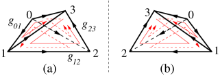
Figure 6: (Color online) Two branched simplices with opposite orientations. (a) A branched simplex with positive orientation and (b) a branched simplex with negative orientation.

Let $M_{\text{tri}}$ be a triangulation of the $d$-dimensional space-time. We will call the triangulation $M_{\text{tri}}$ as a space-time complex, and a cell in the complex as a simplex. In order to define a generic lattice theory on the space-time complex $M_{\text{tri}}$, it is important to give the vertices of each simplex a local order. A nice local scheme to order the vertices is given by a branching structure.Costantino (2005); Chen et al. (2013a, 2012) A branching structure is a choice of orientation of each edge in the $d$-dimensional complex so that there is no oriented loop on any triangle (see Fig. 6).

The branching structure induces a local order of the vertices on each simplex. The first vertex of a simplex is the vertex with no incoming edges, and the second vertex is the vertex with only one incoming edge, etc . So the simplex in Fig. 6a has the following vertex ordering: $0,1,2,3$.

The branching structure also gives the simplex (and its sub simplexes) an orientation denoted by $s_{ij\cdots k}=\pm 1$. Fig. 6 illustrates two $3$-simplices with opposite orientations $s_{0123}=1$ and $s_{0123}=*$. The red arrows indicate the orientations of the $2$-simplices which are the subsimplices of the $3$-simplices. The black arrows on the edges indicate the orientations of the $1$-simplices.

E.2.2 Lattice gauge theory with a global symmetry

To define a lattice gauge theory with a gauge group $GG$ and a global symmetry group $SG$, let $G$ be an extension of $SG$ by $GG$: $G=GG\rightthreetimes SG$. Here we will assume $GG$ to be a finite group.

In our lattice gauge theory, the degrees of freedom on the vertices of the space-time complex, is described by $g_{i}\in G$ where $i$ labels the vertices. The gauge degrees of freedom are on the edges $ij$ which are described by $h_{ij}\in GG$.

The action amplitude $\hskip 1.0pt\mathrm{e}^{-S_{\text{cell}}}$ for a $d$-cell $(ij\cdots k)$ is complex function of $g_{i}$ and $h_{ij}$: $V_{ij\cdots k}(\{h_{ij}\},\{g_{i}\})$. The total action amplitude $\hskip 1.0pt\mathrm{e}^{-S}$ for configuration (or a path) is given by

$$\hskip 1.0pt\mathrm{e}^{-S}=\prod_{(ij\cdots k)}[V_{ij\cdots k}(\{h_{ij}\},\{g_{i}\})]^{s_{ij\cdots k}}$$ (184)

where $\prod_{(ij\cdots k)}$ is the product over all the $d$-cells $(ij\cdots k)$. Note that the contribution from a $d$-cell $(ij\cdots k)$ is $V_{ij\cdots k}(\{h_{ij}\},\{g_{i}\})$ or $V^{*}_{ij\cdots k}(\{h_{ij}\},\{g_{i}\})$ depending on the orientation $s_{ij\cdots k}$ of the cell. Our lattice theory is defined by following imaginary-time path integral (or partition function)

$$Z_{\text{gauge}}=\sum_{\{h_{ij}\},\{g_{i}\}}\prod_{(ij\cdots k)}[V_{ij\cdots k}(\{h_{ij}\},\{g_{i}\})]^{s_{ij\cdots k}}$$ (185)

If the above action amplitude $\prod_{(ij\cdots k)}[V_{ij\cdots k}(\{h_{ij}\},\{g_{i}\})]^{s_{ij\cdots k}}$ on closed space-time complex ($\partial M_{\text{tri}}=\emptyset$) is invariant under the gauge transformation

$$h_{ij}\to g^{\prime}_{ij}=h_{i}h_{ij}h_{j}^{-1},g_{i}\to g^{\prime}_{i}=h_{i}g_{i}\ \ \ h_{i}\in GG$$ (186)

then the action amplitude $V_{ij\cdots k}(\{h_{ij}\},\{g_{i}\})$ defines a gauge theory of gauge group $GG$. If the action amplitude is invariant under the global transformation

$$h_{ij}\to h^{\prime}_{ij}=gh_{ij}g^{-1},g_{i}\to g^{\prime}_{i}=gg_{i}\ \ \ g\in G,$$ (187)

then the action amplitude $V_{ij\cdots k}(\{h_{ij}\},\{g_{i}\})$ defines a $GG$ lattice gauge theory with a global symmetry $SG=G/GG$. (We need to mod out $GG$ since when $h\in GG$, it is a part of gauge transformation which does not change the physical states, instead of a global symmetry transformation which change a physical state to another one.)

However, in this paper, we are mainly considering a system with a global symmetry $G$, where we gauged a subgroup $GG\subset G$. The resulting gauge connection $h_{ij}$ is treated as non-dynamical probe fields. Such a system

Using a cocycle $\nu_{d}(g_{0},g_{1},\cdots,g_{d})\in{\cal H}^{d}(G,\mathbb{R}/\mathbb{Z}),\ g_{i}\in G$ [where $\nu_{d}(g_{0},g_{1},\cdots,g_{d})$ is a real function over $G^{d+1}$], we can construct an action amplitude $V_{ij\cdots k}(\{h_{ij}\},\{g_{i}\})$ that define a gauge theory with gauge group $SG$ and global symmetry $SG$. The gauge theory action amplitude is obtained from $\nu_{d}(g_{0},g_{1},\cdots,g_{d})$ as

$$V_{01\cdots d}(\{h_{ij}\},\{g_{i}\})=0,\text{ if }h_{ij}h_{jk}\neq h_{ik}$$ (188)

$$V_{01\cdots d}(\{h_{ij}\},\{g_{i}\})=\hskip 1.0pt\mathrm{e}^{2\pi\hskip 1.0pt\mathrm{i}\hskip 1.0pt\nu_{d}(h_{0}g_{0},h_{1}g_{1},\cdots,h_{d}g_{d})},$$

$$=\hskip 1.0pt\mathrm{e}^{2\pi\hskip 1.0pt\mathrm{i}\hskip 1.0pt\omega_{d}(g_{0}^{-1}h_{01}g_{1},\cdots,g_{d-1}^{-1}h_{d-1,d}g_{d})},\text{ if }h_{ij}h_{jk}=h_{ik},$$

where $h_{i}$ are given by

$$h_{0} =1, h_{1} =h_{0}h_{01}, h_{2} =h_{1}h_{12}, h_{3} =h_{2}h_{23},\cdots$$ (189)

and $\omega_{d}$ is the nonhomogenous cocycle that corresponds to $\nu_{d}$

$$\omega_{d}(h_{01},h_{12},\cdots,h_{d-1,d})=\nu_{d}(h_{0},h_{1},\cdots,h_{d}).$$ (190)

To see the above action amplitude defines a $GG$ lattice gauge theory with a global symmetry $SG$, we note that the cocycle satisfies the cocycle condition

$$\nu_{d}(g_{0},g_{1},\cdots,g_{d})=\nu_{d}(gg_{0},gg_{1},\cdots,gg_{d})\text{ mod }1,\ \ \ g\in G$$

$$\sum_{i}\nu_{d}(g_{0},\cdots,\hat{g}_{i},\cdots,g_{d+1})=0\text{ mod }1$$ (191)

where $g_{0},\cdots,\hat{g}_{i},\cdots,g_{d+1}$ is the sequence $g_{0},\cdots,g_{i},\cdots,g_{d+1}$ with $g_{i}$ removed. Using such a property, one can check that the above action amplitude $V_{01\cdots d}(\{h_{ij}\},\{g_{i}\})$ is invariant under the global symmetry transformation (187). We can also rewrite the partition function as (see eqn. (188))

$$Z=\sum_{\{h_{ij}\},\{g_{i}\}}\prod_{(ij\cdots k)}[V_{ij\cdots k}(\{g_{i}^{-1}h_{ij}g_{j}\},\{1\})]^{s_{ij\cdots k}}$$ (192)

which is explicitly gauge invariant. Thus it defines a symmetric gauge theory with a gauge group $GG$ and a global symmetry group $SG$.

We note that the action amplitude is non-zero only when $h_{ij}h_{jk}=h_{ik}$ or $h_{ij}h_{jk}h^{-1}_{ik}=1$. The condition $h_{ij}h_{jk}h^{-1}_{ik}\equiv\hskip 1.0pt\mathrm{e}^{\hskip 1.0pt\mathrm{i}\hskip 1.0pt\text{``gauge flux''}}=1$ is the zero-flux condition on the triangle $(ijk)$ or the flat connection condition. The corresponding gauge theory is in the weak-coupling limit (actually is at the zero-coupling). This condition can be implemented precisely only when $GG$ is finite. With the flat connection condition $h_{ij}h_{jk}=h_{ik}$, $h_{i}$’s and the gauge equivalent sets of $h_{ij}$ have an one-to-one correspondence.

Since the total action amplitude $\prod_{(ij\cdots k)}[V_{ij\cdots k}(\{h_{ij}\},\{g_{i}\})]^{s_{ij\cdots k}}$ on a sphere is always equal to 1 if the gauge flux vanishes, therefore $V_{ij\cdots k}(\{h_{ij}\},\{g_{i}\})$ describes a quantized topological term in weak-coupling gauge theory (or zero-coupling gauge theory). This way, we show that a quantized topological term in a weak-coupling gauge theory with gauge group $GG$ and symmetry group $SG$ can be constructed from each element of ${\cal H}^{d}(G,\mathbb{R}/\mathbb{Z})$.

Figure 7: Each time-step of evolution is given by the path integral on a particular form of branched graph. Here is an example in 1+1D. In SPT states, the gauge connection $h_{ij}$ on the links is a non-dynamical probe field. In this case, the gauge connection $h_{ij}=1$ on the time-links (i.e. the vertical links). In SET states, the gauge connection $h_{ij}$ on the links is a dynamical field. In this case, the gauge connection $h_{ij}$ can be non-trivial on any links.

Figure 8: The reduction of double-layer time-step to single-layer time-step on space with boundary in an 1+1D example.

E.2.3 From path integral to Hamiltonian

A path integral can give us an amplitude $Z[\{g_{i}^{\prime},h_{ij}^{\prime}\},\{g_{i},h_{ij}\}]$ for a configuration $\{g_{i},h_{ij}\}$ at $t$ to another configuration $\{g_{i}^{\prime},h_{ij}^{\prime}\}$ at $t^{\prime}$. We like to interpret $Z[\{g_{i}^{\prime},h_{ij}^{\prime}\},\{g_{i},h_{ij}\}]$ as the amplitude of an evolution in imaginary time by a Hamiltonian:

$$Z[\{g_{i}^{\prime},h_{ij}^{\prime}\},\{g_{i},h_{ij}\}]=\langle g_{i}^{\prime},h_{ij}^{\prime}|\hskip 1.0pt\mathrm{e}^{-(t^{\prime}-t)H}|g_{i},h_{ij}\rangle.$$ (193)

However, such an interpretation may not be valid since $Z[\{g_{i}^{\prime},h_{ij}^{\prime}\},\{g_{i},h_{ij}\}]$ may not give raise to a Hermitian matrix. It is a worrisome realization that path integral and Hamiltonian evolution may not be directly related.

Here we would like to use the fact that the path integral that we are considering are defined on the branched graphs with a “reflection” property (see (184)). We like to show that such path integral are better related Hamiltonian evolution. The key is to require that each time-step of evolution is given by branched graphs of the form in Fig. 7. One can show that $Z[\{g_{i}^{\prime},h_{ij}^{\prime}\},\{g_{i},h_{ij}\}]$ obtained by summing over all in the internal indices in the branched graphs Fig. 7 has a form

$$\ \ \ \ Z[\{g_{i}^{\prime},h_{ij}^{\prime}\},\{g_{i},h_{ij}\}]$$ (194)

$$=\sum_{\{g_{i}^{\prime\prime},h_{ij}^{\prime\prime}\}}U^{*}[\{g_{i}^{\prime\prime},h_{ij}^{\prime\prime}\},\{g_{i}^{\prime},h_{ij}^{\prime}\}]\ U[\{g_{i}^{\prime\prime},h_{ij}^{\prime\prime}\},\{g_{i},h_{ij}\}]$$

and represents a positive-definite Hermitian matrix. Thus the path integral of the form (184) always correspond to a Hamiltonian evolution in imaginary time. In fact, the above $Z[\{g_{i}^{\prime},h_{ij}^{\prime}\},\{g_{i},h_{ij}\}]$ can be viewed as an imaginary-time evolution $T=\hskip 1.0pt\mathrm{e}^{-\Delta\tau H}$ for a single time step.

For most cases studied in this paper, $h_{ij}$ is a static probe field. In those case, $h_{ij}$ are the same on all the time slices and $h_{ij}=1$ on the vertical time links. In this case, $Z[\{g_{i}^{\prime},h_{ij}\},\{g_{i},h_{ij}\}]$ (with fixed $h_{ij}$) can still be viewed as an imaginary-time evolution $T=\hskip 1.0pt\mathrm{e}^{-\Delta\tau H}$ for a single time step, where only $g_{i}$’s are dynamical.

For the ideal path integrals with the action-amplitudes described by the cocycles, we can reduce the double-layer time-step to a single-layer time-step, using the retriangulation invariance of the action-amplitudes if the space has no boundary. If the space does have boundary, we can still reduce the double-layer time-step to a single-layer time-step, but with some extra terms on the boundary (see Fig. 8).

Appendix F Physical properties of defects in 2+1D $Z_{n}$ SPT states

If we view $h_{ij}$ in the last section as a static probe field, then the formalism developed in the last section can be viewed as the path integral description of SPT states with possible monodromy defects or other possible twists described the “gauge configuration” $h_{ij}$ on the links. In this section, we are going to use such a formalism to study the physical properties of defects in SPT states.

F.1 Symmetry transformations and their non-factorization

First let us examine how symmetry transformations act on the defects. Consider a system with symmetry $G$. The evolution operator $T=\hskip 1.0pt\mathrm{e}^{-\tau H}$ satisfies

$$W_{g}TW_{g}^{-1}=T,\ \ \ \ g\in G$$ (195)

where $W_{g}$ is a represent of the symmetry. We like to examine the amplitude of the evolution from a configuration $\{g_{i},h_{ij}\}$ to its symmetry $g$ transformed configuration $\{gg_{i},h_{ij}\}$ (where we have assumed that $gh_{ij}g^{-1}=h_{ij}$.) Or more precisely, we want to examine the trace ${\rm Tr}(T^{N}W_{g})$. Such a trace can be expressed as a graph which is periodic in time direction, with one layer of vertical time links given by $h_{ij}=g$, while other layers of vertical time links by $h_{ij}=1$ (see Fig. 9).

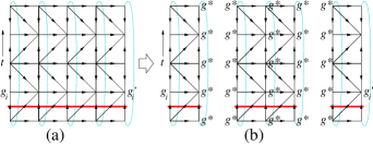
Figure 9: (a) The trace ${\rm Tr}(T^{N}W_{g})$ can be represented by a graph which is periodic in time direction, with one layer of vertical time links with $h_{ij}=g$, in an 1+1D example. Those vertical time links are marked by red-line crossing them. (a $\to$ b) We can use the retriangulation invariance of the action-amplitudes to set all the internal $g_{i}$ to a fixed $g^{*}$ without changing the action-amplitude. (b) For fixed $g^{*}$, we can rewrite one graph as three graphs, where the middle graph just represents a phase factor.

For the ideal path integrals with the action-amplitudes described by the cocycles, the action-amplitudes only depend on the $g_{i}$’s on the boundary. (Here we assume that $h_{ij}$’s are fixed non-dynamical probe fields. We can use the retriangulation invariance of the action-amplitudes to set all the internal $g_{i}$ to a fixed $g^{*}$ without changing the action-amplitude. (Usually, we may take $g^{*}=1$.) Thus the trace ${\rm Tr}(T^{N}W_{g})$ can be represented by the three graphs in Fig. 9(b). We see that the trace ${\rm Tr}(T^{N}W_{g})$ factorizes into independent boundary terms (one for each boundary) and the non-dynamical bulk phase factor:

$${\rm Tr}(T^{N}W_{g})=$$ (196)

$${\rm Tr}U^{\text{bulk}}_{g}{\rm Tr}(T_{\text{bndry,1}}^{N}W^{\text{bndry,1}}_{g}){\rm Tr}(T_{\text{bndry,2}}^{N}W^{\text{bndry,2}}_{g})$$

Note that $U^{\text{bulk}}_{g}$ is $1\times 1$ matrix described by the middle graph in Fig. 9(b). In fact $U^{\text{bulk}}_{g}$ is a pure phase factor. $T_{\text{bndry,1}}^{N}$ and $T_{\text{bndry,2}}^{N}$ describe the dynamic time evolution on the two boundaries, which are independent of each other. We see that to total symmetry transformation $W_{g}$ has a form

$$W_{g}=U^{\text{bulk}}_{g}\ W^{\text{bndry,1}}_{g}\otimes W^{\text{bndry,2}}_{g}$$ (197)

If the phase factor $U^{\text{bulk}}_{g}=1$, then the total symmetry transformation factorize on the two independent boundaries. However, if $U^{\text{bulk}}_{g}$ form a non-trivial 1D representation of $G$, the total $G$ quantum number will the sum of the $G$ quantum numbers on each boundaries plus a shift generated by $U^{\text{bulk}}_{g}$. In this case, the total symmetry transformations do not cleanly factorize into independent boundary terms. It contains an extra phase factor $U^{\text{bulk}}_{g}$.

F.2 The low energy effective theory and low energy effective symmetry at the monodromy defects

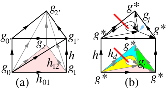
Figure 10: (Color online) (a) The action amplitude on the complex in (a), for an ideal fixed point action, is given by $C(g_{0},g_{1},g_{2};g_{0^{\prime}},g_{1^{\prime}},g_{2^{\prime}};h_{01},h_{02},h)$. The complex is formed by three tetrahedrons: $(0122^{\prime})$, $(00^{\prime}1^{\prime}2^{\prime})$, and $(011^{\prime}2^{\prime})$. The triangles $(012)$ and $(0^{\prime}1^{\prime}2^{\prime})$ are on two time slices. (b) A defect is described by the dynamical variables $g_{i},g_{j}$. When $h_{kl}$ on the links crossed by the red lines are non-trivial ($h_{kl}=h_{d}\neq 1$), the defect is a monodromy defect. When $h=g$ on the vertical links (the time links), it describes the insertion $W_{g}$ in the path integral. Note that $g_{i},g_{j}$ are surrounded by $g^{*}$’s and the complex (b) is formed by four complices of the type in (a), represented by the four colors of the base triangles.

In this section, we are going to apply the formalism developed in the last section to study the low energy effective theory and low energy effective symmetry at the monodromy defects in 2+1D $Z_{n}$ SPT states. The monodromy defects are created by a $h_{d}$ twist ($h_{d}\in Z_{n}$).

A $Z_{n}$ monodromy defect is described by Fig. 10(b). The low energy degrees of freedom in the defect are described by $g\in Z_{n}$. Let us use $g^{(k)}=\hskip 1.0pt\mathrm{e}^{\frac{2\pi k\hskip 1.0pt\mathrm{i}\hskip 1.0pt}{n}},\ \ k=0,\cdots,n-1$, to describe the $Z_{n}$ group elements. The states on a defect are described by $|g^{(k)}\rangle$. To construct the path integral eqn. (196) that describes low energy dynamics of the defects, let us first introduce

$$\ \ \ \ C(g_{0},g_{1},g_{2};g_{0^{\prime}},g_{1^{\prime}},g_{2^{\prime}};h_{01},h_{02},h)$$

$$=\hskip 1.0pt\mathrm{e}^{2\pi\hskip 1.0pt\mathrm{i}\hskip 1.0pt\omega_{3}(g_{0}^{-1}h_{01}g_{1},g_{1}^{-1}h_{12}g_{2},g_{2}^{-1}hg_{2^{\prime}})}\times$$

$$\ \ \ \ \hskip 1.0pt\mathrm{e}^{-2\pi\hskip 1.0pt\mathrm{i}\hskip 1.0pt\omega_{3}(g_{0}^{-1}h_{01}g_{1},g_{1}^{-1}hg_{1^{\prime}},g_{1^{\prime}}^{-1}h_{12}g_{2^{\prime}})}\times$$

$$\ \ \ \ \hskip 1.0pt\mathrm{e}^{2\pi\hskip 1.0pt\mathrm{i}\hskip 1.0pt\omega_{3}(g_{0}^{-1}hg_{0^{\prime}},g_{0^{\prime}}^{-1}h_{01}g_{1^{\prime}},g_{1^{\prime}}^{-1}h_{12}g_{2^{\prime}})}.$$ (198)

Physically, the above is the action amplitude for ideal fixed point system described by (188), on the complex in Fig. 10(a). Using $C(g_{0},g_{1},g_{2},g_{0^{\prime}},g_{2^{\prime}},g_{2^{\prime}},h_{01},h_{02},h)$, we can construct a $|G|\times|G|$ matrix $U_{\text{def}}(g^{*},h_{d},h)$ whose matrix elements are given by

$$[U_{\text{def}}(g^{*},h_{d},h)]_{g_{j},g_{i}}=\frac{C(g_{i},g^{*},g^{*};g_{j},g^{*},g^{*};1,1,h)}{C(g^{*},g_{i},g^{*};g^{*},g_{j},g^{*};1,1,h)}\times$$

$$C(g^{*},g_{i},g_{i};g^{*},g_{j},g_{j};1,h_{d},h)C(g^{*},g_{i},g^{*};g^{*},g_{j},g^{*};h_{d},1,h).$$ (199)

Then the $|G|\times|G|$ matrix $T^{\Delta\tau}_{\text{def}}(g^{*},h_{d})$

$$T^{\Delta\tau}_{\text{def}}(g^{*},h_{d})=[U_{\text{def}}(g^{*},h_{d},1)]^{\dagger}U_{\text{def}}(g^{*},h_{d},1)$$ (200)

will generate the imaginary-time evolution for a single defect. We have (for two defects)

$${\rm Tr}(T^{N})=U_{0}^{\text{bulk}}{\rm Tr}[T^{\Delta\tau}_{\text{def}}(g^{*},h_{d})]^{N}{\rm Tr}[T^{\Delta\tau}_{\text{def}}(g^{*},h_{d})]^{N},$$ (201)

where $T$ is the imaginary-time evolution operator $\hskip 1.0pt\mathrm{e}^{-\Delta\tau H}$ of the whole system for a single time step, $T^{\Delta\tau}_{\text{def}}$ is the imaginary-time evolution operator for a single defect, and the bulk contribution $U^{\text{bulk}}=1$.

Let us calculate $T^{\Delta\tau}_{\text{def}}(g^{*},h_{d})$ for the monodromy defects in the 2+1D $Z_{n}$ SPT state. We will always choose $g^{*}=1$. The cocycles in ${\cal H}^{3}(Z_{n},\mathbb{R}/\mathbb{Z})$ are labeled by $m=0,1,\cdots,n-1$, and are given by

$$\omega_{3}(g^{(k_{1})},g^{(k_{2})},g^{(k_{3})}) =\hskip 1.0pt\mathrm{e}^{m\frac{2\pi\hskip 1.0pt\mathrm{i}\hskip 1.0pt}{n^{2}}k_{1}(k_{2}+k_{3}-[k_{2}+k_{3}]_{n})},$$

$$g^{(k)} =\hskip 1.0pt\mathrm{e}^{\frac{2\pi k\hskip 1.0pt\mathrm{i}\hskip 1.0pt}{n}},$$ (202)

where $[k]_{n}$ is a short-hand notation for

$$[k]_{n}\equiv\text{mod}(k,n).$$ (203)

In the following, we will only consider the $Z_{n}$ SPT phases described by $m=1$.

Let us first concentrate on 2+1D $Z_{2}$ SPT states. Using the cocycles, we find that, for a 2+1D $Z_{2}$ SPT state,

$$U_{\text{def}}(g^{*},h_{d}=1,h=1) =\begin{pmatrix}1&1\\ 1&1\\ \end{pmatrix}$$

$$T^{\Delta\tau}_{\text{def}}(g^{*},h_{d}=1) =\begin{pmatrix}2&2\\ 2&2\\ \end{pmatrix}.$$ (204)

We find that for a trivial monodromy defect, the ground state on a defect is given by $|g=1\rangle+|g=-1\rangle$, which is an expected result. We also find that

$$U_{\text{def}}(g^{*},h_{d}=-1,h=1) =\begin{pmatrix}1&1\\ -1&1\\ \end{pmatrix}$$

$$T^{\Delta\tau}_{\text{def}}(g^{*},h_{d}=-1) =\begin{pmatrix}2&0\\ 0&2\\ \end{pmatrix}.$$ (205)

This mean that the a non-trivial monodromy defect carry two degenerate states $g=|\pm 1\rangle$. However, the degeneracy can be lifted by perturbations that respect the symmetry.

To study the $Z_{2}$ symmetry of the defects, let us consider the path integral

$${\rm Tr}(W_{g}T^{N})=U_{g}^{\text{bulk}}U_{0}^{\text{bulk}}\times$$ (206)

$$\ \ {\rm Tr}(W^{\text{def}}_{g}[T^{\Delta\tau}_{\text{def}}(g^{*},h_{d})]^{N}){\rm Tr}(W^{\text{def}}_{g}[T^{\Delta\tau}_{\text{def}}(g^{*},h_{d})]^{N}),$$

where $W_{g},\ \ g\in Z_{2}$ is a representation of $Z_{2}$ acting on the total system: $|\{g_{k}\}\rangle\to|\{gg_{k}\}\rangle$, and $W^{\text{def}}_{g}$ describes how $Z_{2}$ symmetry transformation act on the low energy degrees of freedom on the defect. We note that now the phase factor contribution from the bulk $U_{g}^{\text{bulk}}U_{0}^{\text{bulk}}$ has a $g$ dependence, and thus becomes non-trivial.

Let us first calculate $W^{\text{def}}_{g}$. Note that ${\rm Tr}[T^{\Delta\tau}_{\text{def}}(g^{*},h_{d})]^{N}$ is a trace of product of many $U_{\text{def}}(g^{*},h_{d},h=1)$ operators. To calculate ${\rm Tr}W^{\text{def}}_{g}[T^{\Delta\tau}_{\text{def}}(g^{*},h_{d})]^{N}$, we just need to replace one of the $U_{\text{def}}(g^{*},h_{d},h=1)$’s by $U_{\text{def}}(g^{*},h_{d},h=g)$. Therefore, we have

$$\ \ \ \ [U_{\text{def}}(g^{*},h_{d},1)]^{\dagger}U_{\text{def}}(g^{*},h_{d},g)$$

$$=[U_{\text{def}}(g^{*},h_{d},1)]^{\dagger}U_{\text{def}}(g^{*},h_{d},1)W^{\text{def}}_{g}.$$ (207)

For $Z_{2}$ SPT state, we find

$$U_{\text{def}}(g^{*},h_{d}=-1,h=1) =\begin{pmatrix}1&1\\ -1&1\\ \end{pmatrix},$$

$$U_{\text{def}}(g^{*},h_{d}=-1,h=-1) =\begin{pmatrix}1&-1\\ 1&1\\ \end{pmatrix}.$$ (208)

Eqn. F.2 becomes (for $h_{d}=-1$)

$$\begin{pmatrix}0&-2\\ 2&0\\ \end{pmatrix}=\begin{pmatrix}2&0\\ 0&2\\ \end{pmatrix}W^{\text{def}}_{-1}.$$ (209)

We find that

$$W^{\text{def}}_{-1}=\begin{pmatrix}0&-1\\ 1&0\\ \end{pmatrix}=\hskip 1.0pt\mathrm{i}\hskip 1.0pt\sigma^{2},$$ (210)

for a non-trivial monodromy defect.

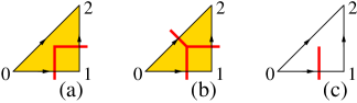
Figure 11: (Color online) A graphic representation of $U(-1,h_{01},h_{12})$. The edges crossed by the red line have $h_{ij}=-1$. The edges not crossed by the red line have $h_{ij}=1$. The gauge configurations in (a) and (b) have $U(-1,h_{01},h_{12})=-1$. The gauge configuration in (c) and other configurations have $U(-1,h_{01},h_{12})=1$.

Next, let us calculate the phase factor from the bulk, $U_{g}^{\text{bulk}}$. For this purpose, we introduce

$$U(g,h_{01},h_{12}) =\frac{\hskip 1.0pt\mathrm{e}^{\hskip 1.0pt\mathrm{i}\hskip 1.0pt2\pi\omega_{3}(h_{01},h_{12},h_{22^{\prime}})}\hskip 1.0pt\mathrm{e}^{\hskip 1.0pt\mathrm{i}\hskip 1.0pt2\pi\omega_{3}(h_{00^{\prime}},h_{0^{\prime}1^{\prime}},h_{1^{\prime}2^{\prime}})}}{\hskip 1.0pt\mathrm{e}^{\hskip 1.0pt\mathrm{i}\hskip 1.0pt2\pi\omega_{3}(h_{01},h_{11^{\prime}},h_{1^{\prime}2^{\prime}})}}$$

$$=C(g^{*},g^{*},g^{*};g^{*},g^{*},g^{*};h_{01},h_{12},g)$$ (211)

which is the action-amplitude on a single space-time complex in Fig. 10(a) with $g_{i}=g_{i^{\prime}}=g^{*}=1$. We find that (see Fig. 11)

$$U(-1,-1,-1) =-1,$$

$$U(g,h_{01},h_{12}) =1\text{ otherwise}.$$ (212)

The total action-amplitude for the bulk is given by

$$U^{\text{bulk}}_{g}={\prod_{(ijk)}}^{\prime}U^{s_{ijk}}(g,h_{01},h_{12})/U^{s_{ijk}}(1,h_{01},h_{12}),$$ (213)

where $s_{ijk}$ describes the orientation of the triangle $(ijk)$, and $\prod^{\prime}_{(ijk)}$ is a product over all the triangles that are not monodromy defects (i.e. contain no $Z_{2}$-flux). From Fig. 3, we see that $U^{\text{bulk}}_{-1}=-1$ for two identical monodromy defects. Therefore, the low energy effective $Z_{2}$ symmetry transformation $W_{g}$ is given by

$$W_{g}=U^{\text{bulk}}_{g}W^{\text{def}}_{g}\otimes W^{\text{def}}_{g}$$ (214)

For $g=-1$, we have

$$W_{-1}=U^{\text{bulk}}_{-1}W^{\text{def}}_{-1}\otimes W^{\text{def}}_{-1}=-\hskip 1.0pt\mathrm{i}\hskip 1.0pt\sigma^{2}\otimes\hskip 1.0pt\mathrm{i}\hskip 1.0pt\sigma^{2},$$ (215)

where the first $\hskip 1.0pt\mathrm{i}\hskip 1.0pt\sigma^{2}$ acts on the states on the first monodromy defect and the second $\hskip 1.0pt\mathrm{i}\hskip 1.0pt\sigma^{2}$ on the second monodromy defect.

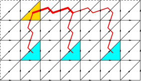
Figure 12: (Color online) A $Z_{3}$-gauge configuration with three identical $Z_{3}$ monodromy defects (blue triangles) on a torus. The details of a monodromy defect are given in Fig. 10(b). The yellow triangle contributes a phase factor $\hskip 1.0pt\mathrm{e}^{2\pi\hskip 1.0pt\mathrm{i}\hskip 1.0pt/3}$ to $U^{\text{bulk}}_{g^{(1)}}$.

The above calculation can be generalized to $n$ identical monodromy defects in a 2+1D $Z_{n}$ SPT state, described by the cocycle eqn. (F.2). We find that the low energy effective $Z_{n}$ symmetry transformation $W_{g}$ is given by

$$W_{g^{(1)}} =U^{\text{bulk}}_{g^{(1)}}\underbrace{W^{\text{def}}_{g^{(1)}}\otimes\cdots\otimes W^{\text{def}}_{g^{(1)}}}_{n\text{ terms}},$$

$$g^{(k)} =\hskip 1.0pt\mathrm{e}^{2\pi k\hskip 1.0pt\mathrm{i}\hskip 1.0pt/n},$$ (216)

Here $W^{\text{def}}_{g^{(1)}}$ is a $n\times n$ matrix acting on the states on one $Z_{n}$ monodromy defect. If we choose $|g^{(k)}\rangle$ to be the basis of the states on one $Z_{n}$ monodromy defect, the action of $W^{\text{def}}_{g^{(1)}}$ is given by

$$W^{\text{def}}_{g^{(1)}})|g^{(k)}\rangle =f_{k}|g^{(1)}g^{(k)}\rangle,\ \ \ k=0,1,\cdots,n-1,$$

$$f_{0} =\hskip 1.0pt\mathrm{e}^{2\pi\hskip 1.0pt\mathrm{i}\hskip 1.0pt/n},\ \ \ \ \ f_{k>0}=1.$$ (217)

$U^{\text{bulk}}_{g}$ is a pure phase factor which is given by eqn. (213). For the $Z_{n}$ SPT state described by the cocycle eqn. (F.2), we find that

$$U(g^{(1)},h_{01}^{(k)},h_{12}^{(k^{\prime})}) =\hskip 1.0pt\mathrm{e}^{2\pi\hskip 1.0pt\mathrm{i}\hskip 1.0pt(k+k^{\prime}-[k+k^{\prime}]_{n})/n^{2}},$$

$$k,k^{\prime} =0,1,\cdots,n-1.$$ (218)

This gives us (see Fig. 12)

$$U^{\text{bulk}}_{g^{(1)}}=\prod_{k=0}^{n-1}\hskip 1.0pt\mathrm{e}^{2\pi\hskip 1.0pt\mathrm{i}\hskip 1.0pt(k+1-[k+1]_{n})/n^{2}}=\hskip 1.0pt\mathrm{e}^{2\pi\hskip 1.0pt\mathrm{i}\hskip 1.0pt/n}$$ (219)

We note that $(W^{\text{def}}_{g^{(1)}})^{n}=\hskip 1.0pt\mathrm{e}^{2\pi\hskip 1.0pt\mathrm{i}\hskip 1.0pt/n}$. So we may say that each monodromy defect carries $\frac{1}{n}+$integer $Z_{n}$ charges. The fact that $U^{\text{bulk}}_{g^{(1)}}=\hskip 1.0pt\mathrm{e}^{2\pi\hskip 1.0pt\mathrm{i}\hskip 1.0pt/n}$ implies that the bulk also carries an $Z_{n}$-charge 1. So

SPT invariant 40:

$n$ identical elementary monodromy defects (i.e. generated by the twist $h_{d}=g^{(1)}$) in 2+1D $Z_{n}$ SPT states on a torus always carry a total $Z_{n}$-charge 2, if the $Z_{n}$ SPT states are described by the $m=1$ cocycle in ${\cal H}^{3}(Z_{n},\mathbb{R}/\mathbb{Z})$ (see eqn. (F.2)).

Although we only present the derivation of the above result for a particular choice of cocycles as in eqn. (F.2), we have checked that the result remains to be valid for any choices of cocycles. In other words, the above result does not change if we add a coboundary to the cocycle that describes the SPT state.

There is a simple way to understand the SPT invariant 40. We may view the $Z_{n}$ SPT state as a $U(1)$ SPT state with Hall conductance $\sigma_{xy}=2\frac{1}{2\pi}$ in 2+1D. An $Z_{n}$ monodromy defect corresponds to $2\pi/n$ $U(1)$ flux which will nuclear $2\frac{1}{n}$ $U(1)$ charge. $2\frac{1}{n}$ $U(1)$ charge correspond to $2\frac{1}{n}$ $Z_{n}$ charge. Thus $n$ identical $Z_{n}$ monodromy defects carry a total $Z_{n}$ charge $2$.

References

• Landau (1937) L. D. Landau, Phys. Z. Sowjetunion 11, 26 (1937).
• Ginzburg and Landau (1950) V. L. Ginzburg and L. D. Landau, Zh. Eksp. Teor. Fiz. 20, 1064 (1950).
• Landau and Lifschitz (1958) L. D. Landau and E. M. Lifschitz, Statistical Physics - Course of Theoretical Physics Vol 5 (Pergamon, London, 1958).
• Kalmeyer and Laughlin (1987) V. Kalmeyer and R. B. Laughlin, Phys. Rev. Lett. 59, 2095 (1987).
• Wen et al. (1989) X.-G. Wen, F. Wilczek, and A. Zee, Phys. Rev. B 39, 11413 (1989).
• Wen (1989) X.-G. Wen, Phys. Rev. B 40, 7387 (1989).
• Wen and Niu (1990) X.-G. Wen and Q. Niu, Phys. Rev. B 41, 9377 (1990).
• Wen (1990) X.-G. Wen, Int. J. Mod. Phys. B 4, 239 (1990).
• Keski-Vakkuri and Wen (1993) E. Keski-Vakkuri and X.-G. Wen, Int. J. Mod. Phys. B 7, 4227 (1993).
• Levin and Wen (2006) M. Levin and X.-G. Wen, Phys. Rev. Lett. 96, 110405 (2006), eprint cond-mat/0510613.
• Kitaev and Preskill (2006) A. Kitaev and J. Preskill, Phys. Rev. Lett. 96, 110404 (2006).
• Chen et al. (2010) X. Chen, Z.-C. Gu, and X.-G. Wen, Phys. Rev. B 82, 155138 (2010), eprint arXiv:1004.3835.
• Levin and Wen (2005) M. Levin and X.-G. Wen, Phys. Rev. B 71, 045110 (2005), eprint cond-mat/0404617.
• Verstraete et al. (2005) F. Verstraete, J. I. Cirac, J. I. Latorre, E. Rico, and M. M. Wolf, Phys. Rev. Lett. 94, 140601 (2005).
• Vidal (2007) G. Vidal, Phys. Rev. Lett. 99, 220405 (2007).
• Tsui et al. (1982) D. C. Tsui, H. L. Stormer, and A. C. Gossard, Phys. Rev. Lett. 48, 1559 (1982).
• Laughlin (1983) R. B. Laughlin, Phys. Rev. Lett. 50, 1395 (1983).
• Read and Sachdev (1991) N. Read and S. Sachdev, Phys. Rev. Lett. 66, 1773 (1991).
• Wen (1991a) X.-G. Wen, Phys. Rev. B 44, 2664 (1991a).
• Moessner and Sondhi (2001) R. Moessner and S. L. Sondhi, Phys. Rev. Lett. 86, 1881 (2001).
• Moore and Read (1991) G. Moore and N. Read, Nucl. Phys. B 360, 362 (1991).
• Wen (1991b) X.-G. Wen, Phys. Rev. Lett. 66, 802 (1991b).
• Willett et al. (1987) R. Willett, J. P. Eisenstein, H. L. Strörmer, D. C. Tsui, A. C. Gossard, and J. H. English, Phys. Rev. Lett. 59, 1776 (1987).
• Radu et al. (2008) I. P. Radu, J. B. Miller, C. M. Marcus, M. A. Kastner, L. N. Pfeiffer, and K. W. West, Science 320, 899 (2008).
• Freedman et al. (2004) M. Freedman, C. Nayak, K. Shtengel, K. Walker, and Z. Wang, Ann. Phys. (NY) 310, 428 (2004), eprint cond-mat/0307511.
• Gu et al. (2010) Z.-C. Gu, Z. Wang, and X.-G. Wen (2010), eprint arXiv:1010.1517.
• Lu et al. (2010) Y.-M. Lu, X.-G. Wen, Z. Wang, and Z. Wang, Phys. Rev. B 81, 115124 (2010), eprint arXiv:0910.3988.
• Blok and Wen (1990) B. Blok and X.-G. Wen, Phys. Rev. B 42, 8145 (1990).
• Read (1990) N. Read, Phys. Rev. Lett. 65, 1502 (1990).
• Fröhlich and Kerler (1991) J. Fröhlich and T. Kerler, Nucl. Phys. B 354, 369 (1991).
• Wen and Zee (1992) X.-G. Wen and A. Zee, Phys. Rev. B 46, 2290 (1992).
• Belov and Moore (2005) D. Belov and G. W. Moore (2005), eprint arXiv:hep-th/0505235.
• Kapustin and Saulina (2011) A. Kapustin and N. Saulina, Nucl. Phys. B 845, 393 (2011), eprint arXiv:1008.0654.
• Haldane (1983) F. D. M. Haldane, Physics Letters A 93, 464 (1983).
• Affleck et al. (1988) I. Affleck, T. Kennedy, E. H. Lieb, and H. Tasaki, Commun. Math. Phys. 115, 477 (1988).
• Gu and Wen (2009) Z.-C. Gu and X.-G. Wen, Phys. Rev. B 80, 155131 (2009), eprint arXiv:0903.1069.
• Pollmann et al. (2012) F. Pollmann, E. Berg, A. M. Turner, and M. Oshikawa, Phys. Rev. B 85, 075125 (2012), eprint arXiv:0909.4059.
• Kane and Mele (2005a) C. L. Kane and E. J. Mele, Phys. Rev. Lett. 95, 226801 (2005a), eprint cond-mat/0411737.
• Bernevig and Zhang (2006) B. A. Bernevig and S.-C. Zhang, Phys. Rev. Lett. 96, 106802 (2006).
• Kane and Mele (2005b) C. L. Kane and E. J. Mele, Phys. Rev. Lett. 95, 146802 (2005b), eprint cond-mat/0506581.
• Moore and Balents (2007) J. E. Moore and L. Balents, Phys. Rev. B 75, 121306 (2007), eprint cond-mat/0607314.
• Fu et al. (2007) L. Fu, C. L. Kane, and E. J. Mele, Phys. Rev. Lett. 98, 106803 (2007), eprint cond-mat/0607699.
• Qi et al. (2008) X.-L. Qi, T. Hughes, and S.-C. Zhang, Phys. Rev. B 78, 195424 (2008), eprint arXiv:0802.3537.
• Chen et al. (2011a) X. Chen, Z.-C. Gu, and X.-G. Wen, Phys. Rev. B 83, 035107 (2011a), eprint arXiv:1008.3745.
• Schuch et al. (2011) N. Schuch, D. Perez-Garcia, and I. Cirac, Phys. Rev. B 84, 165139 (2011), eprint arXiv:1010.3732.
• Chen et al. (2011b) X. Chen, Z.-C. Gu, and X.-G. Wen, Phys. Rev. B 84, 235128 (2011b), eprint arXiv:1103.3323.
• Chen et al. (2011c) X. Chen, Z.-X. Liu, and X.-G. Wen, Phys. Rev. B 84, 235141 (2011c), eprint arXiv:1106.4752.
• Chen et al. (2013a) X. Chen, Z.-C. Gu, Z.-X. Liu, and X.-G. Wen, Phys. Rev. B 87, 155114 (2013a), eprint arXiv:1106.4772.
• Chen et al. (2012) X. Chen, Z.-C. Gu, Z.-X. Liu, and X.-G. Wen, Science 338, 1604 (2012), eprint arXiv:1301.0861.
• Levin and Stern (2009) M. Levin and A. Stern, Phys. Rev. Lett. 103, 196803 (2009), eprint arXiv:0906.2769.
• Lu and Vishwanath (2012) Y.-M. Lu and A. Vishwanath, Phys. Rev. B 86, 125119 (2012), eprint arXiv:1205.3156.
• Liu and Wen (2013) Z.-X. Liu and X.-G. Wen, Phys. Rev. Lett. 110, 067205 (2013), eprint arXiv:1205.7024.
• Chen and Wen (2012) X. Chen and X.-G. Wen, Phys. Rev. B 86, 235135 (2012), eprint arXiv:1206.3117.
• Hung and Wen (2012) L.-Y. Hung and X.-G. Wen (2012), eprint arXiv:1211.2767.
• Hung and Wan (2012) L.-Y. Hung and Y. Wan, Phys. Rev. B 86, 235132 (2012), eprint arXiv:1207.6169.
• Vishwanath and Senthil (2013) A. Vishwanath and T. Senthil, Phys. Rev. X 3, 011016 (2013), eprint arXiv:1209.3058.
• Xu (2013) C. Xu, Phys. Rev. B 87, 144421 (2013), eprint arXiv:1209.4399.
• Lu and Lee (2012a) Y.-M. Lu and D.-H. Lee (2012a), eprint arXiv:1210.0909.
• Hung and Wen (2013) L.-Y. Hung and X.-G. Wen, Phys. Rev. B 87, 165107 (2013), eprint arXiv:1212.1827.
• Lu and Lee (2012b) Y.-M. Lu and D.-H. Lee (2012b), eprint arXiv:1212.0863.
• Ye and Wen (2013a) P. Ye and X.-G. Wen, Phys. Rev. B 87, 195128 (2013a), eprint arXiv:1212.2121.
• Oon et al. (2012) J. Oon, G. Y. Cho, and C. Xu (2012), eprint arXiv:1212.1726.
• Xu and Senthil (2013) C. Xu and T. Senthil (2013), eprint arXiv:1301.6172.
• Wang and Senthil (2013) C. Wang and T. Senthil (2013), eprint arXiv:1302.6234.
• Burnell et al. (2013) F. J. Burnell, X. Chen, L. Fidkowski, and A. Vishwanath (2013), eprint arXiv:1302.7072.
• Cheng and Gu (2013) M. Cheng and Z.-C. Gu (2013), eprint arXiv:1302.4803.
• Chen et al. (2013b) X. Chen, F. Wang, Y.-M. Lu, and D.-H. Lee (2013b), eprint arXiv:1302.3121.
• Chen et al. (2013c) X. Chen, Y.-M. Lu, and A. Vishwanath (2013c), eprint arXiv:1303.4301.
• Ye and Wen (2013b) P. Ye and X.-G. Wen (2013b), eprint arXiv:1303.3572.
• Metlitski et al. (2013) M. A. Metlitski, C. L. Kane, and M. P. A. Fisher (2013), eprint arXiv:1302.6535.
• Gu and Levin (2013) Z.-C. Gu and M. Levin (2013), eprint arXiv:1304.4569.
• Lu and Vishwanath (2013) Y.-M. Lu and A. Vishwanath (2013), eprint arXiv:1302.2634.
• Levin and Gu (2012) M. Levin and Z.-C. Gu, Phys. Rev. B 86, 115109 (2012), eprint arXiv:1202.3120.
• Wen (1992) X.-G. Wen, Int. J. Mod. Phys. B 6, 1711 (1992).
• Wang and Wen (2012) J. Wang and X.-G. Wen (2012), eprint arXiv:1212.4863.
• Levin (2013) M. Levin (2013), eprint arXiv:1301.7355.
• Gu and Wen (2012) Z.-C. Gu and X.-G. Wen (2012), eprint arXiv:1201.2648.
• Wen (2002) X.-G. Wen, Phys. Rev. B 65, 165113 (2002), eprint cond-mat/0107071.
• Wen (2003) X.-G. Wen, Phys. Rev. D 68, 065003 (2003), eprint hep-th/0302201.
• Wang and Vishwanath (2006) F. Wang and A. Vishwanath, Phys. Rev. B 74, 174423 (2006), eprint arXiv:cond-mat/0608129.
• Essin and Hermele (2013) A. M. Essin and M. Hermele, Phys. Rev. B 87, 104406 (2013), eprint arXiv:1212.0593.
• Mesaros and Ran (2013) A. Mesaros and Y. Ran, Phys. Rev. B 87, 155115 (2013), eprint arXiv:1212.0835.
• Kou et al. (2008) S.-P. Kou, M. Levin, and X.-G. Wen, Phys. Rev. B 78, 155134 (2008), eprint arXiv:0803.2300.
• Kou and Wen (2009) S.-P. Kou and X.-G. Wen, Phys. Rev. B 80, 224406 (2009), eprint arXiv:0907.4537.
• Yao et al. (2010) H. Yao, L. Fu, and X.-L. Qi (2010), eprint arXiv:1012.4470.
• Dijkgraaf and Witten (1990) R. Dijkgraaf and E. Witten, Comm. Math. Phys. 129, 393 (1990).
• Hu et al. (2013) Y. Hu, Y. Wan, and Y.-S. Wu, Phys. Rev. B 87, 125114 (2013), eprint arXiv:1211.3695.
• Senthil and Levin (2013) T. Senthil and M. Levin, Phys. Rev. Lett. 110, 046801 (2013), eprint arXiv:1206.1604.
• Plamadeala et al. (2013) E. Plamadeala, M. Mulligan, and C. Nayak (2013), eprint arXiv:1304.0772.
• Kitaev (2008) A. Kitaev, the Proceedings of the L.D.Landau Memorial Conference “Advances in Theoretical Physics” (2008), eprint arXiv:0901.2686.
• Stone et al. (2011) M. Stone, C.-K. Chiu, and A. Roy, J. Phys. A: Math. Theor. 44, 045001 (2011), eprint arXiv:1005:3213.
• Abramovici and Kalugin (2011) G. Abramovici and P. Kalugin (2011), eprint arXiv:1101.1054.
• Roy (2009) R. Roy, Phys. Rev. B 79, 195322 (2009), eprint arXiv:cond-mat/0607531.
• Senthil et al. (1999) T. Senthil, J. B. Marston, and M. P. A. Fisher, Phys. Rev. B 60, 4245 (1999).
• Read and Green (2000) N. Read and D. Green, Phys. Rev. B 61, 10267 (2000).
• Roy (2006) R. Roy (2006), eprint cond-mat/0608064.
• Qi et al. (2009) X.-L. Qi, T. L. Hughes, S. Raghu, and S.-C. Zhang, Phys. Rev. Lett. 102, 187001 (2009), eprint arXiv:0803.3614.
• Sato and Fujimoto (2009) M. Sato and S. Fujimoto, Phys. Rev. B 79, 094504 (2009), eprint arXiv:0811.3864.
• Ivanov (2001) D. A. Ivanov, Phys. Rev. Lett. 86, 268 (2001), eprint arXiv:cond-mat/0005069.
• Witten (1979) E. Witten, Phys. Lett. B 86, 283 (1979).
• Goldhaber et al. (1989) A. S. Goldhaber, R. Mackenzie, and F. Wilczek, Mod. Phys. Lett. A 4, 21 (1989).
• Ryu and Zhang (2012) S. Ryu and S.-C. Zhang, Phys. Rev. B 85, 245132 (2012).
• Qi (2013) X.-L. Qi, New J. Phys. 15, 065002 (2013), eprint arXiv:1202.3983.
• Yao and Ryu (2012) H. Yao and S. Ryu (2012), eprint arXiv:1202.5805.
• Laughlin (1981) R. B. Laughlin, Phys. Rev. B 23, 5632 (1981).
• Wen (1991c) X.-G. Wen, Phys. Rev. B 43, 11025 (1991c).
• Pollmann et al. (2010) F. Pollmann, E. Berg, A. M. Turner, and M. Oshikawa, Phys. Rev. B 81, 064439 (2010), eprint arXiv:0910.1811.
• Hochschild and Serre (1953) G. Hochschild and J.-P. Serre, Transactions of the American Mathematical Society (American Mathematical Society) 74, 110 (1953).
• Wagemann and Wockel (2011) F. Wagemann and C. Wockel (2011), eprint arXiv:1110.3304.
• Spanier (1966) E. H. Spanier, Algebraic Topology (McGraw-Hill, New York, 1966).
• Lyndon (1948) R. C. Lyndon, Duke Mathematical Journal 15, 271 (1948).
• Zhang and Wen (2012) L. L. Zhang and X.-G. Wen, to appear (2012).
• Costantino (2005) F. Costantino, Math. Z. 251, 427 (2005), eprint arXiv:math/0403014.