Field lines twisting in a noisy corona: implications for energy storage and
release, and initiation of solar eruptions

Abstract

We present simulations modeling closed regions of the solar corona threaded by a strong magnetic field where localized photospheric vortical motions twist the coronal field lines. The linear and nonlinear dynamics are investigated in the reduced magnetohydrodynamic regime in Cartesian geometry. Initially the magnetic field lines get twisted and the system becomes unstable to the internal kink mode, confirming and extending previous results. As typical in this kind of investigations, where initial conditions implement smooth fields and flux-tubes, we have neglected fluctuations and the fields are laminar until the instability sets in. But previous investigations indicate that fluctuations, excited by photospheric motions and coronal dynamics, are naturally present at all scales in the coronal fields. Thus, in order to understand the effect of a photospheric vortex on a more realistic corona, we continue the simulations after kink instability sets in, when turbulent fluctuations have already developed in the corona. In the nonlinear stage the system never returns to the simple initial state with ordered twisted field lines, and kink instability does not occur again. Nevertheless field lines get twisted, but in a disordered way, and energy accumulates at large scales through an inverse cascade. This energy can subsequently be released in micro-flares or larger flares, when interaction with neighboring structures occurs or via other mechanisms. The impact on coronal dynamics and CMEs initiation is discussed.

1. Introduction

Photospheric convection and the coronal magnetic field play a key role in heating the solar corona. For the magnetically confined (closed) regions of the corona it has long been suggested that small heating events, dubbed nanoflares, continuously deposit energy at the small scales and can contribute a substantial fraction of the total heating (Parker, 1972, 1988, 1994).

The slow photospheric motions (with a timescale $\tau_{c}\sim$ 8 minutes, magnitude $v_{c}\sim 1~{}km\,s^{-1}$, and correlation scale $\ell_{c}\sim 10^{3}\,km$) transfer energy from the photosphere into the corona shuffling the footpoints of the magnetic field lines. The work done by the denser photospheric plasma on the magnetic field lines footpoints injects energy into the corona, mostly as magnetic energy.

The perturbations generated at the photospheric level propagate along the loop at the Alfvén speed. In a coronal loop the Alfvén velocity associated to the strong axial magnetic field $B_{0}$ is $v_{A}=B_{0}/\sqrt{4\pi\rho_{0}}\sim 2\times 10^{3}\,km\,s^{-1}$ ($\rho_{0}$ is the average mass density), and considering a typical loop length $L\sim 4\times 10^{4}\,km$ we obtain for the Alfvén crossing time $\tau_{A}=L/v_{A}\sim 20\,s$. The crossing time is therefore significantly smaller than the photospheric timescale: $\tau_{A}<<\tau_{c}$. Furthermore as magnetic pressure largely exceeds plasma pressure the plasma $\beta$ is small ($<<1$). Because of the fast Alfvén timescale and low $beta$ the dynamics of the magnetically confined solar corona are generally approximated as a quasi-static evolution through a sequence of equilibria, with instabilities leading the system from an equilibrium to the next one through relaxation (Taylor, 1974, 1986; Heyvaerts & Priest, 1984). Within this framework many works have studied the relaxation dynamics in detail (e.g., Yeates et al., 2010; Pontin et al., 2011; Wilmot-Smith et al., 2011).

On the other hand it has been shown that in some instances the validity of that picture is not valid, e.g., in reduced magnetohydrodynamic (MHD) simulations of the Parker model for coronal heating (Rappazzo et al., 2007, 2008; Rappazzo, Velli & Einaudi, 2010). In fact that approximation is attained neglecting the velocity and plasma pressure in the MHD equations whose solution is then bound to be a static force-free equilibrium. But the self-consistent evolution of the plasma pressure and velocity, although small compared with the dominant axial magnetic field $B_{0}$ (and therefore very close in first approximation to the equilibrium solution of a uniform axial magnetic field), does not bind the system to force-free equilibria and allows the development of turbulent nonlinear dynamics with formation of field-aligned current sheets where a significant heating occurs.

Most numerical simulations of a simple model coronal loop in Cartesian geometry threaded by a strong magnetic field shuffled at the top and bottom plates by photospheric motions have used as boundary velocity an incompressible field with all wavenumbers of order $\sim 4$ excited (Einaudi et al., 1996; Dmitruk & Gómez, 1997; Georgoulis et al., 1998; Dmitruk & Gómez, 1999; Einaudi & Velli, 1999; Dmitruk et al., 2003; Rappazzo et al., 2007, 2008; Rappazzo & Velli, 2011): in real space this corresponds to distorted vortices with length-scale $\sim 10^{3}\,km$ one next to the other filling the whole photospheric plane (Rappazzo et al., 2008, Figures 1 and 2). This configuration does not give rise to instabilities. The system transitions smoothly from the linear to the nonlinear stage where integrated physical quantities like energies and dissipation fluctuate around a mean value in what is best described as a statistically steady state and the energy deposited at the small scales is approximately in the nanoflare range for the numerous heating events.

This disordered vortical forcing mimics a uniform and homogeneous convection and the resulting coronal dynamics give rise to a basal background coronal heating within the lower limit of the observational constraint.

With this kind of forcing the system is not able to accumulate a significant amount of magnetic energy to be subsequently released in more substantial heating events like microflares and flares. It is therefore pivotal to implement different kinds of photospheric forcings to understand the role of convective motions in coronal heating and the physical mechanisms and conditions for a significant storage of magnetic energy and its release.

Shearing or twisting the field lines might appear as the most straightforward way to make the system accumulate energy. To this end, in recent work (Rappazzo, Velli & Einaudi, 2010) we have implemented a 1D velocity forcing with a sinusoidal shear flow at the boundary, with $v_{y}(x)\propto sin(2\pi kx/\ell)$, wavenumber $k=4$, spanning the whole photospheric plane ($\ell$ is the cross-section length). Initially the magnetic field that develops in the coronal loop is a simple map of the photospheric velocity field, i.e., $b_{y}(x)\propto(t/\tau_{A})sin(2\pi kx/\ell)$, with its intensity growing linearly in time. A sheared magnetic field is known to be subject to tearing instability (Furth et al., 1963), in fact magnetic energy accumulates until a tearing instability sets in, magnetic energy is released and the system transitions to the nonlinear stage.

On the other hand continuing the simulation we found that, once the system has become fully nonlinear the dynamics are fundamentally different: the magnetic shear is not recreated. Once fluctuations are present, the orthogonal magnetic field ($b_{x}$ and $b_{y}$) is organized in magnetic islands with $X$ and $O$ points, the nonlinear terms do not vanish any more and energy can be transported efficiently from large to small scales where it is dissipated.

In the nonlinear stage the dynamics are very similar whether the forcing velocity is a shear flow or made of disordered vortices, and magnetic energy is not stored efficiently, therefore larger releases of energy are not possible. A shear photospheric flow can give rise to a sheared coronal magnetic field only in the unlikely condition that no relevant perturbations are present in the corona, or for very strong shear flows with velocity higher than the typical photospheric velocity of $1\ km\,s^{-1}$, when the perturbations naturally present in the corona can be neglected.

All photospheric forcings described so far fill the entire photospheric plane. Spatially localized velocity fields, like a single vortex that does not fill the entire plane, might be able to induce a higher storage of magnetic energy in the corona.

A vortex twists the magnetic field lines, and the resulting helical magnetic structure is kink unstable and widely used to model coronal loops (Baty & Heyvaerts, 1996; Velli et al., 1997; Lionello et al., 1998; Browning et al., 2008; Hood et al., 2009). In these studies a twisted magnetic field lines structure is used as initial condition, but this is assumed to have been induced by photospheric motions shuffling their footpoints, while the field lines are actually line-tied to a motionless photosphere.

To understand the dynamics of this photospherically driven system we have performed numerical simulations applying localized vortices at the photospheric boundary. Mikíc et al. (1990); Gerrard et al. (2002) performed boundary forced simulations, but they stop just after kink instability sets in. In this paper we continue the simulations for longer times. This allows us to understand the dynamics of the system both when initially only an axial uniform magnetic field is present and a smooth ordered flux-tube with twisted field lines gets formed and kink instability sets in, and the later dynamics when the localized boundary vortex twists the footpoints of a disordered magnetic field where magnetic fluctuations and small scales are already present and field lines are no longer smooth.

Furthermore, highly twisted magnetic structures, such as flux ropes, are broadly used to model the initiation of coronal mass ejections (CMEs, e.g., see Low (2001); Amari & Aly (2009); Chen (2011); Török et al. (2011), and references therein). To advance our understanding of eruption initiation it is therefore important to understand if and under which conditions photospheric motions can self-consistently generate flux ropes (Amari et al., 1999), or if these structures can only be advected into the corona from sub-photospheric regions via emerging flux.

The paper is organized as follows. In § 2 we describe the basic governing equations and boundary conditions, as well as the numerical code used to integrate them. In § 3 we discuss the initial conditions for our simulations and briefly summarize the linear stage dynamics more extensively detailed in Rappazzo et al. (2008). The results of our numerical simulations are presented in § 4, while the final section is devoted to our conclusions and discussion of the impact of this work on coronal physics.

2. Governing Equations

We model a coronal loop as an axially elongated Cartesian box with an orthogonal cross section of size $\ell$ and an axial length $L$ embedded in an homogeneous and uniform axial magnetic field $\mathbf{B_{0}}=B_{0}\,\mathbf{\hat{e}_{z}}$ aligned along the $z$-direction. Any curvature effect is neglected.

The dynamics are integrated with the equations of RMHD (Kadomtsev & Pogutse, 1974; Strauss, 1976; Montgomery, 1982), well suited for a plasma embedded in a strong axial magnetic field. In dimensionless form they are given by:

$$\frac{\partial\mathbf{u_{{}_{\perp}}}}{\partial t}+\left(\mathbf{u_{{}_{\perp}}}\cdot\nabla_{{}_{\!\perp}}\right)\mathbf{u_{{}_{\perp}}}=-\nabla_{{}_{\!\perp}}\left(p+\frac{\mathbf{b_{{}_{\perp}}}^{2}}{2}\right)$$

$$\qquad+\left(\mathbf{b_{{}_{\perp}}}\cdot\nabla_{{}_{\!\perp}}\right)\mathbf{b_{{}_{\perp}}}+c_{A}\,\frac{\partial\mathbf{b_{{}_{\perp}}}}{\partial z}+\frac{(-1)^{n+1}}{Re_{n}}\nabla_{{}_{\!\perp}}^{2n}\,\mathbf{u_{{}_{\perp}}},$$ (1)

$$\frac{\partial\mathbf{b_{{}_{\perp}}}}{\partial t}+\left(\mathbf{u_{{}_{\perp}}}\cdot\nabla_{{}_{\!\perp}}\right)\mathbf{b_{{}_{\perp}}}=\left(\mathbf{b_{{}_{\perp}}}\cdot\nabla_{{}_{\!\perp}}\right)\mathbf{u_{{}_{\perp}}}+c_{A}\,\frac{\partial\mathbf{u_{{}_{\perp}}}}{\partial z}$$

$$\qquad\qquad\qquad\qquad\qquad\qquad\qquad+\frac{(-1)^{n+1}}{Re_{n}}\nabla_{{}_{\!\perp}}^{2n}\,\mathbf{b_{{}_{\perp}}},$$ (2)

$$\nabla_{{}_{\!\perp}}\cdot\mathbf{u_{{}_{\perp}}}=0,\qquad\nabla_{{}_{\!\perp}}\cdot\mathbf{b_{{}_{\perp}}}=0,$$ (3)

where $\mathbf{u_{{}_{\perp}}}$ and $\mathbf{b_{{}_{\perp}}}$ are the velocity and magnetic fields components orthogonal to the axial field and $p$ is the plasma pressure. The gradient operator has components only in the perpendicular $x$-$y$ planes

$$\nabla_{{}_{\!\perp}}=\mathbf{\hat{e}}_{x}\frac{\partial}{\partial x}+\mathbf{\hat{e}}_{y}\frac{\partial}{\partial y}$$ (4)

while the linear term $\propto\partial_{z}$ couples the planes along the axial direction through a wave-like propagation at the Alfvén speed $c_{A}$. Incompressibility in RMHD equations follows from the large value of the axial magnetic fields (Strauss, 1976) and they remain valid also for low $\beta$ systems (Zank & Matthaeus, 1992; Bhattacharjee et al., 1998) such as the corona. Furthermore Dahlburg et al. (2012) have recently performed fully compressible simulations of a similar Cartesian coronal loop model, showing that the inclusion of thermal conductivity and radiative losses, that transport away the heat produced by the small scale energy dissipation, keep the dynamics in the RMHD regime.

To render the equations nondimensional, we have first expressed the magnetic field as an Alfvén velocity [$b\rightarrow b/\sqrt{4\pi\rho_{0}}$], where $\rho_{0}$ is the density supposed homogeneous and constant, and then all velocities have been normalized to the velocity $u^{\ast}=1\ km\,s^{-1}$, the order of magnitude of photospheric convective motions.

Lengths and times are expressed in units of the perpendicular length of the computational box $\ell^{\ast}=\ell$ and its related crossing time $t^{\ast}=\ell^{\ast}/u^{\ast}$. As a result, the linear terms $\propto\partial_{z}$ are multiplied by the dimensionless Alfvén velocity $c_{A}=v_{A}/u^{\ast}$, where $v_{A}=B_{0}/\sqrt{4\pi\rho_{0}}$ is the Alfvén velocity associated with the axial magnetic field. We use a computational box with an aspect ratio of $10$, which spans

$$0\leq x,y\leq 1,\qquad 0\leq z\leq 10.$$ (5)

Our forcing velocities have a linear scale of $\sim 1/4$ that corresponds to the convective scale of $\sim 1,000\ \textrm{km}$ in conventional units, thus the box extends $(4,000\ km)^{2}\times 40,000\ km$.

Table 1Simulations summary

Run	$n_{x}\times n_{y}\times n_{z}$	$Re_{{}_{4}}$	$t_{max}$
A	512 x 512 x 208	$1\times 10^{19}$	$1,900\,\tau_{{}_{\!A}}$
B	256 x 256 x 192	$5\times 10^{16}$	$11,000\,\tau_{{}_{\!A}}$

The index $n$ in the diffusive terms (1)-(2) is called dissipativity and for $n>1$ these correspond to so-called hyperdiffusion (e.g., Biskamp, 2003). For $n=1$ standard diffusion ($Re_{{}_{1}}=Re$) is recovered and in this case the kinetic and magnetic Reynolds numbers are given by:

$$Re=\frac{\rho_{0}\,\ell^{\ast}u^{\ast}}{\nu},\qquad Re_{{}_{m}}=\frac{4\pi\,\ell^{\ast}u^{\ast}}{\eta c^{2}},$$ (6)

where $c$ is the speed of light, and numerically they are given the same value $Re=Re_{{}_{m}}$.

In the simulations presented in this paper we use hyperdiffusion with $n=4$. Hyperdiffusion is used because the implemented boundary velocity forcings and the magnetic flux tubes induced initially are localized to a small area of the computational box, and the dynamics would be dramatically diffusive with standard diffusion at a reasonable resolution (see next section § 3 for a more detailed discussion).

Our parallel code RMH3D solves numerically Equations (1)-(3) written in terms of the potentials of the orthogonal velocity and magnetic fields in Fourier space, i.e., we advance the Fourier components in the $x$- and $y$-directions of the scalar potentials. Along the $z$-direction, no Fourier transform is performed so that we can impose non-periodic boundary conditions (§ 3), and a central second-order finite-difference scheme is used. In the $x$-$y$ plane, a Fourier pseudospectral method is implemented. Time is discretized with a third-order Runge-Kutta method. For a more detailed description of the numerical code see Rappazzo et al. (2007, 2008).

3. Boundary Conditions and Linear Stage Dynamics

Magnetic field lines are line-tied to the top and bottom plates ($z=0$ and $L$) that represent the photospheric surfaces. Here we impose, as boundary condition, a velocity field that convects the footpoints of the magnetic field lines. Along the $x$ and $y$ directions periodic boundary conditions are implemented.

All simulations (see Table 1) employ a circular vortex applied at the top plate $z=L$. The velocity potential for this vortex is centered in the interval $\mathit{I}=\left[1/2-1/8,1/2+1/8\right]$ of linear extent $\ell_{c}=1/4$ and vanishes outside:

$$\varphi\!\left(x,y\right)=\frac{1}{2\pi\sqrt{3}}\,\sin^{2}\!\left[4\pi\left(x-\frac{1}{8}\right)\right]\sin^{2}\!\left[4\pi\left(y-\frac{1}{8}\right)\right]$$

$$\mathrm{for}\quad x,y\in\mathit{I},\quad\mathrm{and}\quad\varphi=0\quad\mathrm{for}\quad x,y\notin\mathit{I}.$$ (7)

The velocity is linked to the potential by $\mathbf{u}_{{}_{\perp}}=\nabla\varphi\times\mathbf{\hat{e}}_{z}$ and its components are:

$$u_{x}^{L}\!\left(x,y\right)=+\frac{2}{\sqrt{3}}\,\sin^{2}\!\left[4\pi\left(x-\frac{1}{8}\right)\right]\sin\!\left[8\pi\left(y-\frac{1}{8}\right)\right]$$ (8)

$$u_{y}^{L}\!\left(x,y\right)=-\frac{2}{\sqrt{3}}\,\sin\!\left[8\pi\left(x-\frac{1}{8}\right)\right]\sin^{2}\!\left[4\pi\left(y-\frac{1}{8}\right)\right]$$ (9)

in the interval I and vanish outside.

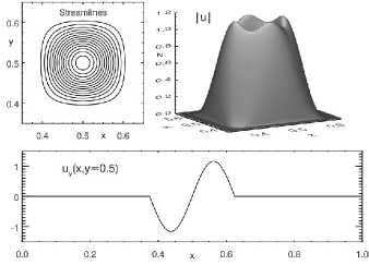
Figure 1.— Circular vortex employed as boundary velocity forcing in the presented simulations. Above: streamlines and profile of its absolute value $|u|$. Below: plot of the velocity $y$-component as a function of $x$ at $y=0.5$.

As shown in Figure 1 Equations (7)-(9) describe a counter-clockwise vortex centered in the middle of the plane $z=L$ and has circular streamlines, with a slight departure from a perfectly circular shape toward the edge of the interval I. Averaging over the surface I the velocity rms is $\langle(u^{L})^{2}\rangle_{I}=1/2$, the same value of the boundary velocity fields used in our previous works (Rappazzo et al., 2007, 2008; Rappazzo, Velli & Einaudi, 2010; Rappazzo & Velli, 2011).

In all simulations a vanishing velocity is imposed at the bottom plate $z=0$:

$$\mathbf{u}^{0}\left(x,y\right)=0.$$ (10)

At time $t=0$ we start our simulations with a uniform and homogeneous magnetic field along the axial direction $\mathbf{B}_{0}=B_{0}\,\mathbf{\hat{e}}_{z}$. The orthogonal component of the velocity and magnetic fields are zero inside our computational box $\mathbf{u_{{}_{\perp}}}=\mathbf{b_{{}_{\perp}}}=0$, while at the top and bottom planes the vortical velocity forcing is applied and kept constant in time.

We briefly summarize and specialize to the case considered in this paper the linear stage analysis described in more detail in Rappazzo et al. (2008). In general for an initial interval of time smaller than the nonlinear timescale $t<\tau_{nl}$, nonlinear terms in Equations (1)-(3) can be neglected and the equations linearized. For simplicity we will at first neglect also the diffusive terms and consider their effect later in this section. The solution during the linear stage with a generic boundary velocity forcing $\mathbf{u}^{L}$, and $\mathbf{u}^{0}=0$, (respectively at the top and bottom planes $z=L$ and $0$) is given by:

$$\mathbf{b_{{}_{\perp}}}(x,y,z,t)=\frac{t}{\tau_{A}}\,\mathbf{u}^{L},$$ (11)

$$\mathbf{u_{{}_{\perp}}}(x,y,z,t)=\frac{z}{L}\,\mathbf{u}^{L}.$$ (12)

where $\tau_{A}=L/v_{A}$ is the Alfvén crossing time along the axial direction $z$. The magnetic field grows linearly in time, while the velocity field is stationary and the order of magnitude of its rms is determined by the boundary velocity profile. Both are a mapping of the boundary velocity field $\mathbf{u}^{L}$.

For a generic forcing the solution (11)-(12) is valid only during the linear stage, while for $t>\tau_{nl}$ when the fields are big enough the nonlinear terms cannot be neglected. Nevertheless there is a singular subset of velocity forcing patterns for which the generated coronal fields (11)-(12) have a vanishing Lorentz force and the nonlinear terms vanish exactly.

This subset of patterns is characterize by having the vorticity constant along the streamlines (Rappazzo et al., 2008). In this case magnetic energy grows quadratically in time until some instability eventually sets in. Two kind of velocity patterns can be identified: a) 1D patterns with their streamlines all parallel to each other, like a shear flow, or b) a radial pattern with circular streamlines, like a circular vortex.

Since in the linear stage the coronal fields are a mapping of the boundary velocity (11)-(12), a shear flow induces a sheared magnetic field subject to tearing instabilities (Rappazzo, Velli & Einaudi, 2010), while the vortical flows considered in this paper twist the field lines into helices subject to kink instabilities. The vortex (8)-(9) is not perfectly circular as the streamlines depart from an exact round shape toward the edge (Figure 1), but as we show in § 4.1 field line tension adjusts the induced coronal orthogonal field lines in a round shape.

So far we have neglected the diffusive terms in the RMHD Equations (1)-(3). In § 4 we show that for this kind of problem the use of hyperdiffusion is crucial, otherwise the dynamics are dominated by diffusion. Overlooking this numerical fact can result in misleading conclusions (Klimchuk et al., 2009, 2010), upon which we will comment in § 4.

Here we want to understand the diffusive effects on the linear dynamics, i.e., when nonlinear terms are negligible or artificially suppressed by a low numerical resolution. We now consider the effect of standard diffusion (case $n=1$ in eqs. (1)-(2)) on the solutions (11)-(12): these are the solutions of the linearized equations obtained from (1)-(2) retaining also the diffusive terms.

In the linear regime, as the magnetic field grows in time (11), the diffusive term ($\nabla_{{}_{\!\perp}}^{2}\,\mathbf{b_{{{}_{\perp}}}}\!\propto\!\mathbf{b}_{{}_{\perp}}/\ell^{2}$) becomes increasingly bigger until diffusion balances the magnetic field growth, and the system reaches a saturated equilibrium state. Including diffusion the magnetic field evolves as

$$\mathbf{b_{{}_{\!\perp}}}(x,y,z,t)=\mathbf{u}^{L}(x,y)\frac{\tau_{R}}{\tau_{A}}\,\left[1-\exp\left(-\frac{t}{\tau_{R}}\right)\right],$$ (13)

i.e., for times smaller than the diffusive timescale $\tau_{R}$ Equation (11) is recovered with the field growing linearly in time, while for times bigger than $\tau_{R}$ the field asymptotes to its saturation value. The diffusive timescale associated with the Reynolds number $Re$ is $\tau_{R}=\ell_{c}^{2}\,Re/(2\pi)^{2}$ where $\ell_{c}$ is the length-scale of the forcing pattern, that for the pattern (7)-(9) is given by $\ell_{c}\sim\ell/4$ where $\ell$ is the orthogonal computational box length.

The total magnetic energy $E_{M}$ and ohmic dissipation rate $J$ will then be given by

$$E_{M}=\frac{1}{2}\,\int_{V}\!\mathrm{d}^{{}^{3}}x\ \mathbf{b}_{{}_{\perp}}^{2}=E_{M}^{sat}\,\left[1-\exp\left(-\frac{t}{\tau_{R}}\right)\right]^{2},$$ (14)

$$J=\frac{1}{Re}\,\int_{V}\!\mathrm{d}^{{}^{3}}x\ \mathbf{j}^{2}=J^{sat}\,\left[1-\exp\left(-\frac{t}{\tau_{R}}\right)\right]^{2}.$$ (15)

For times smaller than the diffusive timescale $\tau_{R}$ both quantities grow quadratically in time, while for $t\gtrsim 2\,\tau_{R}$ they asymptote to their saturation value $E_{M}^{sat}$ and $J^{sat}$:

$$E_{M}^{sat}=\frac{\ell_{c}^{6}c_{A}^{2}Re^{2}}{2L(2\pi)^{4}}\,\langle(u^{L})^{2}\rangle_{I},\quad J^{sat}=\frac{2\,E_{M}^{sat}}{(4\pi)^{2}\ell_{c}^{2}Re}.$$ (16)

Magnetic energy saturates to a value proportional to the square of both the Reynolds number and the Alfvén velocity, while the heating rate saturates to a value that is proportional to the Reynolds number and the square of the axial Alfvén velocity.

Even though we use grids with $\sim 512^{2}$ points in the x-y plane, the timescales associated with ordinary diffusion are small enough to affect the large-scale dynamics, inhibiting the development of instabilities and nonlinearity. The diffusive time $\tau_{{}_{n}}$ at the scale $\lambda$ associated with the dissipative terms used in Equations (1)-(2) is given by

$$\tau_{{}_{n}}\sim Re_{{}_{n}}\,\lambda^{2n}.$$ (17)

For $n=1$ the diffusive time decreases relatively slowly toward smaller scales, while for $n=4$ it decreases far more rapidly. As a result for $n=4$ we have longer diffusive timescales at large spatial scales and diffusive timescales similar to the case with $n=1$ at the resolution scale. Numerically we require the diffusion time at the resolution scale $\lambda_{min}=1/N$, where N is the number of grid points, to be of the same order of magnitude for both normal and hyper-diffusion, i.e.,

$$\frac{Re_{{}_{1}}}{N^{2}}\sim\frac{Re_{{}_{n}}}{N^{2n}}\quad\longrightarrow\quad Re_{{}_{n}}\sim Re_{{}_{1}}\,N^{2(n-1)}.$$ (18)

Then for a numerical grid with $N=512$ points that requires a Reynolds number $Re_{{}_{1}}=800$ with ordinary diffusion we can implement $Re_{{}_{4}}\sim 10^{19}$ (table 1), removing diffusive effects at the large scales and allowing, if present, the development of kink instabilities and nonlinear dynamics.

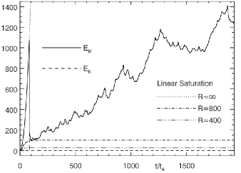
Figure 2.— Run A: Magnetic ($E_{M}$) and kinetic ($E_{K}$) energies as a function of time ($\tau_{A}=L/v_{A}$ is the axial Alfvén crossing time). The dashed curves show the time evolution of magnetic energy if the system were unperturbed [eq. (14)], or nonlinearity suppressed, e.g., by numerical diffusion (see §3). The case $R=\infty$ corresponds to the linear case with no diffusion, attained (at the large scales) with the implementation of hyperdiffusion.

4. Numerical Simulations

In this section we present the results of the numerical simulations summarized in Table 1. Simulations A and B have the same parameters, but simulation B employs a lower resolution to achieve a very long duration. In all simulations the vortical velocity pattern (7)-(9) is applied at the top plate $z=L$, and a vanishing velocity at the bottom plate $z=0$. Initially no perpendicular magnetic or velocity field is present inside the computational box $\mathbf{b}_{{}_{\!\perp}}=\mathbf{u}_{{}_{\!\perp}}=0$, and the system is threaded only by the constant and uniform field $\mathbf{B}_{0}=B_{0}\,\mathbf{\hat{e}}_{z}$. The computational box has an aspect ratio of $10$, with $\ell=1$ and $L=10$.

4.1. Run A

We present here the results of run A, a simulation performed with a numerical grid of $512\times 512\times 208$ points, and hyperdiffusion coefficient $Re_{4}=10^{19}$ with diffusivity $n=4$. The Alfvén velocity is $v_{A}=200\,\textrm{km}\,\textrm{s}^{-1}$, corresponding to a nondimensional ratio $c_{A}=v_{A}/u^{\ast}=200$. The total duration is $\sim 1,900$ axial Alfvén crossing times $\tau_{A}=L/v_{A}$.

Figures 2-3 show the temporal evolution of the total magnetic and kinetic energies

$$E_{M}=\frac{1}{2}\int\!\mathrm{d}V\,\mathbf{b}_{{}_{\!\perp}}^{2},\qquad E_{K}=\frac{1}{2}\int\!\mathrm{d}V\,\mathbf{u}_{{}_{\!\perp}}^{2},$$ (19)

the total ohmic dissipation rate

$$J=\frac{1}{Re}\int\!\mathrm{d}V\,\mathbf{j}^{2},$$ (20)

and $S$, the power injected from the boundary by the work done by convective motions on the field lines’ footpoints (see Equation (22)), along with some saturation curves for magnetic energy (14). Additionally Figure 4 shows snapshots of the magnetic field lines of the orthogonal component $\mathbf{b_{{}_{\perp}}}$ and electric current $j=j_{z}$, the leading order component in RMHD ordering (Strauss, 1976), at selected times in the mid-plane $z=5$.

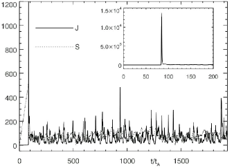
Figure 3.— Run A: Ohmic ($J$) dissipation rate and the integrated Poynting flux $S$ (the injected power) versus time. Viscous dissipation is negligible respect to the ohmic contribution. Inset shows the ohmic dissipative peak corresponding to the development of kink instability.

The circular vortical velocity field (8)-(9) applied at the top boundary ($z=10$) initially induces velocity and magnetic fields in the computational box that follow the linear behavior given by Equations (11)-(12), i.e., they are a mapping of the velocity at the boundary with the magnetic field increasing linearly in time (Figure 4, times $t=0.61\,\tau_{A}$ and $80.64\,\tau_{A}$). In the linear stage ($t\lesssim 83\,\tau_{A}$) magnetic energy is well-fitted (Figure 2) by the linear curve (14) in the limit $Re\rightarrow\infty$, i.e., in the absence of diffusion (indeed in this limit the curve can be obtained directly from the linear Equation (11)). This is because we are using hyperdiffusion that effectively gets rid of diffusion at the large scales.

Two other magnetic energy linear diffusive saturation curves are drawn for $Re=800$ and $400$, typical Reynolds numbers used in our previous simulations with standard diffusion $n=1$ and orthogonal grids with respectively $512^{2}$ and $256^{2}$ grid points (see, e.g., Rappazzo et al., 2008). Their saturation level is very low compared to the magnetic energy values when kink instability develops ($t\sim 83\,\tau_{A}$) and in the following nonlinear stage. This is because the vortex and induced magnetic field occupy only a limited volume elongated along z at the center of the x-y plane: at these scales diffusion dominates with these resolutions using standard diffusion.

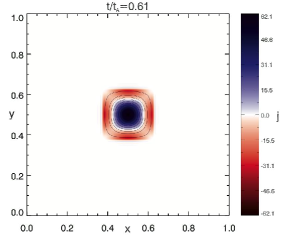
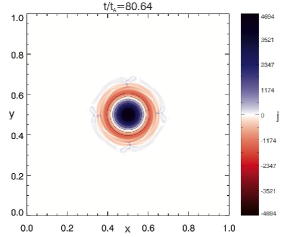
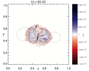
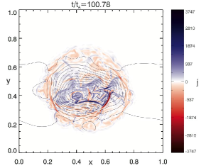
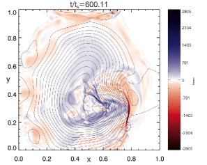
Figure 4.— Run A: Axial component of the current $j$ (in color) and field lines of the orthogonal magnetic field in the midplane ($z=5$) at selected times covering the linear and nonlinear regimes up to $t\sim 600\,\tau_{A}$. At the beginning of the linear stage ($t=0.61\,\tau_{A}$) the orthogonal magnetic field is a mapping of the boundary vortex [see linear analysis, Equation (11)]. Still in the linear stage but at later times ($t=80.64\,\tau_{A}$) the field line tension straightens out in a circular shape the vortex mapping. An internal kink mode develops ($t\sim 83.85\,\tau_{A}$) and the instability transitions the system to the nonlinear stage. In the fully nonlinear stage the field lines are still circular, but in a disordered way, exhibit a broad range of scales, including current sheets, and steadily occupy a larger fraction of the computational box.

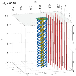
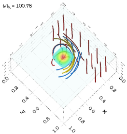
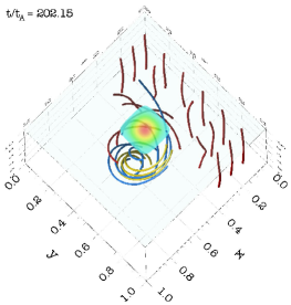
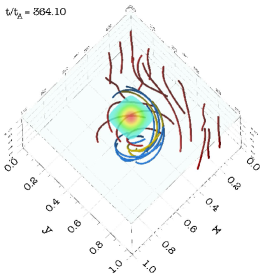
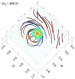
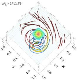
Figure 5.— Run A: Lateral and top views of magnetic field lines at selected times. In the linear stage ($t=60.57\,\tau_{A}$) the boundary vortex (shown in color in the plane $z=10$) twists into an helix the magnetic field lines in the corresponding region underneath the vortex. Those outside this region remain straight, a sample of which is shown in red. Kink instability releases magnetic energy and untwists the field lines ($t=100.78\,\tau_{A}$), that in the nonlinear stage maintain an approximately constant twist $\sim 180^{\circ}$. But with time the region where field lines are twisted increases its volume until it fills the whole computational box ($t\sim 1211.78\,\tau_{A}$). The box has been rescaled for an improved visualization, the axial length (along $z$) is ten times the length of the orthogonal cross section (along $x$-$y$). A lateral view is shown only in the first panel, at later times a top view is preferred for a better visualization, as from the side the field lines appear overlapped to each other.

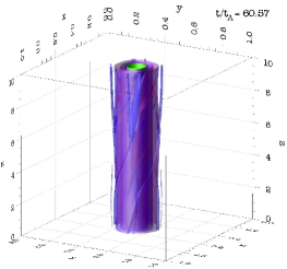
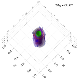
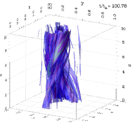
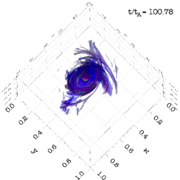
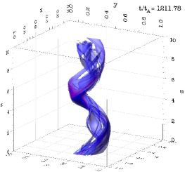
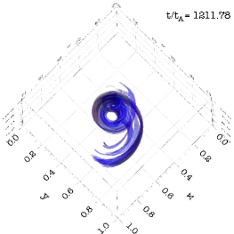
Figure 6.— Run A: Lateral (left column) and top (right column) views of isosurfaces of the squared current $j^{2}$ at selected times, respectively during the linear stage ($t\sim 60.57\,\tau_{A}$), right after kink instability ($t\sim 100.78\,\tau_{A}$), and in the fully nonlinear regime ($t\sim 1211.78\,\tau_{A}$). In each panel are shown three isosurfaces of $j^{2}$, corresponding respectively to $15\%$ (green), $5\%$ (red) and $2\%$ (blue) of the maximum of $j^{2}$ in the box at each time. As is typical of current sheets, isosurfaces corresponding to higher values of $j^{2}$ are nested inside those corresponding to lower values. Although the region where field lines are twisted increases in time (Figure 5), the current sheets’ filling factor remains small. The box has been rescaled for an improved visualization as in Figure 5.

For this reason the use of hyperdiffusion is crucial to study this problem, otherwise diffusion dominates and a balance between the injection of energy from the boundary and its numerical removal by diffusion is reached very soon, inhibiting the development of kink instability and nonlinear dynamics. This diffusive linear regime was reached in previous simulations by Klimchuk et al. (2009, 2010), where four similar vortices were applied at the boundary. Therefore their conclusion that nonlinear dynamics or instabilities (not to mention turbulence) cannot develop in such physical systems is simply a numerical issue: this can be overcome adopting hyperdiffusion as we have done here or, alternatively, implementing grids with much higher resolutions that require impractically large numerical resources.

The localized boundary vortex (shown with a colored contour in Figure 5) generates a mostly poloidal magnetic field confined to the axial volume in correspondence of the vortex, resulting in helical field lines for the total magnetic field (Figure 5, time $t=60.57\,\tau_{A}$). Outside this volume the poloidal field vanishes and only the axial field $B_{0}$ is present. Ampère’s law then guarantees that the total net current is zero. As shown in Figure 4 in the linear stage ($t=0.61\,\tau_{A}$, $80.64\,\tau_{A}$) there is a stronger up-flowing current concentrated in the middle, and a weaker ring-shaped down-flowing current distributed at the edge of the flux-tube.

This magnetic configuration is well known to be kink unstable, and is similar to the NC (Null Current) force-free model studied by Lionello et al. (1998). The main differences are that their axial field $B_{0}$ is not uniform, dropping by $\sim 50\%$ outside the flux tube, and that the field lines are line-tied to a motionless photosphere. They performed a linear stability analysis of this configuration finding that there is a critical axial loop length $L_{crit}$ beyond which the system is unstable and has a constant growth rate $\gamma\tau_{A}\sim 0.02$. They also examined other equilibria with net current finding a similar qualitative behavior, with variations for the critical length and growth rates.

Lionello et al. (1998) found that for the NC case the ratio of the axial critical length over the cross-length of the flux-tube is $L_{crit}/\ell_{c}\sim 9$. In the case considered here the ratio of the axial length ($L=10$) over the cross-length of the flux tube (the extent of the boundary vortex $\ell_{c}=1/4$, Equation (7)) is $L/\ell_{c}=40$, therefore it is fully in the unstable region. Of course at a given length (beyond the critical length) there is also a critical twist beyond which the configuration is unstable. In our simulations the system is continuously forced at the boundary, and in the linear stage the twist grows linearly in time (from Equation (11), as the twist is proportional to $b_{\perp}/B_{0}$), thus such a critical twist is certainly attained.

In our case the “equilibrium” solution is not static but is given by the linear solution (11), indicated here with $\mathbf{b}_{lin}$, with the magnetic field growing linearly in time while mapping the boundary vortex. Thus we compute the perturbed magnetic energy as

$$E_{{}_{M}}^{{}^{\star}}=\int_{V}\mathrm{d}^{{}^{3}}\!\!x\,\left|\mathbf{b}-\mathbf{b}_{lin}\right|^{2}.$$ (21)

We find that in the linear stage this quantity grows exponentially in time, obtaining for the perturbed magnetic field a growth rate $\gamma\tau_{A}\sim 0.02$, as Lionello et al. (1998) for their NC equilibrium model. This growth rate is also confirmed by the fact that kink instability sets in at $t\sim 83\,\tau_{A}$ (Figures 2 and 3) and $1/\gamma\sim 50\,\tau_{A}$. As mentioned in § 3 the forcing boundary vortex departs from an exact circular shape at its edges where its vorticity is not exactly constant along the streamlines, thus there is a small Lorenz force for the resulting magnetic field (11). This small difference in the linear field acts as a perturbation.

Additionally Lionello et al. (1998) found out that configurations with zero net current are unstable to the internal kink mode (opposed to the global kink mode for configurations with a net current), for which magnetic perturbations and the radial displacement of the plasma column are confined within the original flux tube. This is found also in our simulation as shown in Figure 4 at the onset of the nonlinear stage at $t=83.85\,\tau_{A}$, when the plasma displaces inside the flux tube toward its edge where a strong current sheet forms.

The internal kink mode releases almost 90% of the accumulated energy around time $t\sim 83.5\,\tau_{A}$ (Figure 2) in correspondence of the big ohmic dissipative peak shown in Figure 3. The released energy is $\Delta E\sim 10^{3}\times 10^{22}\,erg=10^{25}\,erg$, in the micro-flare range (the factor to convert energy into dimensional units, given our normalization choice discussed in § 3, is $10^{22}$, i.e., $1\rightarrow 10^{22}\,erg$). As a result of the kink instability magnetic reconnection occurs (Figure 4, $t=85.05\,\tau_{A}$) and the magnetic field lines get substantially unwind as shown in Figure 5 (times $t=60.57\,\tau_{A}$ and $100.78\,\tau_{A}$) with field lines twisting only $\sim 180^{\circ}$ after the instability.

In summary, during the linear stage, the transition to and the first phase of the nonlinear regime, the analysis of Lionello et al. (1998) is fully confirmed also for the photospherically driven case considered here: the system forced by a circular vortex is unstable to an internal kink mode, releases most of the stored magnetic energy and magnetic reconnection untwists the field lines. Linear calculations (Baty, 2001) show that similar dynamics are expected also for different configurations with different aspect ratios and magnetic guide field values, except for those that fall below the instability threshold.

The phenomenology described so far is also in agreement with that of three-dimensional simulations with a realistic geometry (Amari & Luciani, 2000). In particular strong nonlinearities persist right after the instability occurs ($t=85.05\,\tau_{A}$ and $100.78\,\tau_{A}$), when the system cannot be described as a constant-$\alpha$ force-free state. An inverse cascade of magnetic energy is observed, as the orthogonal magnetic field acquires longer scales and the overall volume occupied by twisted field lines increases, as shown in Figure 4 just before ($t=85.05\,\tau_{A}$) and after ($t=100.78\,\tau_{A}$) the instability. In Amari & Luciani (2000) this corresponds also to an inverse cascade of magnetic helicity, corresponding in the RMHD case to an inverse cascade of the square potential $\psi$ (see the end of this section and our discussion in § 5 for more about this quasi-invariant analogous to helicity in RMHD).

Figure 7.— Run A: Magnetic ($E_{M}$) and kinetic ($E_{K}$) time-averaged energy spectra as a function of the orthogonal wavenumber $n_{{}_{\!\perp}}$ The inset shows the kinetic energy spectrum of the boundary velocity vortex [Equations (7)-(9)] applied at the top plate $z=10$.

On the other hand, at later times the dynamics are certainly surprising when, in the fully nonlinear stage, fluctuations created by the kink instability are present in the corona. For $t>100\,\tau_{A}$ magnetic energy increases steadily, while kinetic energy remains small (Figure 2). This is in contrast to all our previous simulations with space-filling boundary motions, either distorted vortices (Rappazzo et al., 2007, 2008; Rappazzo & Velli, 2011) or shear flows (Rappazzo, Velli & Einaudi, 2010), when in the nonlinear regime a magnetically dominated statistically steady state was reached where integrated quantities would fluctuate around an average value (with velocity fluctuations smaller than magnetic fluctuations).

In our case ohmic dissipation $J$ and the integrated Poynting flux $S$ do reach a statistically steady state (Figure 3). The integrated Pointing flux

$$S=c_{A}\!\int\limits_{z=L}\!\!\mathrm{d}a\,\mathbf{b}_{{}_{\perp}}\cdot\mathbf{u}^{L},$$ (22)

is the power entering the system at the boundaries as a result of the work done by photospheric motions on the footpoints of magnetic field lines ($\mathbf{u}^{L}$ is the photospheric forcing velocity). But in contrast to our previous results, here the power does not balance on the average the dissipation rate, its average is slightly higher resulting in the magnetic energy growth shown in Figure 2.

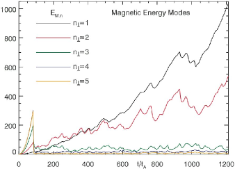
Figure 8.— Run A: Magnetic energy modes versus time. While modes with wavenumber $n_{{}_{\!\perp}}\geq 3$ fluctuate around a mean value, the first two modes increase steadily showing that an inverse cascade occurs.

In physical space the dynamics are surprising in two ways. First, after the kink instability, even though we continue to stir the field lines’ footpoints with the same vortex, no further kink instability develops. Analogously to the shear flow case (Rappazzo, Velli & Einaudi, 2010), once the system transitions to the nonlinear stage the magnetic fluctuations generated during the instability do not have a vanishing Lorentz force. In fact around $t\sim 100\,\tau_{A}$, at the end of the big dissipative event, the topology of the orthogonal component of the magnetic field is characterized by circular, but distorted, field lines (Figure 4). Naturally the Lorentz force does not vanish now and the vorticity is not constant along the streamlines. Nonlinear terms do not vanish as they do during the linear stage for $t<83\,\tau_{A}$. When they vanish magnetic energy can be stored, without getting dissipated, into an ordered flux-tube with helical field lines (Figure 5, $t=60.57\,\tau_{A}$), and matching perfectly round orthogonal magnetic field lines (Figure 4, $t=80.64\,\tau_{A}$). But now nonlinearity continuously transfers energy from large to small scales where it is dissipated. In physical space small scales are not uniformly distributed, but they are organized in field-aligned current sheets. These, once formed during the onset of the nonlinear stage, persist throughout the subsequent dynamics (as shown in Figures 4 and 6), with the energy cascade continuously feeding them. Second, the photospherical vortical motions do not give rise to an orderly helical flux-tube as in the linear stage (Figure 5, $t=60.57\,\tau_{A}$). However, magnetic field lines get twisted, but in a disordered way (Figure 5 and  4, $t\geq 100.78\,\tau_{A}$). A new phenomenon occurs: on longer timescales the magnetic field acquires longer spatial scales (Figure 4), the volume where field lines are twisted increases (Figure 5), while the current exhibits always a small filling factor occupying a small fraction of the volume (Figure 6).

To better understand these phenomena we need to investigate the energy dynamics in Fourier space. We consider the spectra in the orthogonal $x$-$y$ plane integrated along the $z$ direction. As they are isotropic in the Fourier $k_{x}$-$k_{y}$ plane we compute the integrated 1D spectra, so that for the total magnetic energy $E_{M}$ we obtain:

$$E_{M} = \frac{1}{2}\int\limits_{0}^{L}\!\mathrm{d}z\,\iint\limits_{0}^{\quad\ \ell}\!\mathrm{d}x\,\mathrm{d}y\ \mathbf{b}_{{}_{\!\perp}}^{2}$$ (23)

$$= \frac{1}{2}\int\limits_{0}^{L}\!\mathrm{d}z\ \ell^{2}\sum_{\mathbf{k}}|\hat{\mathbf{b}}|^{2}(\mathbf{k},z)=\sum_{n=1}^{N}E_{M}(n),$$

where $n$ indicates the shell in $k$-space with wavenumber $\mathbf{k}=(k,l)\in\mathbb{Z}^{2}$ included in the range $n-1<(k^{2}+l^{2})^{1/2}\leq n$, and $N$ is the maximum wavenumber admitted by the numerical grid (corresponding to the smallest resolved orthogonal scale).

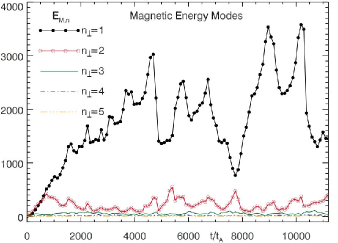
Figure 9.— RunB: Over long time-scales also the first two magnetic energy modes saturate fluctuating around a mean value. The first mode dominates, and the amplitude of its fluctuations corresponds to releases of energy of $\sim 2\times 10^{25}$ erg, in the micro-flare range.

The time averaged magnetic and kinetic energy spectra as a function of wavenumber are shown in Figure 7, the inset shows the spectrum of the boundary vortex’ kinetic energy (see Equation (7)). Photospheric motions therefore inject energy at wavenumbers between 2 and 7 (see Equation (22)), the system is magnetically dominated and the power-laws exhibited at higher wavenumbers, in the inertial range, are similar to those obtained with previous space-filling boundary forcings (Rappazzo et al., 2008; Rappazzo, Velli & Einaudi, 2010; Rappazzo & Velli, 2011), with the spectrum of magnetic energy much steeper than that of kinetic energy.

However the time-average of the low-wavenumber modes hides an interesting dynamics. Figure 8 shows the first five magnetic energy modes as a function of time. While modes with wavenumbers $n\geq 3$ after the kink instability fluctuate around a mean value, the first two modes $n=1,2$ grow steadily with mode $n=1$ becoming prevalent. This shows that an inverse cascade takes place. While the direct cascade transfers energy from the injection scale toward small scales (current sheets) where energy is dissipated, analogously the inverse cascade transfers energy toward the large scales (modes 1 and 2) where no dissipative process is at work and consequently energy accumulates. In physical space this process gives rise to the large scales that the magnetic field acquires in the orthogonal direction, shown in Figures 4 and 5, discussed previously. In the RMHD system with boundary conditions as we apply here there is no strict invariant known to follow an inverse cascade, such as magnetic helicity in 3D MHD or the square of the vector potential in 2D MHD (Biskamp, 2003; Berger, 1997; Brandenburg & Matthaeus, 2004). RMHD resembles the 2D MHD case in the sense that though the square of the vector potential is not conserved, the terms violating conservation arise only from the boundaries in the axial direction. A dynamical magnetic inverse cascade mechanism is therefore still active, impeded only by the inputs coming from photospheric motions at the boundary, and this explains the accumulation of magnetic energy at the largest transverse scales.

4.2. Run B

The simulation described in the previous section (run A) has a duration of $\sim 1200\,\tau_{A}$, but this time span leaves undetermined the behavior of the low wavenumber modes over longer time scales. Indeed these modes keep growing, as shown in Figure 8, resulting in a steady growth of total magnetic energy, shown in Figure 2. To understand the long-time dynamics of the system, we have performed another simulation, run B, with the same physical parameters of run A, but half the orthogonal resolution (Table 1), extending the duration up to $\sim 11000\,\tau_{A}$.

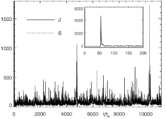
Figure 10.— RunB: Ohmic (J) dissipation rate and the integrated Poynting flux S (the injected power) versus time. Inset shows the ohmic dissipative peak corresponding to the development of kink instability.

Figure 9 shows that over longer times the energy of the system is prevalently in mode 1, i.e., the largest possible scale. But this mode does not grow indefinitely and over these much longer time-scales it reaches a statistically steady state, fluctuating around its mean value. The largest energy fluctuations shown in Figure 9 result in energy drops of $\sim 2000$, that in dimensional units correspond to a micro-flare with $\Delta E\sim 2\times 10^{25}\,erg$, releasing about twice the amount of energy released by the kink instability around $t\sim 85\,\tau_{A}$ in run A (compare with Figure 2). Notice that the kink instability does not appear in Figure 9 because the sampling time interval for the modes is too long in run B, but it is clearly shown in the r.m.s. of the energies (not shown) and in the dissipation rate (see inset in Figure 10).

Comparing Figure 9 with Figure 10, where the ohmic dissipation rate $J$ is shown as a function of time, displays another interesting result. The large and sharp energy drops shown in Figure 9 correspond to large dissipative peaks in Figure 10, e.g., at times $t\sim 4750\,\tau_{A}$ and $t\sim 10300\,\tau_{A}$, but it is also possible to have equally large but more gradual energy drops, e.g., between times $t\sim 6750\,\tau_{A}$ and $t\sim 7750\,\tau_{A}$, without a corresponding single large dissipative peak but rather a cluster of smaller peaks.

In physical space we have already seen in run A that initially the inverse cascade corresponds to a perturbed magnetic field that occupies an increasingly larger volume (Figure 4) until all the field lines in the box get twisted (Figure 5). In run B we observe that successively, once the computational box has been filled with perpendicular magnetic field, the rising amplitude of modes  1 corresponds to an increase of the magnetic field intensity, while the fluctuations in the energy mode are due to magnetic reconnection events. In fact due to the periodic boundary conditions in $x$ and $y$ the same system repeats indefinitely along these directions. When the orthogonal magnetic field reaches the boundary it starts to interact with the neighboring structures (i.e. with itself coming from the other side). The magnetic energy drops in mode 1 correspond to magnetic reconnection events that make the system oscillate between the different possible configurations with energy contained at the (large) scales of mode 1 shown in Figure 11 (there is no preferred orthogonal direction for the system at this scale).

While the periodic boundary conditions limit the interactions of large-scale twisted magnetic structures it is clearly shown that interaction with such other magnetic copies of itself is one of the ways in which the accumulated energy can be released. Further possibilities and the dynamics of these interactions will be the subject of future works.

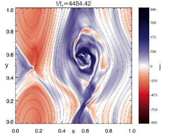
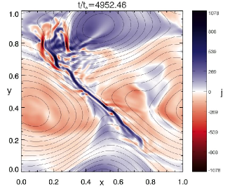
Figure 11.— Run B: Axial component of the current $j$ (in color) and field lines of the orthogonal magnetic field in the midplane ($z=5$) at times $t\sim 4484\,\tau_{A}$ and $t\sim 4952\,\tau_{A}$, i.e., just before and after the dissipative events at time $t\sim 4750\,\tau_{A}$ (Figures 9, and 10). Once the orthogonal magnetic field fills the computational box the system oscillates between the different configurations with most of the magnetic energy at the large scales, through episodes of magnetic reconnection.

5. Conclusions and Discussion

In this paper we have investigated the dynamics of a closed coronal region driven at its boundary by a localized photospheric vortex. Such small vortical motions with scales typical of photospheric convection ($\sim 1000$ km) have been recently observed in the photosphere (Brandt et al., 1988; Bonet et al., 2008, 2010), and can induce relevant dynamics in the solar corona (Velli & Liewer, 1999; Wedemeyer-Böhm et al., 2012; Panasenco, Martin, & Velli, 2013).

A “straightened out” closed region of the solar corona is modeled as an elongated Cartesian box where the top and bottom plates mimic the photosphere, and the dynamics are integrated with the Reduced MHD equations (Kadomtsev & Pogutse, 1974; Strauss, 1976), well suited for a plasma threaded by a strong axial magnetic field.

The initial condition consists simply of a uniform axial magnetic field. Its field lines are originally straight and its footpoints are line-tied at both ends in the top and bottom photospheric plates. The photospheric vortex drags the field lines’ footpoints twisting the magnetic field lines (Figure 5, $t=60.57\,\tau_{A}$). Even though the vortex that we employ is not perfectly circular (Figure 1, Equations (7)-(9)) in the linear stage the field lines’ tension straightens out in a round shape the orthogonal magnetic field lines (Figure 4, $t=0.61\,\tau_{A}$ and $t=80.64\,\tau_{A}$), in this way the Lorentz force vanishes in the planes and the system is able to accumulate energy. The small departure from a round shape (at its edge) of the boundary vortex introduces a small perturbation in the coronal field. The system is then unstable to the internal kink mode (Figure 4, $t=80.64\,\tau_{A}$), and releases about $90\%$ of the accumulated energy in a dissipative event (Figures 2 and 3). The energy released in this event is of the order of a micro-flare with $\Delta E\sim 10^{25}$ erg.

These results are in agreement with those of Lionello et al. (1998), that consider similar initial conditions, performs a refined linear analysis, but does not employ a boundary forcing, i.e., the field lines are line-tied to a motionless photosphere. Therefore the initial linear stage and the development of the kink instability are in agreement with previous works that have always employed large-scale smooth fields with no broad-band fluctuations as initial conditions, both in the case of field lines line-tied to a motionless photosphere (Baty & Heyvaerts, 1996; Velli et al., 1997; Lionello et al., 1998; Browning et al., 2008; Hood et al., 2009) and with a boundary driver (Mikíc et al., 1990; Gerrard et al., 2002).

On the other hand in the solar corona perturbations are continuously injected from the lower atmospheric layers. Numerical simulations (e.g., Rappazzo et al., 2008) confirm that especially in closed regions, where waves cannot escape toward the interplanetary medium, broad-band magnetic fluctuations of the order of a few percent of the strong axial magnetic field (not infinitesimal perturbations as classically used in instabilities studies) are naturally present.

Therefore in order to gain a first insight of the coronal dynamics when the magnetic field is already structured, i.e., there are finite magnetic fluctuations (small but not infinitesimal) with small scales and current sheets, we continue the simulation after kink instability develops. In fact right after kink instability the magnetic energy is small (Figure 2), with $b_{\perp}/B_{0}\sim 5\%$, but it is already structured with current sheets (Figure 4, $t=100.78\,\tau_{A}$) and a broad band spectrum (Figure 7).

The boundary vortex continues to twist the magnetic field lines, but in a disordered way (Figure 5, $t=202.15$ – $1211.78\,\tau_{A}$). The presence of an already structured magnetic field allows nonlinear dynamics to develop: once current sheets and small scales are present, an energy cascade continues to feed them, as shown by the energy spectra in Figure 7. Therefore current sheets do not disappear, and the continuous transfer of energy from the large to the small scales prevents the field lines to increase their twist beyond $\sim 180^{\circ}$. The twist remains approximately constant in the nonlinear stage as shown in Figure 5 ($t=202.15$ – $1211.78\,\tau_{A}$). Furthermore because the current is now concentrated in thin current sheets (Figures 4 and 6) kink instabilities do not develop.

We had already observed a similar behavior in our previous simulations that employed space-filling boundary drivers. In particular when the field lines were sheared by a 1D boundary forcing (Rappazzo, Velli & Einaudi, 2010) the coronal field was sheared only in the linear stage, but after that a multiple tearing instability developed and in the coronal field magnetic fluctuations and current sheets were formed, the continuous shearing motions at the boundary were not able to recreate a sheared coronal field and further instabilities were not observed.

But in the simulations presented in this paper a new phenomenon occurs. Although the field lines’ twist is approximately constant in the nonlinear stage, the volume where field lines are twisted increases, and the magnetic field acquires larger scales (Figures 4 and 5). Besides a direct cascade that transfers energy from the large to the small scales where it is dissipated in current sheets, an inverse cascade takes place, transferring energy from the injection scale toward larger scales, where no dissipation takes place and energy can accumulate. The analysis of the magnetic energy modes (Figures 8 and 9) shows indeed that on long time-scales most of the energy is stored at the largest possible scale (mode 1). The inverse cascade is able to store a significant amount of magnetic energy.

Although magnetic helicity is not defined in RMHD, the integral of the magnetic square potential $\psi$ is approximately conserved (see discussion in last paragraph of §4.1). The inverse cascade of magnetic energy corresponds also to an inverse cascade of the square potential, as clearly shown in Figure 4 where the field lines are the contour of $\psi$ (and $\psi\geq 0$). In future compressible simulations we expect to observe for magnetic helicity (well defined in 3D MHD) dynamics similar to those shown here for magnetic energy, i.e., an increase of magnetic helicity (injected from the boundary) and its inverse cascade, in analogy to the the inverse helicity cascade observed by Amari & Luciani (2000).

Because of the periodic boundary conditions along $x$ and $y$ the system is virtually repeated along these directions. When the field lines get twisted in the entire computational box, this twisted structure interacts with these neighboring twisted structures. This interaction is the only condition that limits the growth of magnetic energy, giving rise to impulsive magnetic reconnection events, that now is not inhibited by the circular topology of the orthogonal magnetic field lines of a single structure. These events make the system oscillate between the many possible configurations with energy in mode 1 (two of these are shown in Figure 11). The associated energy drops shown in Figure 9 are also in the micro-flare range with $\Delta E\sim 2\times 10^{25}$ erg, twice the value of the energy released initially by the kink instability.

Although in the presented simulations the generated magnetic structures interact only with similar structures repeated by the periodic boundary conditions along $x$ and $y$, we can infer that the interaction of a single twisted magnetic structure with other magnetic structures can give rise to similar release of energy. A more general investigations of the interaction between twisted magnetic structures is under way to understand under which conditions the interaction leads to energy storage and/or release, and to determine quantitatively these properties.

Previous simulations that employed a space-filling photospheric forcing (Rappazzo et al., 2008; Rappazzo, Velli & Einaudi, 2010) were not able to accumulate a significant amount of energy to be successively released in micro or larger flares. Those photospheric motions, that mimic a uniform and homogeneous convection, give instead rise to a basal background coronal heating rate in the lower range of the observational constraint ($10^{6}$ erg cm^-2 s^-1) and a million degree corona (Dahlburg et al., 2012). In the case of a space-filling boundary driver we had also observed that the inverse cascade is inhibited (see Rappazzo et al., 2008, §5.4) for typically strong DC magnetic fields. An inverse cascade is possible only for weak guide fields (see Rappazzo et al., 2008, §5.4), a condition applicable only to limited regions of the corona.

We conclude that in presence of line-tying and a strong guide field, inverse cascade can be a good mechanism to store energy, but only if the boundary motion is localized in space as the vortex used here, and not space-filling. Subsequently the interaction of this magnetic structures with others can release the accumulated energy.

In general photospheric motions will be a superposition of approximately homogenous space-filling convective motions and localized vortical and also shearing motions (e.g., see Dahlburg et al., 2009, for a localized shear case). While the space-filling motions give rise to a basal background coronal heating (e.g., Rappazzo et al., 2008), localized motions can give rise to higher impulsive releases of energy in the micro-flare range and above, contributing to coronal heating while increasing the temporal intermittency of the energy deposition and of its associated radiative emissions. In future works we will consider cases with localized motions superimposed to a homogenous space-filling convection-mimicking velocity field to determine, among other things, how stronger the localized velocity has to be respect to the background motions in order to develop dynamics similar to those presented in this paper.

As mentioned in the introduction, highly (and orderly) twisted magnetic structures, such as flux ropes, are used to initiate solar eruptions (e.g., see Török et al. (2011) for a recent application, and the reviews by Low (2001); Chen (2011) for further examples of this model). Kink-like instabilities developing in these flux-ropes give rise to an explosive dynamics leading to the formation of a CME. We have shown that kink-unstable flux ropes are not formed in the corona by boundary vortical motions, unless a very strong vortex is applied and the coronal magnetic fluctuations can then be neglected. Therefore, although flux ropes can be formed in the complex dynamics in and around a prominence region (Amari et al., 1999), given the ubiquitous presence of magnetic fluctuations in the solar corona, the development of kink-like instabilities may be strongly limited. While the dynamics of the induced CME can be a good approximation, we conclude that such models offer a poor model of the initiation process for which more realistic models are called for (Amari et al., 2011).

Generally speaking, in a realistic 3D geometry one might expect that the growth of energy in the transverse field leads to an inflation and rise of a magnetic loop due to the curvature, which we have neglected here. This effect was included by Amari et al. (1996), who showed that twisting the footpoints of a curved flux rope leads to its gradual expansion and the system rises to larger solar radii. In our simulations the twist does not increase (the overall field lines twist is limited to $180^{\circ}$), remaining roughly constant in the nonlinear stage. It is left to future work to understand under which conditions such a system, including curvature, has dynamics similar to those of Amari et al. (1996), or whether different dynamics are possible (see also Gerrard et al., 2004), and how the dynamics develop in a 3D geometry considering small or large-scales photospheric vortices.

References

- Amari & Aly (2009) Amari, T. & Aly, J. J. 2009, in IAU Symp. 257, Universal Heliophysical Processes, ed. N. Gopalswamy & D. F. Webb (Cambridge: Cambridge Univ. Press), 211
- Amari et al. (2011) Amari, T., Aly, J., Luciani, J., Mikíc, Z., Linker, J. 2011, ApJ, 742, L27
- Amari & Luciani (2000) Amari, T. & Luciani, J. F. 2000, Phys. Rev. Lett., 84, 6
- Amari et al. (1996) Amari, T., Luciani, J. F., Aly, J. J., & Tagger, M. 1996, ApJ, 466, L39
- Amari et al. (1999) Amari, T., Luciani, J. F., Mikíc, Z., & Linker, J. 1999, ApJ, 518, L57
- Baty (2001) Baty, H. 2001, A&A, 367, 321
- Baty & Heyvaerts (1996) Baty, H., & Heyvaerts, J. 1996, A&A, 308, 935
- Berger (1997) Berger, M. A. 1997, J. Geophys. Res., 102, 2637
- Bhattacharjee et al. (1998) Bhattacharjee, A., Ng, C. S., & Spangler, S. R. 1998, ApJ, 494, 409
- Biskamp (2003) Biskamp, D. 2003, Magnetohydrodynamic Turbulence (Cambridge: Cambridge Univ. Press)
- Bonet et al. (2008) Bonet, J., Márquez, I., Sánchez Almeida, J., Cabello, I. & Domingo, V. 2008, ApJ, 687, L131
- Bonet et al. (2010) Bonet, J., et al. 2010, ApJ, 723, L139
- Brandenburg & Matthaeus (2004) Brandenburg, A., & Matthaeus, W. H. 2004, Phys. Rev. E, 69, 56407
- Brandt et al. (1988) Brandt, P., Scharmer, G., Ferguson, S., Shine, R. & Tarbell, T. 1988, Nature, 335, 238
- Browning et al. (2008) Browning, P. K., Gerrard, C., Hood, A. W., Kevis, R., & Van der Linden, R. A. M. 2008, A&A, 485, 837
- Chen (2011) Chen, P. F. 2011, Living Rev. Solar Phys., 8, 1
- Dahlburg et al. (2012) Dahlburg, R. B., Einaudi, G., Rappazzo, A. F., & Velli, M. 2012, A&A, 544, L20
- Dahlburg et al. (2009) Dahlburg R. B., Liu J., Klimchuk J. A., Nigro G 2009, ApJ, 704, 1059
- Dmitruk & Gómez (1997) Dmitruk, P., & Gómez, D. O. 1997, ApJ, 484, L83
- Dmitruk & Gómez (1999) Dmitruk, P., & Gómez, D. O. 1999, ApJ, 527, L63
- Dmitruk et al. (2003) Dmitruk, P., Gómez, D. O., & Matthaeus, W. H. 2003, Phys. Plasmas, 10, 3584
- Einaudi & Velli (1999) Einaudi, G., & Velli, M. 1999, Phys. Plasmas, 6, 4146
- Einaudi et al. (1996) Einaudi, G., Velli, M., Politano, H., & Pouquet, A. 1996, ApJ, 457, L113
- Furth et al. (1963) Furth, H. P., Killeen, J., & Rosenbluth, M. N., 1963, Phys. Fluids, 6, 459
- Georgoulis et al. (1998) Georgoulis, M. K., Velli, M., & Einaudi, G. 1998, ApJ, 497, 957
- Gerrard et al. (2002) Gerrard, C. L., Arber, T. D., & Hood, A. W. 2002, A&A, 387, 687
- Gerrard et al. (2004) Gerrard, C. L., Hood, A. W., & Brown, D. S. 2004, Sol. Phys., 222, 79
- Heyvaerts & Priest (1984) Heyvaerts, J., & Priest, E. R. 1984, ApJ, 137, 63
- Hood et al. (2009) Hood A. W., Browning P. K., Van der Linden, R. A. M. 2009, A&A, 506, 913
- Kadomtsev & Pogutse (1974) Kadomtsev, B. B., & Pogutse, O. P. 1974, Sov. Phys. JETP, 38, 283
- Klimchuk et al. (2009) Klimchuk, J. A., Nigro, G., Dahlburg, R. B., & Antiochos, S. K. 2009, in American Geophysical Union, Fall Meeting 2009, abstract #SM42B-03
- Klimchuk et al. (2010) Klimchuk, J. A., Nigro, G., Dahlburg, R. B., & Antiochos, S. K. 2010, in American Astronomical Society, AAS Meeting #216, abstract #302.05, Bulletin of the American Astronomical Society, 41, 847
- Lionello et al. (1998) Lionello, R., Velli, M., Einaudi, G., & Mikíc, Z. 1998, ApJ, 494, 840
- Low (2001) Low, B. C. 2001, J. Geophys. Res., 106, 25141
- Mikíc et al. (1990) Mikíc, Z., Schnack, D. D., & Van Hoven, G. 1990, ApJ, 361, 690
- Montgomery (1982) Montgomery, D. 1982, Phys. Scr. T, 2, 83
- Panasenco, Martin, & Velli (2013) Panasenco, O., Martin, S. F., & Velli, M. 2013, ApJ, in press
- Parker (1972) Parker, E. N. 1972, ApJ, 174, 499
- Parker (1988) Parker, E. N. 1988, ApJ, 330, 474
- Parker (1994) Parker, E. N. 1994, Spontaneous Current Sheets in Magnetic Fields ( New York: Oxford Univ. Press)
- Pontin et al. (2011) Pontin, D. I., Wilmot-Smith, A. L., Hornig, G., Galsgaard, K. 2011, A&A, 525, A57
- Rappazzo & Velli (2011) Rappazzo, A. F., & Velli, M. 2011, Phys. Rev. E, 83, 065401(R)
- Rappazzo, Velli & Einaudi (2010) Rappazzo, A. F., Velli, M., & Einaudi, G. 2010, ApJ, 722, 65
- Rappazzo et al. (2007) Rappazzo, A. F., Velli, M., Einaudi, G., & Dahlburg, R. B. 2007, ApJ, 657, L47
- Rappazzo et al. (2008) Rappazzo, A. F., Velli, M., Einaudi, G., & Dahlburg, R. B. 2008, ApJ, 677, 1348
- Strauss (1976) Strauss, H. R. 1976, Phys. Fluids, 19, 134
- Taylor (1974) Taylor, J. B. 1974, Phys. Rev. Lett., 33, 1139
- Taylor (1986) Taylor, J. B. 1986, Rev. Mod. Phys., 58, 741
- Török et al. (2011) Török, T., Panasenco, O., Titov, V., Mikić, Z., Reeves, K. K., Velli, M., Linker, J., & De Toma, G. 2011, ApJ, 739, L63
- Velli & Liewer (1999) Velli, M., & Liewer, P. 1999, Space Sci. Rev., 87, 339
- Velli et al. (1997) Velli, M., Lionello, R., & Einaudi, G. 1997, Sol. Phys., 172, 257
- Wedemeyer-Böhm et al. (2012) Wedemeyer-Böhm, S., Scullion, E., Steiner, O., Rouppe van der Voort, L., de La Cruz Rodriguez, J., Fedun, V., Erdélyi, R. 2012, Nature, 486, 505
- Wilmot-Smith et al. (2011) Wilmot-Smith, A. L., Pontin, D. I., Hornig, G., Yeates, A. R. 2011, A&A, 536, A67
- Yeates et al. (2010) Yeates, A. R., Hornig, G., Wilmot-Smith, A. L. 2010, Phys. Rev. Lett., 105, 85002
- Zank & Matthaeus (1992) Zank, G. P., & Matthaeus, W. H. 1992, J. Plasma Phys., 48, 85