Multiple steady-states in nonequilibrium quantum systems with electron-phonon interactions

Abstract

The existence of more than one steady-state in a many-body quantum system driven out-of-equilibrium has been a matter of debate, both in the context of simple impurity models and in the case of inelastic tunneling channels. In this Letter, we combine a reduced density matrix formalism with the multilayer multiconfiguration time-dependent Hartree method to address this problem. This allows to obtain a converged numerical solution of the nonequilibrium dynamics. Considering a generic model for quantum transport through a quantum dot with electron-phonon interaction, we prove that a unique steady-state exists regardless of the initial electronic preparation of the quantum dot consistent with the converged numerical results. However, a bistability can be observed for different initial phonon preparations. The effects of the phonon frequency and strength of the electron-phonon couplings on the relaxation to steady-state and on the emergence of bistability is discussed.

The existence of a unique steady-state in strongly correlated quantum systems out-of-equilibrium has been a subject of great interest and controversy. For the case of the Anderson impurity model, it has been argued using the Bethe ansatz that a single steady-state solution exists Andrei2006 . However, recent calculations of the nonequilibrium current based on time-dependent density functional theory seem to indicate that at long times the system reaches a dynamical state characterized by correlation-induced current oscillations Gr2010 . Similarly, questions regarding hysteresis, bistability and the dependence of the steady-state current on the initial occupation have been raised in the context of inelastic transport through nanoscale quantum dots galperin_hysteresis_2004 ; galperin_non-linear_2008 ; Bratkovsky2007 ; Bratkovsky2009 ; Kosov2011 ; albrecht_bistability_2012 ; Komnik2013 .

Addressing the issue of a unique steady-state is a challenging task for theory, as systems exhibiting bistability involve strong electron-electron or electron-phonon correlations. Under these conditions, an exact solution is unavailable, and one has to resort to approximate methods or to numerical techniques. The former are based on either a mean-field approximation or on a perturbative scheme, where the inclusion of higher order corrections is not always clear or systematic, and thus may lead to questionable results. Numerically brute-force approaches, such as time-dependent numerical renormalization-group techniques anders_real-time_2005 ; schmitteckert_nonequilibrium_2004 ; white_density_1992 , iterative weiss_iterative_2008 ; eckel_comparative_2010 ; Segal10 or stochastic muhlbacher_real-time_2008 ; werner_diagrammatic_2009 ; schiro_real-time_2009 ; werner_weak-coupling_2010 diagrammatic methods, and wave function based approaches wang_numerically_2011 , have been very fruitful, but are limited in the range of parameters and timescales that can be studied.

In this Letter, we address the problem of a unique steady-state in a system with electron-phonon couplings. To study the nonequilibrium dynamics, we develop an approach based on a reduced density matrix (RDM) formalism, which requires as input a short-lived memory kernel cohen_memory_2011 . We show that if a steady-state exists then it must be unique, regardless of the initial electronic preparation. However, a bistability can develop for different initial phonon states. The relaxation to steady-state and the appearance of the bistability depends on the phonon frequency and the strength of the electron-phonon couplings. To illustrate this, we combine the approach with the multilayer multiconfiguration time-dependent Hartree method (ML-MCTDH) Thoss03 to numerically converge the memory kernel at short times until it decays, and infer from it the dynamics of the system at all times and the approach to steady-state.

We consider a generic model for charge transport through a quantum dot with electron-phonon interaction. The model is described by the Hamiltonian $H=H_{S}+H_{B}+V_{SB}$, where $H_{S}=\varepsilon_{d}d^{\dagger}d$ is the system (quantum dot) Hamiltonian with creation/annihilation fermionic operators $d^{\dagger}$/$d$ and energy $\varepsilon_{d}$, $H_{B}=H_{l}+H_{\mbox{ ph}}$ where $H_{l}=\sum_{k\in L,R}\varepsilon_{k}a_{k}^{\dagger}a_{k}$ represents the noninteracting leads Hamiltonian with fermionic creation/annihilation operators $a_{k}^{\dagger}$/$a_{k}$, and $H_{\mbox{p}h}=\underset{\alpha}{\sum}\omega_{\alpha}\left(b_{\alpha}^{\dagger}b_{\alpha}+\frac{1}{2}\right)$ represents the phonon bath with creation/annihilation bosonic operators $b_{\alpha}^{\dagger}$/$b_{\alpha}$ for phonon mode $\alpha$ with energy $\omega_{\alpha}$. The coupling between the system and the baths is given by $V_{SB}=V_{l}+V_{\mbox{p}h}$ where $V_{l}=\underset{k\in L,R}{\sum}\left(t_{k}da_{k}^{\dagger}+t_{k}^{*}a_{k}d^{\dagger}\right)$ is the coupling between the system and the leads with couplings strength $t_{k}$, and $V_{\mbox{p}h}=d^{\dagger}d\underset{\alpha}{\sum}M_{\alpha}\left(b_{\alpha}^{\dagger}+b_{\alpha}\right)$ is the couplings between the system and the phonon bath, where $M_{\alpha}$ is the electron-phonon couplings to mode $\alpha$.

The coupling strengths were determined by various spectral functions. The dot-leads coupling terms were determined from a spectral function of the form $\Gamma_{L,R}(\varepsilon)=2\pi\sum_{k\in L,R}|t_{k}|^{2}\delta(\varepsilon-\varepsilon_{k})$, where a tight-binding form was employed: $\Gamma_{L,R}\left(\varepsilon\right)=\frac{a^{2}}{b^{2}}\sqrt{4b^{2}-(\varepsilon-\mu_{L,R})^{2}}$ with $a=0.2\mbox{eV}$ and $b=1\mbox{eV}$. $\mu_{L,R}$ is the chemical potential of the left (L) or right (R) lead, respectively. Similarly, the electron-phonon couplings were determined from a phonon spectral function $J(\omega)=\frac{\pi}{2}\sum_{\alpha}\frac{M_{\alpha}^{2}}{\omega_{\alpha}}\delta(\omega-\omega_{\alpha})$, where $J\left(\omega\right)=\frac{\pi}{2}\eta\omega e^{-\frac{\omega}{\omega_{c}}}$ is taken to be of Ohmic form. The dimensionless Kondo parameter, $\eta=\frac{\lambda}{2\omega_{c}}$, determines the overall strength of the electron-phonon couplings where $\lambda=\sum\frac{M_{\alpha}^{2}}{2\omega_{\alpha}}=\frac{1}{\pi}\int\frac{d\omega}{\omega}J(\omega)$ is the reorganization energy (or polaron shift) and $\omega_{c}$ is the characteristic phonon bath frequency.

Following the derivation outlined in Ref. cohen_memory_2011, for the Anderson impurity model, the equation of motion for the RDM, $\sigma(t)=Tr_{B}\{\rho(t)\}$, is given by

$$i\hbar\frac{\partial}{\partial t}\sigma\left(t\right)=\mathcal{L}_{S}\sigma\left(t\right)+\vartheta\left(t\right)-\frac{i}{\hbar}\int_{0}^{t}d\tau\kappa\left(\tau\right)\sigma\left(t-\tau\right)$$ (1)

where $\mathcal{L}_{S}=[H_{S},\cdots]$ is the system’s Liouvillian, $Tr_{B}\{\cdots\}$ is a trace over the baths degrees of freedom (leads and phonon baths) and $\rho(t)$ is the full density matrix. In the above,

$$\vartheta\left(t\right)=Tr_{B}\left\{\mathcal{L}_{V}e^{-\frac{i}{\hbar}Q\mathcal{L}t}Q\rho\left(0\right)\right\}$$ (2)

depends on the choice of initial conditions and vanishes for an uncorrelated initial state (which is the case discussed below), i.e. when $\rho(0)=\sigma(0)\otimes\rho_{B}(0)$, where $\sigma(0)$ and $\rho_{B}(0)$ are the system and baths initial density matrices, respectively, and $\mathcal{L}_{v}=[V_{SB},\cdots]$. The memory kernel, which describes the non-Markovian dependency of the time propagation of the system, is given by

$$\kappa\left(t\right)=Tr_{B}\left\{\mathcal{L}_{V}e^{-\frac{i}{\hbar}Q\mathcal{L}t}Q\mathcal{L}\rho_{B}\right\}$$ (3)

where $Q=1-P$, $P=\rho_{B}(0)Tr_{B}\{\cdots\}$ and $\mathcal{L}=[H,\cdots]$.

To obtain $\sigma(t)$, one requires as input the super-matrix of the memory kernel, which can be expressed in terms of a Volterra equation of the second type, removing the complexity of the projected dynamics of Eq. (3):

$$\kappa\left(t\right)=i\hbar\dot{\Phi}\left(t\right)-\Phi\left(t\right)\mathcal{L}_{S}+\frac{i}{\hbar}\int_{0}^{t}d\tau\Phi\left(t-\tau\right)\kappa\left(\tau\right)$$ (4)

with

$$\Phi\left(t\right)=Tr_{B}\left\{\mathcal{L}_{V}e^{-\frac{i}{\hbar}\mathcal{L}t}\rho_{B}\right\}.$$ (5)

Evaluating the super-matrix $\Phi(t)$ requires a tedious calculation similar to that carried out in Ref. cohen_memory_2011, . The diagonal matrix elements $\Phi_{ii,mm}(t)$ are given by $\frac{2}{\hbar}\Im\left\{\varphi_{mm}(t)\right\}$, where

$$\varphi_{mn}(t)=Tr_{B}\left\{\rho_{B}\left\langle n\right|\underset{k}{\sum}t_{k}d(t)a_{k}^{\dagger}(t)\left|m\right\rangle\right\}.$$ (6)

The indices $i$, $j$, $m$, and $n$ can take the values $1$ or $0$, corresponding to an occupied or an unoccupied dot, respectively. The off-diagonal elements of $\Phi_{ij,nm}(t)$ are given by $\delta_{j1}\delta_{i0}\psi_{mn}(t)+\delta_{j0}\delta_{i1}\psi_{nm}^{*}(t)$, where

$$\begin{split}\psi_{mn}(t)&=Tr_{B}\left\{\rho_{B}\left\langle n\right|\underset{k}{\sum}t_{k}a_{k}^{\dagger}(t)\right.\\ &-\left.d^{\dagger}(t)\underset{\alpha}{\sum}M_{\alpha}\left(b_{\alpha}^{\dagger}(t)+b_{\alpha}(t)\right)\left|m\right\rangle\right\}.\end{split}$$ (7)

Since both the operator $d(t)a_{k}^{\dagger}(t)$ appearing in the equation for $\varphi_{mn}(t)$ and the full Hamiltonian conserve the total particle number, $\varphi_{mn}(t)$ is nonzero only for $m=n$, in which case it has a simple physical interpretation as the time derivative of the dot population. $\varphi_{mm}(t)$ can be expressed in terms of the sum of the left and right currents $e\varphi_{mm}(t)=I^{L}_{m}(t)+I^{R}_{m}(t)$, where:

$$I^{L,R}_{m}(t)=-\frac{2e}{\hbar}\Im\underset{k\in L,R}{\sum}t_{k}\langle m|d(t)a_{k}^{\dagger}(t)|m\rangle,$$ (8)

and $e$ is the electron charge. In addition, one can show that $\psi_{mn}(t)$ is nonzero only for $m\neq n$. As a result, the populations and coherences of $\sigma(t)$ are decoupled cohen_memory_2011 , and if one is interested in the behavior of the populations alone, only $\varphi_{mm}(t)$ is required. The resulting equations of motion for the diagonal elements of $\sigma(t)$ are given by:

$$\frac{\partial}{\partial t}\sigma_{ii}\left(t\right)=-\frac{1}{\hbar^{2}}\underset{m}{\sum}\int_{0}^{t}d\tau\kappa_{ii,mm}\left(\tau\right)\sigma_{mm}\left(t-\tau\right).$$ (9)

If $\sigma(t)$ has a steady-state solution as $t\rightarrow\infty$, then $\frac{\partial}{\partial t}\sigma_{ii}\left(t\right)=0$, and $\underset{m}{\sum}\int_{0}^{\infty}d\tau\kappa_{ii,mm}\left(\tau\right)\sigma_{mm}\left(t-\tau\right)=0$ can be replaced by a linear set of equations given by:

$$\underset{m}{\sum}\mathcal{K}_{im}\sigma_{m}=0,$$ (10)

where $\mathcal{K}_{im}=\frac{1}{\hbar^{2}}\int_{0}^{\infty}d\tau\kappa_{ii,mm}\left(\tau\right)$ and $\sigma_{m}\equiv\sigma_{mm}(t\rightarrow\infty)$. The matrix $\mathcal{K}$ in Eq. (10) has two eigenvalues. The first is $\lambda_{0}=0$ corresponding to $\sigma_{00}=\frac{\mathcal{K}_{00}}{\mathcal{K}_{00}+\mathcal{K}_{11}}$ and $\sigma_{11}=1-\sigma_{00}=\frac{\mathcal{K}_{11}}{\mathcal{K}_{00}+\mathcal{K}_{11}}$. For a physical steady-state solution, both $\mathcal{K}_{00}$ and $\mathcal{K}_{11}$ must share the same sign. Otherwise, the diagonal elements of $\sigma$ cannot both be positive. The other eigenvalue is $\lambda_{1}=\mathcal{K}_{00}+\mathcal{K}_{11}$ corresponding to $\sigma_{00}=-\sigma_{11}=1$, which can never represent a physical solution. Furthermore, since the steady-state depends only on the value of $\mathcal{K}_{00}$ and $\mathcal{K}_{11}$ and since both are independent of the initial dot population, the steady-state is independent of the initial preparation of the dot occupation and therefore, is unique.

The steady-state solution is unique with respect to the electronic initial preparation. This is a strong statement by itself, but it does not rule out bistability for different initial phonon preparations. To address this question, we combined the formalism described above for the RDM with the ML-MCTDH approach in second quantized representation (SQR) Wang2009 ; wang_numerically_2011 . The ML-MCTDH-SQR provides a tool to compute the currents in Eq.(8) numerically exactly. The kernel $\kappa(t)$ is then obtained by numerically solving Eq. (4). In comparison, for most model parameters studied in this work, it is practically impossible to obtain converged values for the RDM directly from the ML-MCTDH-SQR, since the time to reach a steady-state solution is significantly longer than the maximum simulation time reachable by the ML-MCTDH-SQR. However, since the memory kernel decays on much shorter timescales compared to the RDM itself cohen_memory_2011 , it is rather straightforward to calculate it using the ML-MCTDH-SQR and then solve Eq. (9) for the RDM.

To characterize the population dynamics, we start with a factorized initial condition of the form $\rho\left(0\right)=\sigma\left(0\right)\otimes\rho_{\mbox{ph}}\left(0\right)\otimes\rho_{\mbox{leads}}(0)$, where $\sigma\left(0\right)$ determines whether the electronic level is initially occupied/unoccupied, $\rho_{\mbox{ph}}\left(0\right)=\exp\left[-\beta\left\{\underset{\alpha}{\sum}\omega_{\alpha}\left(b_{\alpha}^{\dagger}b_{\alpha}+\frac{1}{2}\right)+\underset{\alpha}{\sum}\delta_{\alpha}\left(b_{\alpha}^{\dagger}+b_{\alpha}\right)\right\}\right]$ represents the initial density matrix of the phonon bath. Hereby two values of the parameters $\delta_{\alpha}$ are considered: $\delta_{\alpha}=0$ (corresponding to a phonon initial state equilibrated with an unoccupied dot) and $\delta_{\alpha}=\sqrt{2\omega_{\alpha}\lambda}$ (corresponding to phonons equilibrated to an occupied dot). $\rho_{\mbox{leads}}(0)=\exp\left[-\beta\left(\underset{k\in L}{\sum}\left(\varepsilon_{k}-\mu_{L}\right)a_{k}^{\dagger}a_{k}+\underset{k\in R}{\sum}\left(\varepsilon_{k}-\mu_{R}\right)a_{k}^{\dagger}a_{k}\right)\right]$ determines the initial density matrix for the leads. In the above $\beta=\frac{1}{k_{B}T}$ is the inverse temperature. In all results shown below we take $T=0$ and $\mu_{L}=-\mu_{R}=0.05$eV.

In Fig. 1 we plot the time evolution of $\sigma_{11}(t)$ (lower panels) and the corresponding nonzero elements of the memory kernel (upper panels), for two different initial vibrational preparations. We show the time evolution of $\sigma_{11}(t)$ for different values of the cutoff time $t_{c}$ at which we assume that the memory kernel has essentially decayed to zero, such that it can be safely truncated. For $\delta_{\alpha}=0$, it is safe to truncate the memory kernel at $t_{c}>30\mbox{fs}$ while $\delta_{\alpha}=\sqrt{2\omega_{\alpha}\lambda}$ requires a larger cutoff time of $t_{c}>80\mbox{fs}$. Comparing the time it takes for the memory kernel to decay (upper panels of Fig. 1) with the time taken by the RDM to reach steady-state (corresponding lower panels of Fig. 1), it is clear that the latter is slower by nearly an order of magnitude and in some cases even more. Since the calculation of the memory kernel using the ML-MCTDH-SQR is by far the most time consuming portion of the calculation, the combination with the RDM formalism provides a significant saving, and more importantly extends the ML-MCTDH-SQR approach to regimes inaccessible by direct application.

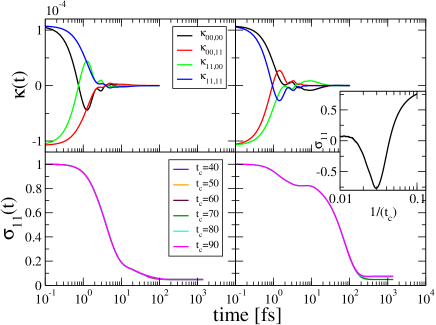
Figure 1: The occupation of the quantum dot $\sigma_{11}(t)$ (lower panels) for different cutoff times and the nonzero elements of the memory kernel (upper panels) for $\delta_{\alpha}=0$ (left panels) and $\delta_{\alpha}=\sqrt{2\omega_{\alpha}\lambda}$ (right panels). The inset shows the steady-state value of $\sigma_{11}$ for the case of $\delta_{\alpha}=\sqrt{2\omega_{\alpha}\lambda}$ as a function of $1/t_{c}$. The model parameters used are: $\varepsilon_{d}=0.5$eV, $\omega_{c}=500\mbox{cm}^{-1}$, and $\lambda=3000\mbox{cm}^{-1}$.

The inset of Fig. 1 shows the steady-state value of $\sigma_{11}$ as a function of $1/t_{c}$ for $\delta_{\alpha}=\sqrt{2\omega_{\alpha}\lambda}$. For large values of $1/t_{c}$ (short cutoff times) we find that the formalism may lead to unphysical situations in which $\sigma_{11}$ becomes negative. Of course, this is expected, since only when the memory kernel has decayed to zero does the cutoff approximation provide a physical meaningful solution. As $1/t_{c}$ decreases $\sigma_{11}$ converges and approaches a plateau value. In the present case of parameters, the steady-state value of $\sigma_{11}$ computed for the two initial vibrational states roughly coincides. However, the dynamics and timescales to relax to the steady-state are clearly sensitive to the initial vibrational preparation.

In Fig. 2 we plot $\sigma_{11}(t)$ for four different values of $\omega_{c}$ and compare the time dependence for four different initial conditions, corresponding to an initial empty ($n_{d}=0$) or occupied ($n_{d}=1$) dot and to $\delta_{\alpha}=0$ or $\delta_{\alpha}=\sqrt{2\omega_{\alpha}\lambda}$. For a given $\delta_{\alpha}$, we find that $\sigma_{11}(t)$ has a unique steady-state solution regardless of the initial dot occupation. This numerically converged result is consistent with the analytical proof given above. In contrast, for two different initial vibrational states, a clear bistability is observed and the RDM decays to a different steady-state solution depending on the value of $\delta_{\alpha}$. We note in passing that a similar phenomenon is known to occur at equilibrium, for example at $T=0$ in the spin-boson model Wang2008 ; Weissbook .

The appearance of a bistability is consistent with predictions based on a mean field treatment, which is accurate in the adiabatic limit where $\omega_{c}\rightarrow 0$ galperin_non-linear_2008 . For all four frequencies studied, the adiabatic effective potentials Kosov2011a shows two distinct minima (upper panel of Fig. 2), corresponding to two possible stable configurations adiabatic . The height of the barrier between the two minima is independent of the phonon frequency, however, as clearly evident in the figure, the width of the barrier increases as $\omega_{c}$ decreases. This implies that the tunneling time between the two configurations also increases as $\omega_{c}$ decreases, and thus, the bistability (given by the difference between $\sigma_{11}$ at steady-state for $\delta_{\alpha}=0$ and $\delta_{\alpha}\neq 0$) would increase with decreasing $\omega_{c}$, as indeed is the case.

The transient dynamics and the approach to steady state depends sensitively on the preparation, in particular, whether the initial state is close to equilibrium ($\{n_{d}=0,\delta_{\alpha}=0\}$ and $\{n_{d}=1,\delta=\sqrt{2\omega_{\alpha}\lambda}\}$) or far from equilibrium ($\{n_{d}=0,\delta_{alpha}=\sqrt{2\omega_{\alpha}\lambda}\}$ and $\{n_{d}=1$, $\delta_{\alpha}=0\}$). For small $\omega_{c}$ we observe a rapid decay to steady state when the initial preparation is close to equilibrium, while for the nonequilibrium preparation, the population of the dot $\sigma_{11}(t)$ decays to steady state on a time scale $\hbar\Gamma^{-1}$, where $\Gamma$ denotes the maximum of leads spectral function. As $\omega_{c}$ increases, the dynamics becomes more complex. In particular, a longer time scale in the relaxation of $\sigma_{11}(t)$ developes, consistent with the appearance of a slow tunneling channel between the two configurations. However, the existence of this channel does not lead to a unique steady state solution for the populations at a finite value of $\omega_{c}$, away from the adiabatic limit.

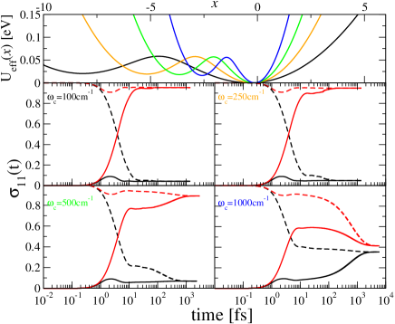
Figure 2: Plots of the occupation of the quantum dot $\sigma_{11}(t)$ for different $\omega_{c}$. The solid black, dashed black, solid red, and dashed red curves correspond to $\{n_{d}=0,\delta_{\alpha}=0\}$, $\{n_{d}=1,\delta_{\alpha}=0\}$, $\{n_{d}=0,\delta_{\alpha}=\sqrt{2\omega_{\alpha}\lambda}\}$, and $\{n_{d}=1,\delta_{\alpha}=\sqrt{2\omega_{\alpha}\lambda}\}$, respectively. Upper panel shows the adiabatic effective potentials for the different values of $\omega_{c}$. The model parameters used are: $\varepsilon_{d}=0.5$eV, and $\lambda=4000\mbox{cm}^{-1}$.

In Fig. 3 we show $\sigma_{11}(t)$ for different values of the reorganization energy (polaron shift) $\lambda$ and the dot energy $\varepsilon_{d}$. As before, we compare the time dependence of $\sigma_{11}(t)$ for four different initial conditions. In the upper panel we show the corresponding adiabatic effective potentials Kosov2011a for the four values of $\lambda$. For small values of $\lambda$, the bistability clearly disappears (left panels of Fig 3). This is consistent with the adiabatic effective potentials showing a single minimum for $\lambda\leq 3000\mbox{cm}^{-1}$ (in fact, a crude estimate based on a mean-field approach suggests that below $\lambda=3150\mbox{cm}^{-1}$ the bistability vanishes for the current parameters). Comparing the relaxation time for $\lambda=2000\mbox{cm}^{-1}$ and $\lambda=3000\mbox{cm}^{-1}$, we find that the latter is slower, particularly for the case of $\delta_{\alpha}=\sqrt{2\omega_{\alpha}\lambda}$.

When $\lambda$ is further increased to $4000\mbox{cm}^{-1}$ (corresponding to a nearly symmetric case where the polaron shift equals $\varepsilon_{d}$) the relaxation time stretches even more and the system decays to a different steady-state depending on the value of $\delta_{\alpha}$, again consistent with the appearance of two stable configurations in the corresponding adiabatic effective potential (upper panel of Fig. 3). While the RDM shows a distinct bistability, it is interesting to note that this is not the case for the current through the quantum dot (not shown), which has a unique steady state for the symmetric case ($\lambda\approx\varepsilon_{d}$).

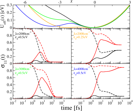
Figure 3: Similar to Fig. 2 but for different values of $\lambda$ and $\varepsilon_{d}$, for $\omega_{c}=500\mbox{cm}^{-1}$. Upper panel shows the adiabatic effective potentials for the different values of $\lambda$.

In the upper right panel of Fig. 3 we show results for the case where $\lambda=2000\mbox{cm}^{-1}$ and $\varepsilon_{d}=0.25$eV. The effective adiabatic potential for this case clearly shows two distinct minima, however, the barrier is lower than $\lambda=4000\mbox{cm}^{-1}$ and $\varepsilon_{d}=0.5$eV. Comparing the two right panels of Fig. 3, we find that as $\lambda$ and $\varepsilon_{d}$ are decreased simultaneously, the bistability decreases and the timescale to relax to steady-state also decreases, consistent with the adiabatic tunneling picture discussed above.

In this work, we have combined a RDM formalism with the ML-MCTDH-SQR approach to study the nonequilibrium dynamics of a many-body quantum system with electron-phonon couplings. For a generic model, which is widely used to describe phonon-coupled electron transport in quantum dots and single-molecule junctions, we showed that the system may exhibit pronounced bistability. The analysis reveals that the bistability increases for decreasing phonon frequency and depends sensitively on the electron-phonon coupling. This was rationalized in terms of the timescales of phonon tunneling between the two adiabatic configurations, the phonon relaxation time, and the electron relaxation. Based on the RDM formalism, we proved that the bistability is associated with different initial phonon preparations and not with a different initial dot occupations. The present results are expected to be of relevance for the interpretation of recent experiments on charge transport in molecular junction, which showed hysteretic behavior Li03 ; Loertscher06 ; Liljeroth07 , and may facilitate further experimental studies in the field of nanoelectronics.

The authors would like to thank Michael Galperin, Abe Nitzan, and Avi Schiller for useful discussion. EYW is grateful to The Center for Nanoscience and Nanotechnology at Tel Aviv University for a doctoral fellowship. HW acknowledges the support from the National Science Foundation CHE-1012479. GC is grateful Yad Hanadiv Rothschild Foundation for the award of a Rothschild Fellowship. MT and ER are grateful to the Institute of Advanced Studies at the Hebrew University for the warm hospitality. This work was supported by the FP7 Marie Curie IOF project HJSC, by the DFG (SFB 953 and cluster of excellence EAM), and used resources of the National Energy Research Scientific Computing Center, which is supported by the Office of Science of the U.S. Department of Energy under Contract No. DE-AC02-05CH11231.

References

- (1) B. Doyon and N. Andrei, Phys. Rev. B 73, 245326 (2006)
- (2) S. Kurth, G. Stefanucci, E. Khosravi, C. Verdozzi, and E. K. U. Gross, Phys. Rev. Lett. 104, 236801 (2010)
- (3) M. Galperin, M. A. Ratner, and A. Nitzan, Nano Lett. 5, 125 (2004)
- (4) M. Galperin, A. Nitzan, and M. A. Ratner, J. of Phys.: Condens. Matter 20, 374107 (2008)
- (5) A. S. Alexandrov and A. M. Bratkovsky, J. Phys. Condens. Matter 19, 255203 (2007)
- (6) A. S. Alexandrov and A. M. Bratkovsky, Phys. Rev. B 80, 115321 (2009)
- (7) A. A. Dzhioev and D. S. Kosov, J. Chem. Phys. 135, 174111 (2011)
- (8) K. F. Albrecht, H. Wang, L. Mühlbacher, M. Thoss, and A. Komnik, Phys. Rev. B 86, 081412 (2012)
- (9) A. O. Gogolin and A. Komnik, “Multistable transport regimes and conformational changes in molecular quantum dots,” arXiv 0207513
- (10) F. B. Anders and A. Schiller, Phys. Rev. Lett. 95, 196801 (2005)
- (11) P. Schmitteckert, Phys. Rev. B 70, 121302 (2004)
- (12) S. R. White, Phys. Rev. Lett. 69, 2863 (1992)
- (13) S. Weiss, J. Eckel, M. Thorwart, and R. Egger, Phys. Rev. B 77, 195316 (2008)
- (14) J. Eckel, F. Heidrich-Meisner, S. G. Jakobs, M. Thorwart, M. Pletyukhov, and R. Egger, New J. Phys. 12, 043042 (2010)
- (15) D. Segal, A. J. Millis, and D. R. Reichman, Phys. Rev. B 82, 205323 (2010)
- (16) L. Mühlbacher and E. Rabani, Phys. Rev. Lett. 100, 176403 (2008)
- (17) P. Werner, T. Oka, and A. J. Millis, Phys. Rev. B 79, 035320 (2009)
- (18) M. Schiró and M. Fabrizio, Phys. Rev. B 79, 153302 (2009)
- (19) P. Werner, T. Oka, M. Eckstein, and A. J. Millis, Phys. Rev. B 81, 035108 (2010)
- (20) H. Wang, I. Pshenichnyuk, R. Härtle, and M. Thoss, J. Chem. Phys. 135, 244506 (2011)
- (21) G. Cohen and E. Rabani, Phys. Rev. B 84, 075150 (2011)
- (22) H. Wang and M. Thoss, J. Chem. Phys. 119, 1289 (2003)
- (23) H. Wang and M. Thoss, J. Chem. Phys. 131, 024114 (2009)
- (24) H. Wang and M. Thoss, New J. Phys. 10, 115005 (2008)
- (25) U. Weiss, Quantum Dissipative Systems (World Scientific, Singapore, 1999)
- (26) A. A. Dzhioev and D. S. Kosov, J. Chem. Phys. 135, 074701 (2011)
- (27) To obtain the adiabatic potential the multiphonon problem was represented by a single mode with potential . The adiabatic effective potential is then given by the integral over the mean force where is the dot energy at position , and , where is the lesser Green function for a fixed phonon coordinate obtained by solving the nonequilibrium Green function on the Keldysh contour (see Ref. [26]).
- (28) C. Li, D. Zhang, X. Liu, S. Han, T. Tang, C. Zhou, W. Fan, J. Koehne, J. Han, M. Meyyappan, A. M. Rawlett, D. W. Price, and J. M. Tour, Appl. Phys. Lett. 82, 645 (2003)
- (29) E. Lörtscher, J. Ciszek, J. Tour, and H. Riel, Small 2, 973 (2006)
- (30) P. Liljeroth, J. Repp, and G. Meyer, Science 317, 1203 (2007)