Higgs Bosons in Warped Space, from the Bulk to the Brane

Abstract

In the context of warped extra-dimensional models with all fields propagating in the bulk, we address the phenomenology of a bulk scalar Higgs boson, and calculate its production cross section at the LHC as well as its tree-level effects on mediating flavor changing neutral currents. We perform the calculations based on two different approaches. First, we compute our predictions analytically by considering all the degrees of freedom emerging from the dimensional reduction (the infinite tower of Kaluza Klein modes (KK)). In the second approach, we perform our calculations numerically by considering only the effects caused by the first few KK modes, present in the 4-dimensional effective theory. In the case of a Higgs leaking far from the brane, both approaches give the same predictions as the effects of the heavier KK modes decouple. However, as the Higgs boson is pushed towards the TeV brane, the two approaches seem to be equivalent only when one includes heavier and heavier degrees of freedom (which do not seem to decouple). To reconcile these results it is necessary to introduce a type of higher derivative operator which essentially encodes the effects of integrating out the heavy KK modes and dresses the brane Higgs so that it looks just like a bulk Higgs.

I Introduction

Warped extra dimensional models have become very popular because they are able to address simultaneously two intriguing issues within the Standard Model (SM): the hierarchy problem and the mass/flavor problem. They were originally introduced to treat the first issue RS in a setup where the SM fields were all localized at one boundary of the extra dimension. Later it was realized that by allowing fields to propagate into the bulk, different geographical localization of fields along the extra dimension could help explain the observed masses and flavor mixing among quarks and leptons bulkSM ; fermionsbulk . Flavor bounds and precision electroweak tests put pressure on the mass scale of new physics in these models bounds , but extending the gauge groups and/or matter content (e.g. extensions ) or by slightly modifying the spacetime warping of the metric (e.g softmodels ), it is possible to keep the new physics scale at the TeV level at the reach of the Large Hadron Collider (LHC).

Electroweak symmetry breaking can still happen via a standard Higgs mechanism in these scenarios (although it can also be implemented as as Pseudo-Nambu-Goldstone boson (PNGB) pgbhiggs or described within the effective theory formalism Giudice:2007fh ; Low:2009di ). As the LHC announced the discovery of a light Higgs-like particle of a mass around 125 GeV LHCHiggs , it becomes crucial to have a detailed prediction of the properties of the physical Higgs particle in these models. The Higgs boson itself must be located near the TeV boundary of the extra dimension in order to solve the hierarchy problem, and so typically it is assumed to be exactly localized on that boundary (brane Higgs scenario). Nevertheless, it is possible that it leaks out into the bulk (bulk Higgs scenario), and in doing so indirectly alleviate some of the bounds plaguing these models AAZ .

The calculation of the production cross section of the brane Higgs in these scenarios has been addressed before Lillie:2005pt ; Falkowski:2007hz ; Djouadi:2007fm ; Bouchart:2009vq ; Cacciapaglia:2009ky ; ATZ2 ; Neubert but we will pay close attention to the more recent works of Bouchart:2009vq ; ATZ2 ; Neubert . The towers of fermion Kaluza-Klein (KK) modes will affect significantly the SM prediction and in ATZ2 it was found that the Higgs boson production rate can receive important corrections, either enhancing or suppressing the Standard Model prediction. The suppression or enhancement depends on the model parameters considered, in particular on the phases appearing in the different Yukawa-type operators present in the 5D action. Previously, the analysis of Bouchart:2009vq , in which only the first few modes were considered, gave no contribution to the rate from the towers of KK fermions. Finally, the analysis of Neubert seems to indicate that with just a few KK modes a substantial effect is obtained, but of opposite sign as the one predicted from summing the infinite tower ATZ2 .

In this work we consider the effects of allowing the Higgs boson to propagate in the bulk, with its profile more or less localized towards the IR brane depending on the value of the mass parameter $\beta$, related to the bulk mass of the 5D Higgs field.

To keep matters as simple as possible we will set up a model containing a single family of up-type 5D fermions along with a bulk Higgs scalar. Generalization to a more realistic scenario is straight forward but we prefer to stay as transparent as possible due to the many subtleties involved in the calculation.

We first compute the contribution of the complete tower of KK fermions to the Higgs production cross section as well as to the tree-level shift happening between the light fermion mass and its Yukawa coupling (leading to flavor violating couplings when considering three fermion families). These calculations, as outlined in ATZ1 ; ATZ2 , are analytically straightforward and allow us to obtain simple and compact results. We then repeat the same analysis numerically from the point of view of an effective theory in which only the first few KK fermions contribute. We show that for a bulk Higgs with a thickness of the order of inverse TeV scale, the results obtained are the same as the results obtained by summing the complete KK tower (i.e. heavier modes decouple). Moreover, these results are consistent with the predictions obtained in ATZ1 ; ATZ2 for the specific case of a brane localized Higgs. The two aproaches outlined seem to give different predictions as the bulk Higgs is continuously pushed towards the brane. It turns out that in order to maintain the consistency of both approaches we need to include in the analysis the effects of a special type of higher order operators. After these effects are included, we will come back and address in the discussion section the differences among the existing calculations in the literature and stress the importance of including the mentioned higher order operators in the analysis.

Our paper is organized as follows. In Sec. II we summarize the simple 5D warped space model used in the calculation. In Sec. III we present analytical results for the Higgs flavor-changing effects (III.1) and production (III.2), using the full tower of KK fermions. We use numerical methods to calculate the effects of including just a few KK modes in Sec. IV, both for flavor-changing neutral currents effects (IV.1) and Higgs boson production (IV.2). We include the effect of the higher order operator in Sec. V and discuss the misalignment between the Higgs boson profile and its vacuum expectation value (VEV) in Sec. VI. We discuss the significance of our results, compare them to previous analyses and conclude in Sec. VII. We leave some of the details for the Appendices A and B.

II The Model

We consider the simplest 5D warped extension of the SM, in which we keep the SM local gauge groups and just extend the space-time by one warped extra dimension.

The spacetime metric is the usual Randall-Sundrum form RS :

$$ds^{2}=\frac{R^{2}}{z^{2}}\!\Big{(}\eta_{\mu\nu}dx^{\mu}dx^{\nu}-dz^{2}\Big{)},$$ (1)

with the UV (IR) branes localized at $z=R$ ($z=R^{\prime}$). We denote the $SU(2)_{L}$ doublets by ${\cal Q}^{i}(x,z)$ and the $SU(2)_{L}$ singlets by ${\cal U}^{j}(x,z)$ where $i,j$ are flavor indices and $x$ represents the 4D spacetime coordinates while $z$ represents the extra dimension coordinate. The fermions are expected to propagate in the bulk bulkSM ; fermionsbulk .

The up-sector fermion action that we consider is therefore

$$S_{fermion}=\int d^{4}xdz\sqrt{g}\left[{i\over 2}\left(\bar{{\cal Q}_{i}}\Gamma^{A}{\cal D}_{A}{\cal Q}_{i}-{\cal D}_{A}\bar{{\cal Q}_{i}}\Gamma^{A}{\cal Q}_{i}\right)+{c_{q_{i}}\over R}\bar{{\cal Q}_{i}}{\cal Q}_{i}+\right.$$

$$\left.{i\over 2}\left(\bar{{\cal U}_{j}}\Gamma^{A}{\cal D}_{A}U_{j}-{\cal D}_{A}\bar{{\cal U}_{j}}\Gamma^{A}{\cal U}_{j}\right)+{c_{u_{j}}\over R}\bar{{\cal U}_{j}}{\cal U}_{j}\ +\ \left(Y^{*}_{ij}\ \bar{{\cal Q}_{i}}{H}{\cal U}_{j}+h.c.\right)\right],\ \ \$$ (2)

with ${\cal D}_{A}$ being the covariant derivative, and we have added a Yukawa interaction with a Higgs field $H$ which in principle can be either brane or bulk localized. From the 5D fermion mass terms one defines dimensionless parameters $c_{u_{i}}$, $c_{q_{i}}$ which are a priori quantities of ${\cal O}(1)$. The coefficients $Y^{*}_{ij}$ have inverse energy units ($1/\sqrt{\Lambda}$) since Yukawa couplings in 5D are higher dimensional operators.

After separating 5D fields into left and right chiralities we impose a mixed ansatz for separation of variables

$$q_{L}(x,z) = q_{L}^{0}(z)q_{L}^{0}(x)+\ Q_{L}^{1}(z)\Psi_{L}^{1}(x)+...\,,$$ (3)

$${q}_{R}(x,z) = q^{0}_{R}(z){u}^{0}_{R}(x)+\ Q_{R}^{1}(z)\Psi_{R}^{1}(x)+...\,,$$ (4)

$$u_{L}(x,z) = u^{0}_{L}(z)q_{L}^{0}(x)+\ U_{L}^{1}(z)\Psi_{L}^{1}(x)+...\,,$$ (5)

$${u}_{R}(x,z) = u^{0}_{R}(z){u}_{R}^{0}(x)+\ U_{R}^{1}(z)\Psi^{1}_{R}(x)+...\,,$$ (6)

where $q^{0}_{L}(x)$ and $u^{0}_{L}(x)$ are the SM fermions and $\Psi^{n}_{L,R}(x)$ are the heavier KK modes. In order to obtain a chiral spectrum, we choose boundary conditions for the fermion wavefunctions

$$q_{L}(++),\quad q_{R}(--),\quad u_{L}(--),\quad u_{R}(++),$$ (7)

so that before electroweak symmetry breaking only $q^{0}_{L}$ and $u^{0}_{R}$ will be massless (zero modes) with wavefunctions:

$$q_{L}^{0}(z) = f(c_{q})\frac{{R^{\prime}}^{-\frac{1}{2}+c_{q}}}{R^{2}}z^{2-c_{q}},$$ (8)

$$u_{R}^{0}(z) = f(-c_{u})\frac{{R^{\prime}}^{-\frac{1}{2}-c_{u}}}{R^{2}}z^{2+c_{u}},$$ (9)

where we have defined $f(c)\equiv\sqrt{\frac{1-2c}{1-\epsilon^{1-2c}}}$ and the hierarchically small parameter $\epsilon=R/R^{\prime}\approx 10^{-15}$. Thus, if we choose $c_{q}(-c_{u})>1/2$, the zero mode wavefunctions are localized towards the UV brane; if $c_{q}(-c_{u})<1/2$, they are localized towards the IR brane.

In order to implement minimally the Higgs sector out of a 5D scalar we use the following action gaugephobic

$${\cal S}_{\text{Higgs}}=\int dzd^{4}x\left(\frac{R}{z}\right)^{3}\left[Tr|{\cal{D}}_{M}H|^{2}-\frac{\mu^{2}}{z^{2}}Tr|H|^{2}\right]-V_{UV}(H)\delta(z-R)-V_{IR}(H)\delta(z-R^{\prime}),$$ (10)

where $\mu$ is the 5D mass for the Higgs boson. The boundary potentials $V_{UV}(H)$ and $V_{IR}(H)$ yield boundary conditions that can accommodate electroweak symmetry breaking, so that one obtains a Higgs VEV with a non-trivial profile along the extra-dimension. Around that VEV, one should then add perturbations and obtain the spectrum of physical modes, i.e. a SM-like Higgs boson and a tower of KK Higgs fields. The expansion should look like

$$H(x,z)=v_{\beta}(z)+h_{\beta}(z)h(x)+....,$$ (11)

and we can choose the boundary conditions such that the profile of the Higgs VEV $v_{\beta}(z)$ takes the simple form

$$v_{\beta}(z)=V(\beta)\ z^{2+\beta},$$ (12)

where $\beta=\sqrt{4+\mu^{2}}$ and

$$V(\beta)=\sqrt{\frac{2(1+\beta)}{R^{3}(1-(R^{\prime}/R)^{2+2\beta})}}\frac{v_{4}}{(R^{\prime})^{1+\beta}},$$ (13)

where $v_{4}$ is the SM Higgs boson VEV. One should note that the wave function $h_{\beta}(z)$ of the light physical Higgs (lightest KK Higgs field) will have the form

$$h_{\beta}(z)=\frac{v_{\beta}(z)}{v_{4}}\left(1+{\cal O}\left(\frac{m_{h}^{2}{z}^{2}}{1+\beta}\right)\right),$$ (14)

so that for a light enough Higgs boson mass both profiles $h_{\beta}(z)$ and $v_{\beta}(z)$ are aligned (i.e. proportional to each other).

The previous bulk Higgs sector is capable of reproducing the brane Higgs limit, since the wavefunction of the light Higgs (and its VEV) both depend exponentially on the parameter $\beta$. As this parameter is increased, the wavefunctions are pushed more and more towards the IR brane mimicking a perfectly localized Higgs sector. Indeed, the wave function of the Higgs can act as a brane localizer since

$$\lim_{\beta\to\infty}h^{2}(z)=\lim_{\beta\to\infty}v^{2}(z)=\delta(z-R^{\prime}),$$ (15)

where the Dirac delta function is defined as the limit of a sequence of functions with increasing value of $\beta$. One can easily prove that for any wavefunction $f(z)$ (or a product of wavefunctions) we have

$$\lim_{\beta\to\infty}\int_{R}^{{R^{\prime}}^{+}}h^{2}(z)f(z)\,dz=f(R^{\prime}).\$$ (16)

There is however an issue about localizing the whole Higgs sector towards the brane since we just showed that only quadratic Higgs operators will “become” brane localizers. When a 5D action operator contains more than two (or less than two) Higgs fields, the (successful) localization of such operators is not guaranteed. In fact in order to ensure that the 5D bulk Higgs scenario correctly tends smoothly to a fully localized Higgs sector, one should implement a prescription enforcing a precise $\beta$ dependence on the coefficients of all operators containing Higgs fields. More precisely, the coefficient $Y^{N}(\beta)$ of an operator containing $N$ Higgs fields (before electroweak symmetry breaking) should behave as

$$Y^{N}(\beta)=Y^{N}_{1}\times\beta^{\frac{2-N}{2}},$$ (17)

where $Y^{N}_{1}=Y^{N}(1)$. This is the only way to ensure that we can have

$$\lim_{\beta\to\infty}\int_{R}^{{R^{\prime}}^{+}}Y^{N}(\beta)\ h^{N}(z)f(z)\,dz=\lim_{\beta\to\infty}\int_{R}^{{R^{\prime}}^{+}}Y_{1}^{N}\ \beta^{\frac{2-N}{2}}h^{N}(z)f(z)\,dz=Y^{N}_{1}\ f(R^{\prime}),\$$ (18)

or in other words

$$\lim_{\beta\to\infty}Y^{N}(\beta)\ h^{N}(z)=Y^{N}_{1}\ \delta(z-R^{\prime}).$$ (19)

In particular for 5D Yukawa type couplings this prescription implies that the 5D Yukawa coupling will have to carry a $\sqrt{\beta}$ dependence in order to ensure that the brane limit Yukawa coupling is non-vanishing Agashe:2006iy (see also ATZ1 ). But it also means that any other 5D action operator containing a single Higgs field would need to carry the same $\sqrt{\beta}$ dependence. On the other hand, 5D action operators containing 3 Higgs fields (like the operator $H^{2}HQU$) would have a diverging limit for $\beta$ large unless its action coefficient $Y^{3}(\beta)$ is itself suppressed by $1/\sqrt{\beta}$.

The previous prescription makes it technically possible to define a localized Higgs sector from a 5D bulk Higgs field, but it certainly seems quite contrived to appropriately fix all operator coefficients such that they all can give non-zero and finite contributions when the Higgs is localized. A brane localized Higgs sector could seem “un-generic” or “un-natural” if it is to be seen as a limiting case of a bulk Higgs. More details about the complete prescription for operators containing Higgs fields are presented in Appendix B.

III Higgs phenomenology: all KK fermions

For completeness and consistency, we present first a result previously obtained in ATZ1 , namely the computation of the shift between the light SM fermion mass term and its Yukawa coupling with the Higgs field (leading to Higgs mediated FCNC when more than one fermion family is considered). We then calculate the coupling between the physical Higgs and two gluons for the 5D bulk Higgs case.

We can follow two routes to obtain our predictions. The computation of the flavor violating couplings of the Higgs scalar with fermions will be obtained in an approach based on considering first electroweak symmetry breaking and then solving the 5D equations of motion for the fermions (i.e. the effect of the Higgs VEV is directly taken into account in the equations of motion and during the dimensional reduction procedure). The alternative (and equivalent) approach would be to consider first the dimensional reduction (i.e. obtain the 4D effective theory in the gauge basis), and then consider the electroweak symmetry breaking in the presence of the infinite tower of KK fermions. After performing the diagonalization of the infinite fermion mass matrix (as well as canonical normalization of the fermion kinetic terms) we should recover the same results. We use the first approach in the first subsection, and the second approach in the computation of the Higgs coupling to gluons and also in the following sections where we will truncate the infinite mass matrix in order to consider only the effect of the first few KK modes.

III.1 Higgs Flavor violating couplings

After imposing electroweak symmetry breaking in the Higgs sector, the four profiles $q_{L,R}(z)$ and $u_{L,R}(z)$ introduced in eqs. (3) to (6) must obey the coupled equations coming from the equations of motion:

$$-m_{u}\ q_{L}-q^{\prime}_{R}+{c_{q}+2\over z}q_{R}+\left({R\over z}\right)v_{\beta}(z)Y_{u}\ u_{R}=0,$$ (20)

$$-m^{*}_{u}\ q_{R}+q^{\prime}_{L}+{c_{q}-2\over z}q_{L}+\left({R\over z}\right)v_{\beta}(z)Y_{u}\ u_{L}=0,$$ (21)

$$-m_{u}\ u_{L}-u^{\prime}_{R}+{c_{u}+2\over z}u_{R}+\left({R\over z}\right)v_{\beta}(z)Y^{*}_{u}\ q_{R}=0,$$ (22)

$$-m^{*}_{u}\ u_{R}+u^{\prime}_{L}+{c_{u}-2\over z}u_{L}+\left({R\over z}\right)v_{\beta}(z)Y^{*}_{u}\ q_{L}=0,$$ (23)

where the ^′ denotes derivative with respect to the extra coordinate $z$ and $Y_{u}$ is 5D Yukawa coupling.

It is simple to deduce from these equations an exact expression for the mass eigenvalue $m_{u}$ in terms of the fermion profiles ATZ1

$$m_{u}=R^{4}\int^{R^{\prime}}_{R}\!\!dz\left(\frac{m_{u}}{z^{4}}(|u_{L}|^{2}+|q_{R}|^{2})+{Rv_{\beta}(z)\over z^{5}}(Y_{u}u_{R}q^{*}_{L}\!-\!Y^{*}_{u}q_{R}u^{*}_{L})\right),\ \$$ (24)

and compare it to the expression of the fermion Yukawa coupling, i.e

$$y^{u}_{4}=R^{5}\int^{R^{\prime}}_{R}dz{h_{\beta}(z)\over z^{5}}(Y_{u}u_{R}q_{L}^{*}+Y^{*}_{d}q_{R}u_{L}^{*}),$$ (25)

where $h_{\beta}(z)$ is the profile of the physical Higgs field.

With these two expressions we compute the shift (or misalignment) between the fermion mass $m_{u}$ and the Yukawa coupling $y^{u}_{4}$ as

$$\Delta^{u}=m_{u}-v_{4}\ y^{u}_{4},$$ (26)

which becomes simply

$$\Delta^{u} = R^{4}\int^{R^{\prime}}_{R}\!\!dz\left(\frac{m_{u}}{z^{4}}(|u_{L}|^{2}+|q_{R}|^{2})-2Y^{*}_{u}{Rv_{\beta}(z)\over z^{5}}q_{R}u_{L}^{*}\right).\$$ (27)

In order to proceed further, a perturbative approach is used, such that we assume that $(\tilde{Y}_{u}v_{4}R^{\prime})\ll 1$ where $v_{4}$ is the SM Higgs VEV. Knowing the analytical form of the VEV profile $v_{\beta}(z)$ and using the $(\tilde{Y}_{u}v_{4}R^{\prime})$ small parameter it is possible to solve perturbatively the system of coupled equations (20) to (23) to any order in $(\tilde{Y}_{u}v_{4}R^{\prime})$ (see ATZ1 for details). The result for the shift in the top quark Yukawa coupling is

$$\frac{\Delta^{t}_{1}}{m{v_{4}}} =\frac{2m_{t}^{2}}{{v_{4}}}R^{\prime 2}\frac{2+c_{u}-c_{q}+\beta}{(1-2c_{q})(1+2c_{u})}\left[\frac{1}{6+c_{u}-c_{q}+3\beta}-\frac{1}{5+2c_{u}+2\beta}\right.$$ (28)

$$\left.\hskip 28.45274pt-\ \frac{1}{5-2c_{q}+2\beta}+\frac{1}{4+c_{u}-c_{q}+\beta}\right],$$

where we have only included the contribution from the third term in eq. (47), as the other terms are subdominant for light quarks, although not necesarily for the top quark. For clarity we omit their analytical expression here, but the complete analytical result can be found in ATZ1 and in the Appendix A of this work. The shift in the Yukawa coupling has some dependence on the Higgs localization parameter $\beta$ and it is shown in Figure 1 as the “infinite sum” result, as the procedure we followed is equivalent to diagonalizing the infinite fermion mass matrix in the gauge eigenbasis.

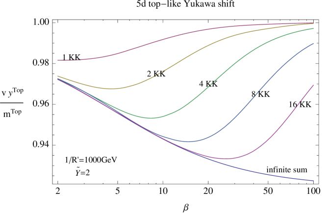
Figure 1: (color online). The shift in the top quark Yukawa coupling as a function of the bulk Higgs localization parameter $\beta$. Each line represents an effective theory containing the given amount of KK fermions. The lower line (blue) represents the contribution from the infinite tower of KK modes. Apart from the direct phenomenological impact of this result, this term also affects the $hgg$ coupling, as discussed in the text. The dimensionless 5D Yukawa couplings are fixed at $\tilde{Y}=2$ and the KK scale is set at $\displaystyle\frac{1}{R^{\prime}}=1000$ GeV (the overall effect scales as $\tilde{Y}^{2}v^{2}R^{\prime 2}$).

III.2 Higgs production

In this section we follow the approach of working with the infinite fermion KK modes with wavefunctions in the gauge basis. This is not the physical basis after electroweak symmetry breaking since Yukawa couplings will introduce off-diagonal terms in the infinite fermion mass matrix, which should be properly diagonalized in order to obtain the physical basis.

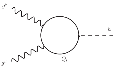
Figure 2: Loop diagram showing the contribution of the quark $Q_{i}$ to the Higgs-gluon-gluon coupling. In the SM, the dominant contribution is through the top quark due to its large Yukawa coupling with the Higgs boson. In RS the heavier KK fermions contribute to the coupling with potentially large effects, either suppressing or enhancing the SM coupling, depending on the phases present in the different Yukawa-type operators present in the 5D action, and on the localization of the Higgs (see text for details).

Since the Higgs field is not charged under QCD the main contribution to its coupling to gluons comes from a top quark loop, as shown in Figure 2; if the model contains many heavy quarks the resulting cross section for the process is $gg\to h$ is higgs

$$\sigma^{SM}_{gg\rightarrow h}={\alpha_{s}m_{h}^{2}\over 576\pi}\left|\sum_{Q}{y_{Q}\over m_{Q}}A_{1/2}(\tau_{Q})\right|^{2}\delta({\hat{s}}-m_{h}^{2}),$$ (29)

with $\tau_{Q}\equiv m^{2}_{h}/4m_{Q}^{2}$, $\hat{s}$ being the $gg$ invariant mass squared and $Q$ representing the physical fermions with physical Yukawa couplings $Y_{Q}$ and masses $m_{Q}$. The form factor is given by

$$A_{1/2}(\tau)={3\over 2}[\tau+(\tau-1)f(\tau)]\tau^{-2},$$ (30)

with

$$f(\tau)=\begin{cases}[\text{arcsin}\sqrt{\tau}]^{2}\qquad\;\qquad\;\qquad{\tau\leq 0}\\ -{1\over 4}\left[\text{ln}\left({1+\sqrt{1-\tau^{-1}}\over 1-\sqrt{1-\tau^{-1}}}\right)-i\pi\right]^{2}{\tau>1}.\end{cases}$$ (31)

Here we want to figure out the contribution to the $hgg$ coupling coming from 5D quark doublets and a singlets, i.e. containing the SM quarks (which includes doublets and singlets $(q_{L},u_{R})$), along with the associated towers of vector-like KK fermions, $(Q_{L},U_{R})$. The relevant quantity to calculate is

$$c_{hgg}=\sum_{Q}{y_{Q}\over m_{Q}}A_{1/2}(\tau_{Q}),$$ (32)

where $y_{Q}$ is the physical Yukawa coupling of the physical Dirac fermion $Q$ and $m_{Q}$ is its mass. As stated before, it will prove useful to work in the gauge basis, and so we represent the Yukawa couplings between the KK fermions $Q_{L}(x)$ and $U_{R}(x)$ in the gauge basis as $Y_{Q_{L}U_{R}}$. Its values will be obtained by performing the overlap integral of the Higgs profile and the corresponding bulk fermionic wave functions, i.e.

$$Y_{Q_{L}U_{R}}^{u}=Y^{u}\int_{R}^{R^{\prime}}dz\left({R\over z}\right)^{5}\frac{v_{\beta}(z)}{v_{4}}Q_{L}^{u(i)}(z)U_{R}^{(k)}(z),$$ (33)

where we have assumed that the nontrivial Higgs VEV and the physical Higgs profile are perfectly aligned. The Yukawa couplings between different chirality KK fermions and also between zero modes and heavy KK fermions are obtained and written in a similar way so that we can write the infinite dimensional fermion mass matrix as

$$\begin{pmatrix}\bar{q}_{L}^{u(0)}&\bar{Q}_{L}^{u(i)}&\bar{U}_{L}^{(j)}\end{pmatrix}\begin{pmatrix}Y^{u}_{{q}_{L}u_{R}}\ v_{4}&0&Y^{u}_{{q}_{L}U_{R}}\ v_{4}\\ Y^{u}_{{Q}_{L}u_{R}}\ v_{4}&M_{Q}&Y^{u}_{{Q}_{L}U_{R}}\ v_{4}\\ 0&Y^{u*}_{{U}_{L}Q_{R}}\ v_{4}&M_{U}\end{pmatrix}\begin{pmatrix}u_{R}^{(0)}\\ Q_{R}^{u(k)}\\ U_{R}^{(l)}\end{pmatrix},$$ (34)

where $M_{Q}=\text{diag}(M_{Q_{1}},M_{Q_{2}},...)$ and $M_{U}=\text{diag}(M_{U_{1}},M_{U_{2}},...)$ are the KK mass matrices for the corresponding fermion fields in the gauge basis, and we have suppressed fermion family indices to simplify notation. From eqs. (30) and (31), we notice that in eq. (29) the form factors, $A_{1/2}\approx 0$ for light fermions, and $A_{1/2}\approx 1$ for the much heavier KK modes and the top quark. Therefore, separating the contribution of the light fermions from the heavy ones we write

$$c_{hgg}=\sum_{\rm light}{y_{Q}\over m_{Q}}A_{1/2}(\tau_{Q})+\sum_{\rm heavy}{Y_{Q}\over M_{Q}},$$ (35)

where in the first (second) term the sum is only over light (heavy) fermion generations. Noting that

$$\sum_{\rm heavy}{Y_{Q}\over M_{Q}}+\sum_{\rm light}{y_{Q}\over m_{Q}}=\text{Tr}(\mathbf{YM}^{-1}),$$ (36)

where $\mathbf{M}$ is the fermion mass matrix given in (34), while $\mathbf{Y}$ is the Yukawa matrix, we have

$$c_{hgg}=\text{Tr}(\mathbf{YM}^{-1})+\sum_{\rm light}{y_{Q}\over m_{Q}}(A_{1/2}(\tau_{Q})-1).$$ (37)

We also note that $Y={\partial M\over\partial{v_{4}}}$ and since the trace is invariant under unitary transformations, we can compute it in the gauge basis (so we can use the fermion mass matrix in that basis). Up to first order in ${v_{4}}$ one finds

$$\text{Tr}(\mathbf{YM}^{-1})={\partial\text{ln Det}(\mathbf{M})\over\partial{v_{4}}}\approx{1\over{v_{4}}}-{v_{4}}\sum_{i,j}{2\over M_{Q_{i}}M_{U_{j}}}\left(Y^{u}_{{Q_{L}}_{i}{U_{R}}_{j}}Y^{u*}_{{U_{L}}_{j}{Q_{R}}_{i}}-{Y^{u}_{q_{L}{U_{R}}_{j}}Y^{u*}_{{U_{L}}_{j}{Q_{R}}_{i}}Y^{u}_{{Q_{L}}_{i}u_{R}}\over Y^{u}_{q_{L}u_{R}}}\right).\ \ \ \ \ \$$ (38)

Noting that the SM masses and Yukawa couplings are also modified (shifted) as ATZ1

$${y_{Q}\over m_{Q}}\big{|}_{\text{light}}\approx{1\over{v_{4}}}\left(1+2{{v_{4}}^{2}\over Y^{u}_{q_{L}u_{R}}}\sum_{i,j}{Y^{u}_{q_{L}{U_{R}}_{j}}Y^{u*}_{{U_{L}}_{j}{Q_{R}}_{i}}Y^{u}_{{Q_{L}}_{i}u_{R}}\over M_{Q_{i}}M_{U_{j}}}\right),$$ (39)

we can write the total $hgg$ coupling as

$$c_{hgg}=-2{v_{4}}\sum_{i,j}{Y^{u}_{{Q_{L}}_{i}{U_{R}}_{j}}Y^{u*}_{{U_{L}}_{j}{Q_{R}}_{i}}\over M_{Q_{i}}M_{U_{j}}}+{y_{Q}\over m_{Q}}\big{|}_{\text{light}}A_{1/2}(\tau_{Q_{\rm light}}).$$ (40)

where we have used equations (37), (38) and (39). As we mentioned before, the form factor is negligible for the light fermion generations. Therefore neglecting the last term above, and using (33) we have

$$c_{hgg}=-2{v_{4}}Y^{u}Y^{u*}R\sum_{i,j}\int dzdz^{\prime}\left({R\over z}\right)^{5}\left({R\over z^{\prime}}\right)^{5}{Q^{(i)}_{L}(z)Q^{(i)}_{R}(z^{\prime})\over M_{Q_{i}}}{U^{(j)}_{R}(z)U^{(j)}_{L}(z^{\prime})\over M_{U_{j}}}h_{\beta}(z)h(z^{\prime}),\ \ \ \$$ (41)

where the 5D bulk physical Higgs profiles can be normalized as gaugephobic

$$h_{\beta}(z)=\sqrt{{2(1+\beta)\over R^{3}(1-\epsilon^{2+2\beta})}}R^{\prime}\left({z\over R^{\prime}}\right)^{2+\beta},$$ (42)

with $\epsilon\equiv R/R^{\prime}\sim 10^{-15}$ being the warp factor. The sums in eq. (40) are given by ATZ2

$$\sum_{i=1}^{\infty}{Q^{(i)}_{L}(z)Q^{(i)}_{R}(z^{\prime})\over M_{Q_{i}}}=-{z^{\prime 2+c_{q}}z^{2-c_{q}}\over R^{4}}\left[\theta(z^{\prime}-z)-{(z^{\prime}/R)^{1-2c_{q}}-1\over\epsilon^{2c_{q}-1}-1}\right],$$ (43)

and

$$\sum_{j=1}^{\infty}{U^{(j)}_{R}(z)U^{(j)}_{L}(z^{\prime})\over M_{U_{j}}}={z^{2+c_{u}}z^{\prime 2-c_{u}}\over R^{4}}\left[\theta(z^{\prime}-z)-{(z^{\prime}/R)^{1+2c_{u}}-1\over\epsilon^{-2c_{u}-1}-1}\right].$$ (44)

Substitution of these sums and of the Higgs profile in Eq. (41) and assuming $\beta\geq 2$ will finally give the total Higgs coupling for the light fermions which is given in Appendix I. If we assume that $c_{q}>1/2$ and $c_{u}<-1/2$, which is the case for light fermions (up-like fermion), the expression for $c_{hgg}$ can be simplified as

$$c^{Up}_{hgg}\approx{v_{4}}Y^{u}Y^{u*}R^{\prime 2}{2(1+\beta)\over(2+\beta+c_{q}-c_{u})}{1\over 4+2\beta}.$$ (45)

In the case of the top quark, we have to add the contribution due to the last term in Eq. (40), since $A_{1/2}(\tau_{top})\sim 1$. Following the notation in ATZ1 , we write the additional contribution as

$${y_{Q}\over m_{Q}}\big{|}_{\text{light}}A_{1/2}(\tau_{Q_{light}})+{\Delta_{2}^{top}\over m_{t}{v_{4}}},$$ (46)

where the first term is given by eq. (39) multiplied by the form factor, $A_{1/2}$ and last term, is the result of kinetic term corrections due to the shift in Yukawa couplings, which are also not negligible for the heavy fermions. The shift is given by

$$\Delta_{2}^{top} = R^{4}\int^{R^{\prime}}_{R}\!\!dz\left(\frac{m_{t}}{z^{4}}(|u_{L}|^{2}+|q_{R}|^{2})\right).\$$ (47)

For a complete discussion on this, we refer the reader to ATZ1 .

So finally for IR localized fermions with $c_{q}<1/2$ and $c_{u}>-1/2$ (top-like) we have

$$c^{Top}_{hgg} \approx {y_{Q}\over m_{Q}}\big{|}_{\text{light}}A_{1/2}(\tau_{Q_{light}})+{\Delta_{2}^{top}\over m_{t}{v_{4}}}$$ (48)

$$\ -{v_{4}}Y^{u}Y^{u*}R^{\prime 2}\left[-{1\over 4+2\beta}+{1\over 2\beta+5-2c_{q}}+{1\over 2\beta+5+2c_{u}}-{1\over\beta+4-c_{q}+c_{u}}\right].$$

Following our ansatz for localizing the Higgs sector, and in order to compare with previous brane Higgs results, we need to replace the $5D$ Yukawa couplings with the dimensionless and $\beta$-independent couplings

$$\tilde{Y}={\sqrt{2(1+\beta)}\over(2-c_{q}+c_{u}+\beta)}Y^{5D}.$$ (49)

The results obtained in this section, of the contribution of a 5D top-like quark and a 5D up-like quark to the $hgg$ coupling are shown in both panels of Figure 3 as the “infinite sum” result.

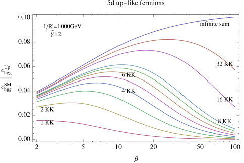
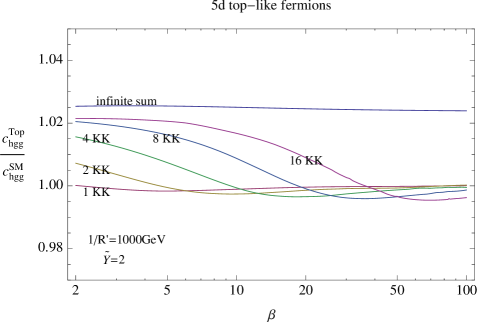
Figure 3: Contribution to $c_{hgg}/c_{hgg}^{SM}$ coming from the KK partners of the “up” quark (left panel) and from the full top quark sector (right panel) as a function of the bulk Higgs localization parameter $\beta$. Each line represents the numerical result obtained in an effective theory containing the amount of KK fermions indicated. The upper line (blue) represents the contribution of the infinite tower of KK modes (computed in the text analytically). The dimensionless 5D Yukawas are fixed at $\tilde{Y}=2$ and the KK scale is set at $\displaystyle\frac{1}{R^{\prime}}=1000$ GeV (the overall effect scales as $\tilde{Y}^{2}v^{2}R^{\prime 2}$).

IV Higgs phenomenology: individual KK modes

In this section we take a different approach and compute the effects on Higgs phenomenology (FCNC and production cross section) due to only the first few KK fermions in the model. That is, we consider a 4-dimensional effective theory which contains the SM matter content, augmented by a few levels of KK fields. This procedure is better fitted within the framework we work in (low cut-off effective theories), the drawback being that it is not possible to obtain general analytical predictions in a close form. Our strategy will be to assign some generic values to the parameters of the model and perform the computations numerically. In particular we will fix the bulk mass parameters of the 5D fermions $Q$ and $U$ to be $c_{u}=-0.6$ and $c_{q}=0.6$ (for an up-type quark) and $c_{u}=0$ and $c_{q}=0.4$ (for a top quark). The value of the dimensionless 5D Yukawa coupling will be taken to be $\tilde{Y}^{5D}_{1}=2$.

IV.1 Higgs Flavor violating couplings

In order to evaluate the shift in the Yukawa coupling of the SM fermion (the zero mode) due to the presence of a finite number of KK fermions, we can simply use Eq. (39), with the understanding that now the sum is finite, and so we shall sum up to the maximum number of KK modes chosen. We are interested in computing the top quark Yukawa shift as it is the most interesting for direct phenomenology, and also because it will also enter in the calculation of the $hgg$ coupling. We perform the sum numerically and stop the summation at different maximum numbers of KK fermions. The results are shown in Figure 1 in which we focus on the variation of the Yukawa coupling shift with respect to the bulk Higgs localization parameter $\beta$ and we compare these to the results obtained in the previous section for the infinite KK degrees of freedom. The main observation is that for small $\beta$, the finite sums are in good agreement with the infinite sum result. On the other hand for large values of $\beta$ the Yukawa shift obtained from the finite sums becomes more and more irrelevant and is clearly at odds with the infinite sum prediction.

IV.2 Higgs production

To evaluate the contribution to the $hgg$ coupling coming from the individual KK fermion modes we proceed as in the previous subsection. We now use Eq. (41), and sum up to the maximum number of KK modes desired. We perform the sum numerically and show the results in Figure 3. Again we are interested in the variation of the couplings with $\beta$ and compare them to the result for the $c_{hgg}$ obtained by calculating the infinite sum, as shown in the previous section.

The two panels of the figure show the contribution to the $hgg$ coupling coming from a 5D up-like quark (left panel) and the contribution coming from a 5D top-like quark (right panel) for $\beta$ values up to 100. We can see how the sums over different maximum number of KK modes converge to the infinite sum limit as we vary $\beta$. The approximation obtained by considering just a few KK modes is much better for low values of $\beta$. For example, from the left panel of Figure 3, for $\beta=2\to 5$, 8 KK modes saturate some 90% of the infinite sum, while for $\beta=20$, 8 KK modes saturate some 60% of the infinite sum. For $\beta=100$ (corresponding to a Higgs highly localized towards the brane), 8 KK modes represent only some 10% of the total KK contribution. This dependence on $\beta$ is in agreement with the results found in Bouchart:2009vq , in which a brane localized Higgs was considered (i.e. $\beta=\infty$) and the first few KK fermions considered were found to give a negligible contribution to the $hgg$ coupling.

We conclude that in all the previous calculations (the top quark Yukawa shift and the contributions to the $hgg$ coupling coming from up-type and top-like 5D quarks) we have observed the same feature, namely that in the case of a bulk Higgs (small $\beta$), the effect of the heavier KK modes decouples (i.e. performing the infinite sum is equivalent to sum only over the first few KK modes). On the other hand, when $\beta$ is very large, the heavier degrees of freedom do not seem to decouple hinting towards some type of UV sensitivity of the brane Higgs case. This is not that surprising since the thickness of a Higgs being crushed against the brane is becoming smaller and smaller, and the scale associated with the Higgs localization eventually becomes much larger than the cut-off of the scenario. We will now see how adding a type of higher derivative operators will be sufficient to make the finite sums consistent with the infinite sum results obtained earlier.

V The Effect of Higher Derivative Operators

We have just seen how the results obtained in the previous section (IV), where we sum over a few KK modes agree with the complete KK tower summation of section III only in the case of a bulk Higgs boson. When the Higgs is on the brane, or very much pushed towards the brane, the results for the two approaches do not seem to agree (see Figure 3 when $\beta\to 100$). We will reconcile the two methods by including, in the effective theory calculation, the contribution of higher derivative operators.

In particular we consider the effect of the following operator in the action with a dimensionful coupling constant $Y_{R}$ (flavor indices are suppressed),

$$S\supset\int d^{4}xdz\sqrt{g}\left[Y_{R}\ \overline{\Gamma^{M}{\cal D}_{M}{\cal Q}}\ {\cal H}\Gamma^{N}{\cal D}_{N}{\cal U}+h.c.\right].\ \ \$$ (50)

The operator is of Yukawa-type as it couples two fermions with the Higgs, but it involves derivatives of fields. The coupling $Y_{R}$ should be in units of $\Lambda$, the cut-off of the theory, and so obviously this operator is cut-off suppressed (we note that the standard 5D Yukawa $Y_{u}$ coupling is also dimensionfull and cut-off suppressed, but by two units less than $Y_{R}$). Since $Q_{R}(z)$ and $U_{L}(z)$ satisfy Dirichlet boundary conditions on the IR brane, their derivatives along the extra dimension can be large after electroweak symmetry breaking and so we focus on the operator

$$S\supset\int d^{4}xdz\left({R\over z}\right)^{3}\left[{Y_{R}}\overline{\partial_{z}q}_{R}H\partial_{z}u_{L}+h.c.\right],$$ (51)

which includes only the $wrong$ chirality fermion components $Q_{R}(z)$ and $U_{L}(z)$ as it could lead to potentially large effects.

As explained in the previous sections we can proceed in two ways in order to compute the effects of this operator. We could study the effect of the operator into the 5D equations of motion after electroweak symmetry breaking (ESB) and calculate its effects from these. Alternatively, we could solve the equations of motion and perform the dimensional reduction before ESB, and then consider the effects produced by the operator by working in this gauge eigenbasis. Both methods should be equivalent, but we will follow the second one. In this approach, we obtain the effective 4D theory and since it is non-renormalizable, we cut-off its spectrum at the cut-off scale thus effectively we only allow a few physical KK modes into the calculation. The effects from higher modes are integrated out and encoded in all higher order operators of the theory with their effects under control by the cut-off suppression. In the case of the $Y_{R}$ operator the potentially large derivatives of $Q_{R}(z)$ and $U_{L}(z)$ can offset the cut-off suppression and so we should keep this operator in the calculations.

In the approach in which the KK modes are in the gauge basis, the $Y_{R}$ operator will affect the fermion mass matrix from eq. (34), and in particular it will contribute to the $Y^{u}_{U_{L}Q_{R}}$ terms.

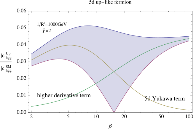
Figure 4: (color online). Contribution to the coupling $|c_{hgg}|$ (relative to the Standard Model) as a function of the Higgs localization parameter $\beta$ when considering only a five-dimensional up-type quark, and computed with the higher derivative term discussed in the text in addition to the standard 5D Yukawa coupling term. Since both contributions have independent phases we add and subtract their generic size to obtain the shaded region of possible values. These results are calculated by using only the first 3 KK modes (i.e. considering an effective theory with a cut-off of the order the the fourth KK mass). The dimensionless 5D Yukawas are fixed at $\tilde{Y}=2$ and the KK scale is set at $\displaystyle\frac{1}{R^{\prime}}=1000$ GeV (the overall effect scales as $\tilde{Y}^{2}v^{2}R^{\prime 2}$).

$\begin{array}[]{cc}\includegraphics[width=252.94499pt,height=199.16928pt]{RamanShiftTop.pdf}&\includegraphics[width=252.94499pt,height=199.16928pt]{RamanHggTop.pdf}\end{array}$

Figure 5: (color online). Shift of the top quark Yukawa coupling (left) and contribution to the coupling $c_{hgg}$ (right), relative to the Standard Model, as a function of the Higgs localization parameter $\beta$, when considering only a five-dimensional KK top quark, and including in the computation the higher derivative term discussed in the text, in addition to the standard 5D Yukawa coupling term. The contributions from each term have independent phases and so we add and subtract their absolute value to obtain the shaded region of possible values. These results are calculated by using only the first 3 KK modes (i.e. considering an effective theory with a cut-off of the order the the fourth KK mass). The values of the 5D Yukawa $Y^{u}$ and of $Y_{R}$ are fixed at $\tilde{Y}=2$ and the KK scale is set at $\frac{1}{R^{\prime}}=1000$ GeV (the overall effect scales as $\tilde{Y}^{2}v^{2}R^{\prime 2}$).

Its effects can therefore be tracked into the effects of these wrong chirality terms, as was already noted in the appendix of ATZ1 . We can thus formally treat the situation as before, where a truncated version of the infinite mass matrix of eq. (34) is considered (with just a few KK levels), but now we redefine the terms $Y^{u}_{U_{L}Q_{R}}$ to include the contributions from $Y_{R}$ as

$$Y_{U_{L}Q_{R}}^{u}=\int_{R}^{R^{\prime}}dz\left({R\over z}\right)^{5}\frac{v_{\beta}(z)}{v_{4}}\left(Y^{u}U_{L}(z)Q_{R}(z)+Y_{R}^{u}{z^{2}\over R^{2}}\partial_{z}U_{L}(z)\partial_{z}Q_{R}(z)\right).$$ (52)

It is now easy to compute numerically the new effects since from here we just have to repeat the previous procedure. The results are shown in Figures 4 and 5. In both figures we show the individual contributions coming from the normal Yukawa coupling $Y^{u}$, from the new $Y_{R}^{u}$ coupling, as well as the combined effect. This combined effect is represented by the shaded region, the reason being that the two types of couplings $Y^{u}$ and $Y_{R}^{u}$ have independent phases and so can add up constructively or destructively, or in between. In Figure 4 we focus on the contribution to $hgg$ due to an up-like 5D quark. In Figure 5 we show the predictions for the both shift in the SM top quark Yukawa coupling as well as the prediction for the contribution to the $hgg$ coupling coming from a 5D top-like quark. As we can see, the shift in the top quark Yukawa coupling can be quite large, and for low values of the Higgs localization parameter $\beta$ the shift obtained always results in a suppression in the Yukawa coupling. For large values of $\beta$ the shift can be in either direction (suppression or enhancement). In the case of the $hgg$ coupling, we see that the contribution represents an enhancement with respect to the SM prediction for small values of $\beta$, and again for large values of $\beta$ the $c_{hgg}$ coupling can be either enhanced or suppressed depending on the relative phases between $Y_{R}$ and $Y^{u}$. For this comparison we have taken the absolute value of both couplings $Y_{R}$ and $Y^{u}$ to be the same, i.e. $\tilde{Y}=2$, in appropriate units of the cutoff. The main feature to remember is that the effects of the higher derivative operator $Y_{R}$ are subdominant for small $\beta$ but become dominant for large $\beta$. The large contribution obtained at large $\beta$ is precisely what makes these new predictions consistent with the results obtained with the original infinite sum, and so the higher derivative operators that we have considered here somewhat encode the UV sensitivity found in the previous section.

VI Misalignment between Higgs VEV and Higgs profile

In this section we present a discussion on how to treat the case where the Higgs profile is different form its VEV profile. This is equivalent to consider the mixing effects between the massless zero mode Higgs boson, and the heavy KK Higgs modes and its effects on the Higgs observables computed in this paper.

We follow closely an argument by Azatov azatovhiggsvev and for simplicity we will discuss a simple situation in which the 4D effective theory contains only two new heavy vector-like fermions, $Q$ and $U$, doublet and singlet of $SU(2)_{L}$ respectively. This is the situation one would have when the KK fermion towers are truncated after the first KK excitation.

Let’s first define our notation for the following quantities

$$Y^{\beta}_{ij}\equiv\int dz\left(\frac{R}{z}\right)^{5}\psi_{i}\ \psi_{j}\frac{v_{\beta}(z)}{v_{4}}$$

$$X^{\beta}_{ij}\equiv\int dz\left(\frac{R}{z}\right)^{5}\psi_{i}\ \psi_{j}\ h_{\beta}(z),$$ (53)

where $v_{4}$ is the SM Higgs VEV and $v_{\beta}(z),h_{\beta}(z)$ are the 5D profiles of the Higgs VEV and the Higgs physical field, which are generically different. That is, after EWSB, the Higgs field is expanded around the nontrivial VEV $v_{\beta}(z)$ as

$$H(x,z)=v_{\beta}(z)+h(x)h_{\beta}(z)+...\,.$$ (54)

In the case of the bulk Higgs sector considered here, both profiles $v_{\beta}(z),h_{\beta}(z)$ are almost the same, (see eq. (14)), the order of the misalignment between them being controlled by powers of $(m_{h}R^{\prime})^{2}$ (a small quantity).

We consider all the possible couplings between the Higgs and the fermions of the effective theory which after EWSB can be written as the matrix ${\cal M}(v_{4},h)$ as

$$\left(\bar{q_{L}},\bar{Q_{L}}\bar{U_{L}}\right)\left(\begin{array}[]{ccc}Y^{\beta}_{q_{L}u_{R}}\ v_{4}+X^{\beta}_{q_{L}u_{R}}h(x)&0&Y^{\beta}_{q_{L}U_{R}}\ v_{4}+X^{\beta}_{q_{L}U_{R}}h(x)\\ Y^{\beta}_{Q_{L}u_{R}}\ v_{4}+X^{\beta}_{Q_{L}u_{R}}h(x)&M_{Q}&Y^{\beta}_{Q_{L}U_{R}}\ v_{4}+X^{\beta}_{Q_{L}U_{R}}h(x)\\ 0&Y^{\beta}_{U_{L}Q_{R}}\ v_{4}+X^{\beta}_{U_{L}Q_{R}}h(x)&M_{U}\end{array}\right)\left(\begin{array}[]{c}u_{R}\\ Q_{R}\\ U_{R}\end{array}\right),\ \ \ \ \$$ (61)

The coupling between the physical Higgs and the two gluons is controlled by the physical Yukawa couplings $Y^{\rm phys}_{i}$ and masses $M^{\rm phys}_{i}$ of the heavier physical fermions running in the loop (top quark and KK modes), i.e.

$$\sum_{\rm heavy}\frac{Y^{\rm phys}_{i}}{M^{\rm phys}_{i}}=Tr({\bf Y}_{\rm phys}{\bf M}_{\rm phys}^{-1})-\sum_{\rm light}\frac{y_{i}}{m_{i}},$$ (62)

where ${\bf Y}_{\rm phys}$ is the physical Yukawa coupling and ${\bf M}_{\rm phys}$ is the physical fermion mass matrix of the setup. Because the trace is invariant under unitary transformations, we can rotate to the gauge basis and write

$$Tr({\bf Y}_{\rm phys}{\bf M}_{\rm phys}^{-1})=Tr({\bf Y}_{\rm gauge}{\bf M}_{\rm gauge}^{-1}),$$ (63)

and note that we can now relate this to the matrix ${\cal M}(v_{4},h)$ as

$$Tr({\bf Y}_{\rm gauge}{\bf M}_{\rm gauge}^{-1})=\partial_{h}\log(Det{\cal M}(v_{4},h))|_{h=0}.$$ (64)

The procedure is the same as was followed in Section III, i.e. we compute the the determinant by expanding in powers of $v^{2}/M_{i}^{2}$ and after combining everything we obtain

$$\sum_{\rm heavy}\frac{Y_{i}^{\rm phys}}{M_{i}^{\rm phys}} = \partial_{h}\log Det{\cal M}(v_{4},h)-\frac{y^{\rm light}}{m^{\rm light}}$$ (65)

$$= v_{4}\left(-\frac{X^{\beta}_{Q_{L}U_{R}}Y^{\beta}_{U_{L}Q_{R}}}{M_{Q}M_{U}}-\frac{X^{\beta}_{U_{L}Q_{R}}Y^{\beta}_{Q_{L}U_{R}}}{M_{Q}M_{U}}\right).$$

This result is the equivalent to eq. (40) with the effect of the misalignment between $v_{\beta}(z)$ and $h_{\beta}(z)$. One sees that the difference lies in the substitution of one of the $Y$ terms by an $X$ term, and so the correction to the result of eq. (40) is

$$\delta{c_{hgg}}=v_{4}\left(-\frac{\left(X^{\beta}_{Q_{L}U_{R}}-Y^{\beta}_{Q_{L}U_{R}}\right)Y^{\beta}_{U_{L}Q_{R}}}{M_{Q}M_{U}}-\frac{\left(X^{\beta}_{U_{L}Q_{R}}-Y^{\beta}_{U_{L}Q_{R}}\right)Y^{\beta}_{Q_{L}U_{R}}}{M_{Q}M_{U}}\right),$$ (66)

which is controlled by

$$\left(X^{\beta}_{U_{L}Q_{R}}-Y^{\beta}_{U_{L}Q_{R}}\right)=\int dz\left(\frac{R}{z}\right)^{5}U_{L}(z)Q_{R}(z)\left(h_{\beta}(z)-\frac{v_{\beta}(z)}{v_{4}}\right),\ \ \ \ \$$ (67)

and

$$\left(X^{\beta}_{Q_{L}U_{R}}-Y^{\beta}_{Q_{L}U_{R}}\right)=\int dz\left(\frac{R}{z}\right)^{5}Q_{L}(z)U_{R}(z)\left(h_{\beta}(z)-\frac{v_{\beta}(z)}{v_{4}}\right),\ \ \ \ \$$ (68)

and since the misalignment between $v_{\beta}(z)$ and $h_{\beta}(z)$ can be computed perturbatively ATZ1 as

$$h_{\beta}(z)-\frac{v_{\beta}(z)}{v_{4}}=\frac{v_{\beta}(z)}{v_{4}}\left(\frac{m_{h}^{2}{R^{\prime}}^{2}}{2(4+\beta)}+\frac{m_{h}^{2}{z}^{2}}{4(1+\beta)}+{\cal O}(m_{h}^{4}{R^{\prime}}^{4})\right),$$ (69)

we obtain

$$\left(X^{\beta}_{U_{L}Q_{R}}-Y^{\beta}_{U_{L}Q_{R}}\right)=m_{h}^{2}{R^{\prime}}^{2}\left(\frac{Y^{\beta}_{U_{L}Q_{R}}}{2(4+\beta)}+\frac{Y^{\beta+2}_{U_{L}Q_{R}}}{4\sqrt{(1+\beta)(3+\beta)}}\right)+{\cal O}(m_{h}^{4}{R^{\prime}}^{4}).$$ (70)

In other words, the effect of considering the misalignment between $v_{\beta}(z)$ and $h_{\beta}(z)$ is to add a correction with the same structure as the result of eq. (40), but with a suppression of $\left(m_{h}{R^{\prime}}\right)^{2}$, i.e. the correction is at most ${\cal O}(1\%)$, and becomes much smaller for increasing values of $\beta$.

VII Discussion and Outlook

In this work we have presented the results for the predictions of Higgs phenomenology in a toy-model RS setup in which the Higgs field is allowed to propagate in the bulk and with a single 5D fermion field. Our results can be extended to three families to include full flavor effects, but the generic predictions that we would obtain are expected to be basically the same as the ones presented in ATZ1 ; ATZ2 . That is, that in the context of flavor anarchy, where the action parameters are all of the same order but with more or less random values and phases (with the constraint of obtaining correct SM predictions) the couplings of the Higgs with fermions and gluons and photons can receive important corrections, either enhancing or suppressing the SM predictions. However, the two references mentioned present calculations performed by including the effect of all the KK fermions, technically assuming an infinite cut-off for the model (where a brane Higgs is considered). In general, all these scenarios break down at a low cut-off, becoming strongly coupled for both gauge and Yukawa interactions. The implicit assumption made in ATZ1 ; ATZ2 was that the effects of the heavier modes should decouple quickly, at least for the case of a bulk Higgs field. The main motivation to perform the calculations by considering the full infinite fermion KK tower, as well as pushing the Higgs into the brane was mainly of technical nature. Indeed both the flavor structure of the Higgs Yukawa couplings as well as the coupling to gluons and photons can be computed analytically with those ingredients. In ATZ1 , the authors checked analytically that the corrections to the Higgs Yukawa couplings were actually of the same order for a bulk Higgs and a brane Higgs.

However it was pointed out in Neubert that in the brane Higgs case, the effects of the heavier KK fermion modes do not decouple and that they all contribute evenly in the computation of the Higgs couplings in the model. On the other hand, we showed in sections III and IV of this paper that the heavier KK modes in the case of a bulk Higgs do decouple very quickly, so that the analytical result obtained by using the infinite KK tower approaches with great precision the numerical result obtained by considering an effective theory with only a few KK fermion modes. Moreover, when considering the effective theory with only a few KK modes, one should include in the action all possible operators and in particular the higher derivative ones introduced in Section V. These effects were omitted in Neubert , and as we showed in this work, the importance of these operators increases as the Higgs is more and more localized towards the brane. In Bouchart:2009vq , the authors considered an RS setup with a highly localized Higgs and the presence of only a few KK fermions and studied the effects on the Higgs couplings to gluons and photons, among other observables. In the limit of the SM gauge group (they did consider an extended gauge group) they found no significant deviations from the SM predictions. Indeed this result is consistent with our findings of Section IV (no higher derivative operators invoked yet), since as it can be seen on Figures 5 and 4, the shift in Higgs Yukawa couplings and the new effects to Higgs-gluon-gluon coupling vanish in the limit of highly localized Higgs (large $\beta$ parameter). On the other hand, in Neubert it is claimed that large effects should be present in the case of a brane Higgs and with only a few KK modes present in the effective theory (and no higher derivative operators), a result inconsistent with both our findings and those found in Bouchart:2009vq . We can trace the origin of the disagreement in their calculation of the Higgs Yukawa couplings. Those are computed by using the full 5D equations of motion, which as we have said earlier is equivalent to considering the complete tower of KK modes. Then, using these couplings, they calculate the $hgg$ radiative coupling but now including only a finite amount of KK fermions. This treatment leads to a highly suppressed top quark Yukawa coupling (due to effects from the infinite KK tower) and a vanishing contribution to $hgg$ from the loops of KK fermions considered (one would need the whole tower to obtain a finite effect). Their end result is a suppressed top quark Yukawa coupling and a suppressed $hgg$ coupling (due to the smaller top quark Yukawa), predictions which are at odds with the findings of Bouchart:2009vq ; ATZ2 and of this paper.

The procedure of Neubert seems inconsistent because essentially the authors use infinite KK degrees of freedom in one part of their calculation (the SM quark Yukawa couplings computation via equations of motion) but then they truncate the KK degrees of freedom in order to compute the $hgg$ coupling. In any case, had they included the higher derivative operators introduced in this paper, their results would have changed dramatically since then, the effect to $hgg$ coming from the top quark Yukawa loop would remain basically the same, but the effects due to loops of a few KK fermions would dominate the overall effect (and thus the result would start to become consistent with the findings of ATZ2 ).

Also, the predictions of Bouchart:2009vq should change if one considers the effects of the higher derivative operators introduced in Section V. In that situation, the Higgs couplings can receive large corrections, and can be of any sign (suppression or enhancement) due to the different phases present in the couplings $Y$ and $Y_{R}$. In fact we have found here that for a Higgs field in the bulk, our results are more predictive than for a brane Higgs field, because the effect of the higher derivativer operators is subdominant for a bulk Higgs field. The effects from only the 5D Yukawa operators are aligned ATZ1 , and thus all the KK quarks add up in phase. In that situation we can have definite predictions for the effects caused by a single family of fermions, i.e. it will produce a suppression in the light quark Yukawa coupling and an enhancement in Higgs boson production (as well as suppression in the Higgs to photons coupling) ATZ2 , with the caveat of taking the dimensionless couplings of both Yukawa terms and higher derivative operators to be the same (consistent with the usual assumption that all 5D coefficients have to be of the same order). Taking into account the three fermion families in conjunction with a bulk Higgs field might weaken this prediction due to complicated flavor mixings and structure, but still one should be able to draw a correlation between Yukawa couplings and Higgs production (and $h\to\gamma\gamma$) for the case of a bulk Higgs field. The parameter space of the bulk Higgs scenario can therefore be under a tighter pressure as more and more precise experimental measurements in Higgs observables at the LHC become available. In particular if the predicted and correlated deviations of Higgs couplings is not clearly observed this should put bounds on the KK scale of the bulk Higgs scenario.

The situation for a Higgs on the brane is different. The higher order derivative terms are now important. Each KK tower of light quarks and the top will contribute to the $hgg$ coupling, but their effect depends on arbitrary relative phases (between $Y_{R}$ and $Y_{5d}$), and so one cannot make a firm statement about the magnitude and phase of the overall contribution: it can be a suppression or an enhancement, or in between.

Finally we comment again on the apparent problem of a highly localized Higgs scenario (brane Higgs) in which predictions made from a truncated fermion KK tower are very different from predictions made from an infinite fermion KK tower. This apparent UV-sensitivity can actually be lifted by considering the higher derivative operators described here (first introduced in ATZ1 ). When these are included, the predictions made with a finite KK fermion tower become consistent with the original predictions obtained with an infinite fermion tower. A more esthetic problem with the brane Higgs scenario remains, since the definition of the Higgs operators seems highly unnatural, if one understands a brane Higgs field as a limit of a bulk Higgs field. All operators involving Higgs fields will have to have a precise and definite dependence on $\beta$ (a large number), which seems quite contrived, specially in a framewrok in which no big numerical hierarchies should arise from fundamental 5D coefficients. In any case, with the ansatz outlined in the text and reviewed in Appendix B, one can still work consistently with a brane Higgs field as a limit case of a bulk Higgs field.

VIII Appendix

Appendix A Some Explicit Analytic Results

From equation (39) the shift defined as $\displaystyle\frac{\Delta}{m{v_{4}}}\equiv\frac{1}{{v_{4}}}-\frac{Y}{m}$, can be also derived from

$$\frac{\Delta}{m{v_{4}}}={{v_{4}}\over Y^{u}_{qu}}\sum_{i,j}{Y^{u}_{qU_{j}}Y^{u*}_{U_{j}Q_{i}}Y^{u}_{Q_{i}u}\over M_{Q_{i}}M_{U_{j}}}.$$ (71)

Therefore simply replacing the second Yukawa coupling with the Yukawa coupling of the Higher derivative operator, $Y^{R}$ will give

$$\frac{\Delta^{R}}{m{v_{4}}}={{v_{4}}\over Y^{u}_{qu}}\sum_{i,j}{Y^{u}_{qU_{j}}Y^{Ru*}_{U_{j}Q_{i}}Y^{u}_{Q_{i}u}\over M_{Q_{i}}M_{U_{j}}}.$$ (72)

Here, we present explicit analytic expressions for the $hgg$ production and also the Yukawa coupling-mass shifts by performing the infinite sums over the KK modes. We also include the result given in reference ATZ1 for the shift due to the usual Yukawa term, $Y_{d}\bar{Q}HU$, for completeness. To summarize, we have

$$c_{hgg} =\frac{2m_{d}^{2}}{{v_{4}}}R^{\prime 2}\frac{2+c_{u}-c_{q}+\beta}{(1-2c_{q})(1+2c_{u})}\left[\frac{(1-\epsilon^{1-2c_{q}})(1-\epsilon^{1+2c_{u}})}{4+2\beta}-\frac{1-\epsilon^{1-2c_{q}}}{5+2c_{u}+2\beta}-\frac{1-\epsilon^{1+2c_{u}}}{5-2c_{q}+2\beta}\right.$$ (73)

$$\left.+\frac{\epsilon^{1-2c_{q}}}{4+2\beta}(1-\epsilon^{1+2c_{u}})+\frac{\epsilon^{1+2c_{u}}}{4+2\beta}(1-\epsilon^{1-2c_{q}})+\frac{\epsilon^{2-2c_{q}+2c_{u}}}{2-c_{u}+c_{q}+\beta}-\frac{\epsilon^{-2c_{q}+1}}{3+c_{u}+c_{q}+\beta}-\frac{\epsilon^{1+2c_{u}}}{3-c_{u}-c_{q}+\beta}\right.$$

$$\left.+\frac{1}{4+c_{u}-c_{q}+\beta}\right]+{y_{t}^{RS}\over m_{t}}A_{1/2}(\tau_{t})+{\Delta_{2}^{t}\over m_{t}{v_{4}}}\,,$$

for the $hgg$ production and

$$\frac{\Delta^{d}_{1}}{m{v_{4}}} =\frac{2m_{d}^{2}}{{v_{4}}}R^{\prime 2}\frac{2+c_{u}-c_{q}+\beta}{(1-2c_{q})(1+2c_{u})}\left[\frac{(1-\epsilon^{1-2c_{q}})(1-\epsilon^{1+2c_{u}})}{6+c_{u}-c_{q}+3\beta}-\frac{1-\epsilon^{1-2c_{q}}}{5+2c_{u}+2\beta}-\frac{1-\epsilon^{1+2c_{u}}}{5-2c_{q}+2\beta}\right.$$ (74)

$$\left.+\frac{\epsilon^{1-2c_{q}}}{4+2\beta}(1-\epsilon^{1+2c_{u}})+\frac{\epsilon^{1+2c_{u}}}{4+2\beta}(1-\epsilon^{1-2c_{q}})+\frac{\epsilon^{2-2c_{q}+2c_{u}}}{2-c_{u}+c_{q}+\beta}-\frac{\epsilon^{-2c_{q}+1}}{3+c_{u}+c_{q}+\beta}-\frac{\epsilon^{1+2c_{u}}}{3-c_{u}-c_{q}+\beta}\right.$$

$$\left.+\frac{1}{4+c_{u}-c_{q}+\beta}\right]\,,$$

for the shifted Yukawa coupling. Also, there is a misalignment due to the kinetic term ATZ1 , which as discussed in the text, is only important for the case of the third generation quarks. We do not repeat that result here. For the higher derivative term the shift is:

$$\frac{\Delta^{d}_{R}}{m{v_{4}}} =2\frac{Y^{\prime}_{R}}{\Lambda^{2}}\frac{m_{d}^{2}}{{v_{4}}}\frac{2+c_{u}-c_{q}+\beta}{(1+2c_{u})(1-2c_{q})}\left[\frac{(4-c_{q}+\beta)(4+c_{u}+\beta)}{6+3\beta+c_{u}-c_{q}}(1-\epsilon^{1-2c_{q}})(1-\epsilon^{1+2c_{u}})\right.$$

$$\left.\ -\frac{(3-c_{q})(4-c_{q}+\beta)}{5+2\beta-2c_{q}}(1-\epsilon^{1+2c_{u}})-\frac{(3+c_{u})(4+c_{u}+\beta)}{5+2\beta+2c_{u}}(1-\epsilon^{1-2c_{q}})\right.$$

$$\left.\ +\frac{(2+c_{q})(4-c_{q}+\beta)}{4+2\beta}\epsilon^{1-2c_{q}}(1-\epsilon^{1+2c_{u}})+\frac{(2-c_{u})(4+c_{u}+\beta)}{4+2\beta}\epsilon^{1+2c_{u}}(1-\epsilon^{1-2c_{q}})\right.$$

$$\left.+\frac{(2+c_{q})(2-c_{u})}{2+c_{q}-c_{u}+\beta}\epsilon^{2-2c_{q}+2c_{u}}-\frac{(3-c_{q})(2-c_{u})}{3-c_{u}-c_{q}+\beta}\epsilon^{1+2c_{u}}-\frac{(2+c_{q})(3+c_{u})}{3+c_{u}+c_{q}+\beta}\epsilon^{1-2c_{q}}+\frac{(3-c_{q})(3+c_{u})}{4+c_{u}-c_{q}+\beta}\right].$$

Appendix B From Bulk to Brane

We summarize the matching prescription for operators containing Higgs field for the case where the Higgs boson is localized on the brane. As explained in Section II, these prescriptions insures that the 5D bulk Higgs scenario transitions smoothly to a brane-localized Higgs case. The brane prescription for the Higgs associates a delta function to the Higgs normalization integral

$$\int_{R}^{R^{\prime}}(\frac{R}{z})^{3}dz[h_{\beta}(z)]^{2}=1\,.$$

As the $HH$, rather than $H$ field, is associated with a $\delta$ function, one must include a $\beta$ dependence to the bulk Higgs fields to be able to match operators, in the limit $\beta\to\infty$ to the brane ones. The conversion is:

$$H\to\sqrt{\beta}\,,$$

$$HH\to HH\,,$$

$$HHH\to\frac{1}{\sqrt{\beta}}HHH\,,$$

for matching brane to bulk in the appropriate limit.

So for the shift, we have contributions from $Y_{2}$ and $Y_{R}$. As we are dealing with an effective theory, we look at the effect of summing over a finite number of modes, let’s say 3 to 5.

For the case of brane Higgs, the contributions for a finite number of modes for $Y_{2}$ give exactly $0$ (because of boundary values on the brane). This confirms the work of Bouchart:2009vq . However, we must add higher order operators $Y_{R}$, which give a significant result (converging to a constant for $\beta\to 1000$ and anything beyond). The result obtained by summing over a finite number of modes in the brane on the $Y_{R}$ contribution must be compared with the result in the paper by ATZ1 for the infinite sum of $Y_{2}$ on the brane.

For bulk Higgs, the shift contribution from a finite number of modes on the $Y_{2}$ contribution is no longer $0$. However, adding to this the $Y_{R}$ contribution, we notice that the $Y_{R}$ contribution for bulk Higgs is much smaller (two orders of magnitude) than the corresponding one in the brane. This is a clear indication that higher order corrections are much more important for the brane Higgs case than for the bulk.

References

- (1) L. Randall and R. Sundrum, Phys. Rev. Lett. 83, 3370 (1999); L. Randall and R. Sundrum, Phys. Rev. Lett. 83, 4690 (1999).
- (2) H. Davoudiasl, J. L. Hewett and T. G. Rizzo, Phys. Lett. B 473, 43 (2000); A. Pomarol, Phys. Lett. B 486, 153 (2000); S. Chang, J. Hisano, H. Nakano, N. Okada and M. Yamaguchi, Phys. Rev. D 62, 084025 (2000).
- (3) K. Agashe et al., Phys. Rev. D 71 (2005) 016002; D 75 (2007) 015002; D 74 (2006) 053011; Phys. Rev. Lett. 93 (2004) 201804; S. J. Huber and Q. Shafi, Phys. Lett. B 512 (2001) 365; B 544 (2002) 295; B 583 (2004) 293; T. Appelquist et al., Phys. Rev. D 65 (2002) 105019; T. Gherghetta, Phys. Rev. Lett. 92 (2004) 161601; G. Moreau et al., JHEP 0601 (2006) 048; 0603 (2006) 090; Eur. Phys. J. C 40 (2005) 539; S. Chang et al., Phys. Rev. D 73 (2006) 033002.
- (4) C. Csaki, A. Falkowski and A. Weiler, JHEP 0809, 008 (2008); [arXiv:0804.1954 [hep-ph]]. A. L. Fitzpatrick, G. Perez and L. Randall, arXiv:0710.1869 [hep-ph]. M. Blanke, A. J. Buras, B. Duling, S. Gori and A. Weiler, JHEP 0903, 001 (2009) [arXiv:0809.1073 [hep-ph]]; M. Blanke, A. J. Buras, B. Duling, K. Gemmler and S. Gori, JHEP 0903, 108 (2009) [arXiv:0812.3803 [hep-ph]]; M. E. Albrecht, M. Blanke, A. J. Buras, B. Duling and K. Gemmler, JHEP 0909, 064 (2009) [arXiv:0903.2415 [hep-ph]]; M. Bauer, S. Casagrande, L. Grunder, U. Haisch and M. Neubert, Phys. Rev. D 79, 076001 (2009) [arXiv:0811.3678 [hep-ph]]; M. Bauer, S. Casagrande, U. Haisch and M. Neubert, arXiv:0912.1625v1 [hep-ph].
- (5) G. Cacciapaglia, C. Csaki, J. Galloway, G. Marandella, J. Terning and A. Weiler, JHEP 0804, 006 (2008); A. L. Fitzpatrick, L. Randall and G. Perez, Phys. Rev. Lett. 100, 171604 (2008); J. Santiago, JHEP 0812, 046 (2008); C. Csaki, G. Perez, Z. Surujon and A. Weiler, Phys. Rev. D 81, 075025 (2010); M. C. Chen, K. T. Mahanthappa and F. Yu, Phys. Rev. D 81, 036004 (2010); M. C. Chen and H. B. Yu, Phys. Lett. B 672, 253 (2009); G. Perez and L. Randall, JHEP 0901, 077 (2009); C. Csaki, C. Delaunay, C. Grojean and Y. Grossman, JHEP 0810, 055 (2008) [arXiv:0806.0356 [hep-ph]]; F. del Aguila, A. Carmona and J. Santiago, arXiv:1001.5151 [hep-ph]. C. Csaki, A. Falkowski and A. Weiler, Phys. Rev. D 80, 016001 (2009) [arXiv:0806.3757 [hep-ph]].
- (6) J.A. Cabrer, G. von Gersdorff, and M. Quiros, New J. Phys. 12 (2010) 075012; J.A. Cabrer, G. von Gersdorff, and M. Quiros, Phys. Rev. D 84 (2011) 035024; J.A. Cabrer, G. von Gersdorff, and M. Quiros, JHEP 1105 (2011) 083; A. Carmona, E. Ponton and J. Santiago, JHEP 1110 (2011) 137; P. R. Archer, J.S. Huber and S.Jager, JHEP bf 1112(2011), 101.
- (7) R. Contino, Y. Nomura and A. Pomarol, Nucl. Phys. B 671, 148 (2003), K. Agashe, R. Contino and A. Pomarol, Nucl. Phys. B 719, 165 (2005).
- (8) G. F. Giudice, C. Grojean, A. Pomarol and R. Rattazzi, JHEP 0706, 045 (2007) [arXiv:hep-ph/0703164].
- (9) I. Low, R. Rattazzi and A. Vichi, JHEP 1004, 126 (2010) [arXiv:0907.5413 [hep-ph]].
- (10) ATLAS Collaboration, arXiv:1207.7214 [hep-ex]; CMS Collaboration, arXiv:1207.7235 [hep-ex].
- (11) K. Agashe, A. Azatov, and L. Zhu, Phys. Rev. D 46 (2009) 056006.
- (12) B. Lillie, JHEP 0602, 019 (2006) [arXiv:hep-ph/0505074].
- (13) A. Falkowski, Phys. Rev. D 77, 055018 (2008) [arXiv:0711.0828 [hep-ph]].
- (14) A. Djouadi and G. Moreau, Phys. Lett. B 660, 67 (2008) [arXiv:0707.3800 [hep-ph]].
- (15) G. Cacciapaglia, A. Deandrea and J. Llodra-Perez, JHEP 0906, 054 (2009) [arXiv:0901.0927 [hep-ph]].
- (16) C. Bouchart and G. Moreau, Phys. Rev. D 80, 095022 (2009) [arXiv:0909.4812 [hep-ph]].
- (17) S. Casagrande, F. Goertz, U. Haisch, M. Neubert, and T. Pfoh, JHEP 0810 (2008) 094; JHEP 1009 (2010) 017, M. Carena, S. Casagrande, F. Goertz, U. Haisch and M. Neubert, JHEP 1208, 156 (2012) [arXiv:1204.0008 [hep-ph]].
- (18) A. Azatov, M. Toharia, and L. Zhu, Phys. Rev. D 82, 056004 (2010).
- (19) J. Gunion, H. Haber, G. Kane, and S. Dawson, The Higgs Hunter’s Guide (Westview press, Boulder, CO, 2000).
- (20) A. Azatov, M. Toharia, and L. Zhu, Phys. Rev. D 80, 035016 (2009).
- (21) K. Agashe, A. E. Blechman and F. Petriello, Phys. Rev. D 74, 053011 (2006) [hep-ph/0606021].
- (22) G. Cacciapaglia, C. Csaki, G. Marandella and J. Terning, JHEP 0702, 036 (2007), [arXiv:hep-ph/0611358].
- (23) A. Azatov, private communication (2012).
- (24) J. Hirn and V. Sanz, Phys, Rev. D 76, 044022 (2007).
- (25) See for example E. M. Lifshitz, V. B. Berestetskii, L. P. Pitaevskii, Quantum Electrodynamics, 2nd ed. (Pergamon Press, 1982).