Linearized gravitational waves near space-like and null infinity

Abstract

Linear perturbations on Minkowski space are used to probe numerically the remote region of an asymptotically flat space-time close to spatial infinity. The study is undertaken within the framework of Friedrich’s conformal field equations and the corresponding conformal representation of spatial infinity as a cylinder. The system under consideration is the (linear) zero-rest-mass equation for a spin-2 field. The spherical symmetry of the underlying background is used to decompose the field into separate non-interacting multipoles. It is demonstrated that it is possible to reach null-infinity from initial data on an asymptotically Euclidean hyper-surface and that the physically important radiation field can be extracted accurately on $\mathscr{I}^{+}$.

1 Introduction

Asymptotically simple space-times as defined by Penrose Penrose:1965wj are distinguished by their qualitatively completely different structure at infinity. Depending on the sign of the cosmological constant $\lambda$ their conformal boundary is time-like, space-like or null. These space-times have been studied extensively from the point of view of the initial (boundary) value problem and a lot is known about their properties. In particular, space-times which are asymptotically de Sitter ($\lambda>0$) are known to exist globally for small initial data. The same is true for asymptotically flat space-times ($\lambda=0$) while for asymptotically anti-de Sitter space-times we only have short-time existence results for the initial boundary value problem. On the contrary, initiated by an important paper by Bizoń and Rostrowroski Bizon:2011kz and based on numerical and perturbative methods, there are now strong hints that these space-times are in fact non-linearly unstable (for more details on this topic see the contribution by O. Dias in this volume).

In the present paper we want to focus on asymptotically flat space-times. As we already mentioned these space-times exist globally for small enough initial data. However, it is still not completely understood in detail, how to characterize the admissible initial data from a geometrical or physical point of view. The reason lies in the fact that in every space-time with a non-vanishing ADM-mass spatial infinity is necessarily singular for the 4-dimensional conformal structure.

In a seminal paper Friedrich:1998tc , Friedrich shows how to set up a particular gauge near space-like infinity which exhibits explicitly the structure of the space-time near space-like and null-infinity. The so called ‘conformal Gauß gauge’ is based entirely on the conformal structure of the space-time fixing simultaneously a coordinate system, an orthogonal frame and a general Weyl connection compatible with the conformal structure. The detailed description of this gauge is beyond the scope of this paper and we need to refer the reader to the existing literature Friedrich:1995uf ; Friedrich:1987ul ; Friedrich:1998tc ; Frauendiener:2004te . Suffice it to say that the conformal Gauß gauge is based on a congruence of time-like conformal geodesics emanating orthogonally from an initial space-like hyper-surface. The coordinate system, tetrad and Weyl connection are defined initially on that hyper-surface and are dragged along the congruence of conformal geodesics so that they are defined everywhere.

It turns out that in this gauge the space-time region near space-like infinity has a boundary consisting of future and past null-infinity $\mathscr{I}^{\pm}$ together with a 3-dimensional ‘cylindrical’ hyper-surface $I$ connecting them. In a certain sense, in Minkowski space-time, this cylinder is a blow-up of the (regular) point $i^{0}$. The ‘general conformal field equations’ (GCFE) express the fact that the conformal class of the space-time contains an Einstein metric. They are a set of geometric partial differential equations (PDEs) generalizing the standard Einstein equations with cosmological constant. When split into evolution and constraint equations within the conformal Gauß gauge the evolution equations take a particularly simple form and it turns out that the cylinder $I$ becomes a total characteristic. This means that the evolution equations reduce to an intrinsic system of PDEs on $I$, i.e., they contain no derivatives transverse to $I$. The intrinsic equations are symmetric hyperbolic on $I$ except for the locations $I^{\pm}:=I\cap\mathscr{I}^{\pm}$, the 2-spheres where $I$ meets future or past null-infinity. There, the equations loose hyperbolicity. It is this feature which is responsible for the singular behavior of the conformal structure near space-like infinity.

In a series of papers Friedrich:2008gs ; Friedrich:1998tc ; Friedrich:2008wt ; Friedrich:2007vc , Friedrich has analyzed the behavior of the fields, in particular of the Weyl tensor components and their transverse derivatives, along the cylinder $I$. He has shown that generic initial data lead to singularities at $I^{\pm}$. The singularities can be avoided if the initial data satisfy certain conditions, one of them being the geometric condition that the Cotton tensor of the induced geometry on the initial hyper-surface and all its symmetric trace-free derivatives vanish at the intersection of $I$ and the initial hyper-surface. It is still not completely clear what is the correct geometric classification of those space-times which satisfy Friedrich’s conditions (however, see Friedrich:2007vc ; Friedrich:2008wt ; Friedrich:2012vc ).

Here, we want to discuss these issues from the numerical point of view. It is clear, that the fact that the evolution equations extracted from the GCFE cease to be hyperbolic is a troublesome feature in a numerical evolution scheme. We want to see how it manifests itself in the simplest scenario we can think of: linearized gravitational fields on Minkowski space. If we could not control this situation then the use of the GCFE for numerical purposes would not be possible.

The plan of the paper is as follows: in Sect. 2 and Sect. 3 we give brief summaries of the basic analytical and numerical results. In Sect. 4 we discuss ways to overcome the singular behavior at $I^{+}$ while in Sect. 5 we show how we can reach future null-infinity. The conventions we use and much of the background can be found in Penrose:1984wm .

2 The spin-2 zero-rest-mass equations

It is well known Penrose:1984wm that perturbations of the Weyl tensor $C_{abc}{}^{d}$ or, equivalently, the Weyl spinor $\Psi_{ABCD}$ satisfy the equations for a field with spin 2 and vanishing rest-mass:

$$\nabla^{A}{}_{A^{\prime}}\phi_{ABCD}=0.$$ (1)

It is also known Penrose:1984wm that this system of equations suffers from Buchdahl conditions, algebraic conditions relating the conformal curvature $\Psi_{ABCD}$ of the underlying background geometry with the field

$$\Psi_{ABC(D}\phi^{ABC}{}_{E)}=0$$

which severely restrict the possible perturbations in any conformally curved space-time, rendering (1) inconsistent.

Therefore, we choose flat Minkowski space-time as our background so that $\phi_{ABCD}$ describes small amplitude gravitational waves propagating in an otherwise empty space-time. For a detailed discussion and derivation of the explicit form of the spin-2 equations in the present context we refer to Beyer:2012ie . Here, we focus only on the relevant points. Starting with the standard Minkowski metric in Cartesian coordinates $X^{\mathbf{a}}$

$$\tilde{g}=\eta_{\mathbf{a}\mathbf{b}}\mathrm{d}X^{\mathbf{a}}\mathrm{d}X^{\mathbf{b}}$$ (2)

where $\eta_{\mathbf{a}\mathbf{b}}=\mathrm{diag}(1,-1,-1,-1)$, and performing an inversion at the null-cone of the origin

$$X^{\mathbf{a}}=-\frac{x^{\mathbf{a}}}{x\cdot x},\qquad x\cdot x:=\eta_{\mathbf{a}\mathbf{b}}x^{\mathbf{a}}x^{\mathbf{b}}=\frac{1}{(X\cdot X)}$$

puts the metric into the form

$$\tilde{g}=\frac{\eta_{\mathbf{a}\mathbf{b}}\mathrm{d}x^{\mathbf{a}}\mathrm{d}x^{\mathbf{b}}}{(x\cdot x)^{2}}.$$ (3)

This metric is singular whenever $x\cdot x=0$, i.e., on the null-cone at infinity. So we define a conformally related metric

$$g^{\prime}=\Omega^{2}\tilde{g}=\eta_{\mathbf{a}\mathbf{b}}\mathrm{d}x^{\mathbf{a}}\mathrm{d}x^{\mathbf{b}},\qquad\Omega=-(x\cdot x)$$ (4)

which extends smoothly to the null-cone of infinity. Note, that space-like infinity is represented in this metric as the point $x^{\mathbf{a}}=0$. In order to exhibit the cylindrical structure referred to above we perform a further rescaling of the metric using a function $\kappa(r)=r\mu(r)$, where $r^{2}=(x^{1})^{2}+(x^{2})^{2}+(x^{3})^{2}$ and $\mu$ is a smooth function with $\mu(0)=1$. Furthermore, we introduce a new time coordinate by defining $x^{0}=t\kappa(r)$. These steps give the final form of the metric

$$g=\frac{1}{\kappa^{2}}\left(\kappa^{2}\mathrm{d}t^{2}+2t\kappa\kappa^{\prime}\mathrm{d}t\mathrm{d}r-(1-t^{2}\kappa^{\prime}{}^{2})\mathrm{d}r^{2}-r^{2}\mathrm{d}\omega^{2}\right).$$ (5)

Here, we have denoted the metric on the unit sphere by $\mathrm{d}\omega^{2}$. Note, that the metric $g$ is spherically symmetric.

The function $\mu(r)$ determines the ‘shape’ of $\mathscr{I}^{\pm}$ in the $(t,r)$-coordinate system. We have chosen the two possibilities $\mu(r)=1/(1+nr)$ with either $n=0$ or $n=1$ with the consequence that $\mathscr{I}^{\pm}$ are represented as either a horizontal ($n=0$) or diagonal ($n=1$) line in a $(t,r)$ diagram, see Fig. 1. They meet the cylinder $I$ in the spheres $I^{\pm}$ at $(t,r)=(\pm 1,0)$.

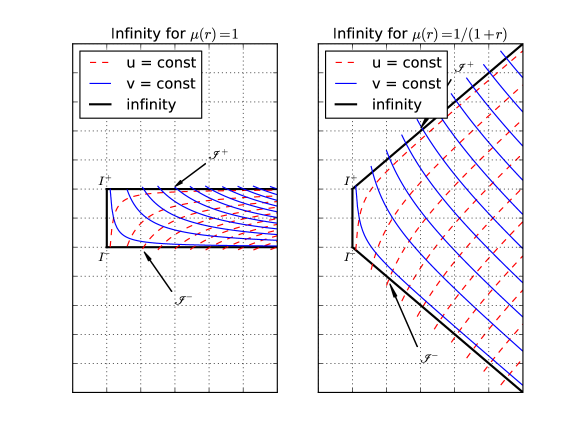
Figure 1: The neighborhood of space-like infinity in two different $(t,r)$-coordinate representations corresponding to $\mu(r)=1$ and $\mu(r)=1/(1+r)$

We introduce the double null-coordinates $(u,v)$ by

$$u=\kappa t-r,\qquad v=\kappa t+r,$$ (6)

which puts the metric into the form

$$g=\frac{1}{\kappa^{2}}\mathrm{d}u\mathrm{d}v-\frac{1}{\mu^{2}}\mathrm{d}\omega^{2}.$$

Null-infinity is characterized by the vanishing of one of the null coordinates, the other one being non-zero ($u=0$, $v\neq 0$ on $\mathscr{I}^{+}$ and $u\neq 0$, $v=0$ on $\mathscr{I}^{-}$). Both coordinates vanish on the cylinder $I$. In Fig. 1 we also display the lines of constant $u$ and $v$, corresponding to radial null geodesics. There are two families of null geodesics, one leaving the space-time through $\mathscr{I}^{+}$, the other entering it through $\mathscr{I}^{-}$.

Since the null coordinates are adapted to the conformal structure, we can see clearly that the cylinder is ‘invisible’ from the point of view of the conformal structure. This structure is exactly the same as the representation of space-like infinity in the coordinates $x^{\mathbf{a}}$, it appears like a point. However, the differentiable structures defined by the $(u,v)$ and the $(t,r)$ coordinates are completely different near the boundary $r=0$ from the one defined by the $x^{\mathbf{a}}$ coordinates.

In order to derive the spin-2 equations explicitly we introduce a complex null tetrad $(l^{a},n^{a},m^{a},\bar{m}^{a})$ adapted to the spherical symmetry, i.e.,

$$l^{a}\partial_{a}=\frac{1}{\sqrt{2}}\left(\left(1-t\kappa^{\prime}\right)\partial_{t}+\kappa\partial_{r}\right),\qquad n^{a}\partial_{a}=\frac{1}{\sqrt{2}}\left(\left(1+t\kappa^{\prime}\right)\partial_{t}-\kappa\partial_{r}\right),$$

and $m^{a}$ tangent to the spheres of symmetry. Writing the spin-2 equation in the NP formalism, computing the spin-coefficients and finally introducing the ‘eth’ operator $\eth$ (see Goldberg:1967tf ; Newman:1968tv ; Penrose:1984wm ) on the unit sphere puts (1) into the form of eight coupled equations

$$(1-t\kappa^{\prime})\partial_{t}\phi_{k}+\kappa\partial_{r}\phi_{k}-(3\kappa^{\prime}-(5-k)\mu)\phi_{k} =\mu\eth^{\prime}\phi_{k-1}, k=1:4,$$ (7)

$$(1+t\kappa^{\prime})\partial_{t}\phi_{k}-\kappa\partial_{r}\phi_{k}+(3\kappa^{\prime}+(k+1)\mu)\phi_{k} =\mu\eth\phi_{k+1}, k=0:3$$

for the five complex components of the spin-2 field $\phi_{ABCD}$, see e.g. Penrose:1984wm . We exploit the spherical symmetry of the background Minkowski space-time even further by decomposing the field components $\phi_{k}(t,r,\theta,\phi)$ into different multipole moments using the spin-weighted spherical harmonics ${}_{s}Y_{lm}$

$$\phi_{k}(t,r,\theta,\phi)=\sum_{l\geq 2-k}\sum_{m=-l}^{l}\phi^{lm}_{k}(t,r)\;{}_{2-k}Y_{lm}(\theta,\phi).$$ (8)

Inserting this expansion into (7) and using the action of $\eth$ and $\eth^{\prime}$ on the spin-weighted spherical harmonics Penrose:1984wm the system decouples into a countable family of $1+1$ systems indexed by admissible pairs of integers $(l,m)$. We find that each mode $\phi_{k}^{lm}$ propagates along radial null geodesics, the ‘inner’ modes $\phi_{1}^{lm}$, $\phi_{2}^{lm}$, $\phi_{3}^{lm}$ propagate in both directions while the ‘outer’ modes $\phi_{0}^{lm}$ and $\phi_{4}^{lm}$ only propagate along one null direction.

The final step in the preparation of the equations is the split into constraint and evolution equations, which leads to a system of five evolution equations

$$(1+t\kappa^{\prime})\partial_{t}\phi_{0}-\kappa\partial_{r}\phi_{0} =-(3\kappa^{\prime}-\mu)\phi_{0}-\mu\alpha_{2}\phi_{1},$$ (9)

$$\partial_{t}\phi_{1} =-\mu\phi_{1}+\frac{1}{2}\mu\alpha_{2}\phi_{0}-\frac{1}{2}\mu\alpha_{0}\phi_{2},$$

$$\partial_{t}\phi_{2} =\frac{1}{2}\mu\alpha_{0}\phi_{1}-\frac{1}{2}\mu\alpha_{0}\phi_{3},$$

$$\partial_{t}\phi_{3} =\mu\phi_{3}+\frac{1}{2}\mu\alpha_{0}\phi_{2}-\frac{1}{2}\mu\alpha_{2}\phi_{4},$$

$$(1-t\kappa^{\prime})\partial_{t}\phi_{4}+\kappa\partial_{r}\phi_{4} =(3\kappa^{\prime}-\mu)\phi_{4}+\mu\alpha_{2}\phi_{3}$$

and three constraint equations

$$-2\kappa\partial_{r}\phi_{1}+6r\mu^{\prime}\phi_{1}-2t\kappa^{\prime}\mu\phi_{1}+\alpha_{0}\mu(1-t\kappa^{\prime})\phi_{2}+\alpha_{2}\mu(1+t\kappa^{\prime})\phi_{0} =0,$$ (10)

$$-2\kappa\partial_{r}\phi_{2}+6r\mu^{\prime}\phi_{2}+\alpha_{0}\mu(1-t\kappa^{\prime})\phi_{3}+\alpha_{0}\mu(1+t\kappa^{\prime})\phi_{1} =0,$$

$$-2\kappa\partial_{r}\phi_{3}+6r\mu^{\prime}\phi_{3}+2t\kappa^{\prime}\mu\phi_{3}+\alpha_{0}\mu(1+t\kappa^{\prime})\phi_{2}+\alpha_{2}\mu(1-t\kappa^{\prime})\phi_{4} =0.$$

Note that we have dropped here the superscripts from $\phi_{k}^{lm}$ and we introduced the quantities $\alpha_{0}=\sqrt{l(l+1)}$ and $\alpha_{2}=\sqrt{l(l+1)-2}$. Since $\kappa(0)=0$ it is obvious that the evolution equations reduce to a system intrinsic to $I$. Since on $I$ also $\kappa^{\prime}(0)=1$, it follows that the coefficients in front of the time derivatives of $\phi_{0}$ (respectively $\phi_{4}$) vanish when $t=-1$ (respectively when $t=1$).

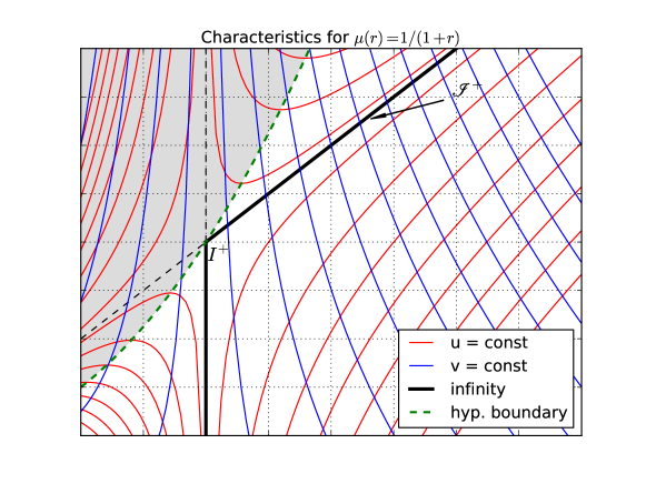
Figure 2: The characteristics of the evolution equations in a neighborhood of $I^{+}$ in the diagonal representation. The shaded region is the domain where the equations fail to be hyperbolic, i.e., where $t<\kappa^{\prime}(r)$. The corresponding neighborhood of $I^{-}$ is obtained by reflection at the lower border of the diagram accompanied by an interchange of $u$ and $v$. The thick (green) broken line indicates the boundary of the domain of non-hyperbolicity.

In Fig. 2 we show again the neighbourhood of $I$ and $\mathscr{I}^{+}$ for $\mu(r)=1/(1+r)$. This time we show the characteristics also in the unphysical part of the diagram. The non-shaded region bounded partly by the thick broken line is the domain of hyperbolicity of the evolution equations, i.e., the domain where $t<\pm|\kappa^{\prime}(r)|$. Notice that every neighborhood of $I^{+}$ contains regions where the hyperbolicity breaks down. Apart from the fact that one cannot hope to get existence and uniqueness of solutions beyond that region its presence also makes the numerical evolution challenging. For instance, setting up an initial boundary value problem with the left boundary at negative values of $r$ does not make sense if the evolution is to reach up to $I^{+}$. Even with the left boundary on $I$ it is not possible to go beyond $I^{+}$ since the evolution hits the non-hyperbolicity region.

3 Numerical methods and tests

Again, we give a brief summary and refer to Beyer:2012ie for further details. We have different equations for different values of the multipole index $l$. Here, we focus only on the case $l=2$ without mentioning it any further. We have done evolutions with other values of $l$ which lead to very similar results. The evolution equations (9) are solved on a spatial interval $0\leq r\leq 1$ as an initial boundary value problem. We use the method of lines constructing the spatial discretisation using a $4^{\text{th}}$ order accurate finite difference scheme. The initial data are obtained either from exact solutions or by solving the constraint equations (10) explicitly in terms of two free functions. The boundary at $r=0$ is a characteristic so we do not need to specify any free functions there, while the boundary at $r=1$ is an artificial boundary, which needs exactly one free function for the component $\phi_{0}$ that propagates through this boundary into the computational domain. The boundary conditions are implemented using SBP operators Strand:1994ef ; Gustafsson:1995vp ; Diener:2007bx and the SAT penalty method Carpenter:1994cu ; Carpenter:1999cl ; Lehner:2005hc ; Schnetter:2006ku . The semi-discrete system of ODEs is solved using the standard $4^{\text{th}}$ order Runge-Kutta method.

This code stably propagates the initial data from $t=0$ up to any value of $t<1$, independently of whether we use the diagonal or the horizontal representation of $\mathscr{I}$. The code converges to $4^{\text{th}}$ order, the constraints propagate and the constraint violations remain bounded. However, the two representations behave differently when we attempt to reach $t=1$.

In the diagonal case we can reach $t=1$ exactly and the code converges in $4^{\text{th}}$ order, indicating that the numerical problem is still well-posed. With any fixed time-step $\tau$ we can also step beyond $t=1$ to $t=1+\tau$. However, the code fails to converge at $t=1+\tau$ for every $\tau>0$. Clearly, the loss of hyperbolicity at $t=1$ is also responsible for the lack of well-posedness of the numerical problem. Referring back to Fig. 2 it is clear that there will always be a sufficiently high resolution in time and space which will detect the domain of non-hyperbolicity of the evolution equations beyond $I^{+}$.

In the horizontal case the situation is apparently worse. In this case, it is principally impossible to reach $t=1$ simply because the propagation speed of $\phi_{4}$ becomes infinite and so stability is lost not only at the point $I^{+}$ but at the entire time-slice $t=1$ which coincides with $\mathscr{I}^{+}$, a characteristic hyper-surface, in this representation.

However, in principle we can come arbitrarily close to $t=1$ (within numerical accuracy) if at every time we choose the next time-step small enough so that the CFL criterion—the numerical domain of dependence includes the analytical domain of dependence—is satisfied. Such an adaptive time-stepping scheme has been implemented and we have in fact demonstrated that we can come very close to $t=1$ without loosing convergence. However, since the time-steps decrease to zero exponentially with the number of steps the simulation takes arbitrarily long.

4 Beyond $I^{+}$?

Given that we can reach $t=1$ in a stable fashion in the diagonal representation we may ask the question as to whether it is possible to continue beyond $I^{+}$? Clearly, for the reasons discussed above we cannot simply continue the computation because we run into the non-hyperbolicity region near $I^{+}$. Referring back to Fig. 2 we see that one family of the characteristics—corresponding to the field component $\phi_{4}$—asymptotes to the cylinder and, subsequently, to $\mathscr{I}^{+}$ in a non-uniform way. This non-uniformity is due to the fact that the coefficient in front of the time derivative of $\phi_{4}$ in the evolution system vanishes at $t=1$, causing the loss of hyperbolicity of the system. Can we avoid this problem? There are a few possibilities which come to mind:

• Chop the computational domain by dropping points outside $\mathscr{I}^{+}$ from the left.

• Change the radial coordinate so that $\mathscr{I}^{+}$ becomes the left boundary of the computational domain. This is a form of $\mathscr{I}$-freezing (see Frauendiener:1998th ).

• Change the time coordinate so that the (space-like) time-slices tilt upwards towards $\mathscr{I}^{+}$.

We have considered the first two possibilities. These two methods are complementary to each other in the sense that in the first case we change the computational domain but not the system, while in the second case we change the equations but not the computational domain.

Fig. 2 shows the behavior of the characteristics for $\phi_{0}$ and $\phi_{4}$ as well as the region in which hyperbolicity fails. The surfaces that we are evolving our data on are horizontal and to the right of the vertical solid and broken black lines. Note that for $t>1$ these surfaces are guaranteed to intersect the region in which hyperbolicity fails. In addition, for surfaces with $t>1$ a new boundary condition for $\phi_{4}$, on the ‘left’ of the grid is required. However, since $\mathscr{I}^{+}$ is one of the characteristics for $\phi_{4}$ this boundary condition cannot influence the physical region to the right of $\mathscr{I}^{+}$.

To solve both of these problems we set the values of $\phi_{0},\ldots,\phi_{4}$ to zero after some predetermined grid point that is beyond future null infinity, but before the region in which hyperbolicity fails. That is, between the broken green line and $\mathscr{I}^{+}$. The equation for the broken green line is

$$1-\frac{t}{(r+1)^{2}}=0$$

and the equation for future null infinity, where $t\geq 1$, is

$$1-\frac{t}{r+1}=0.$$

We chose, after some experimentation, that the ‘cut off’ point, after which all data values would be set to zero would be $10\%$ of all grid points beyond $\mathscr{I}^{+}$. That is, the values of $\phi_{0},\ldots,\phi_{4}$ would be set to zero on the $90\%$ of grid points between $r=0$ and $\mathscr{I}^{+}$. This condition, of setting values to zero, allows us to numerically provide the necessary boundary condition for $\phi_{4}$ and cope with the lack of hyperbolicity in the region of the grid to the left of the broken green line.

Other than this technicality, the same evolution scheme, with the same fixed step size was used to evaluate the initial data up to $t=1.1$. We evolved an exact solution and estimated the error at $t=1.1$ by comparing the values of $\phi_{0},\ldots,\phi_{4}$, on the ‘physical’ portion of the grid to the exact solution. The $L_{2}$ measure of the error is presented in Table 1. We only give the error for the $\phi_{0}$ and $\phi_{4}$ components. The convergence rates for $\phi_{1},\phi_{2}$ and $\phi_{3}$ are, roughly, a linear interpolation between those for $\phi_{0}$ and $\phi_{4}$. Note, that the error in $\phi_{0}$ is of the order of $10^{-11}$ while the error in $\phi_{4}$ is roughly $10^{-2}$.

	$\phi_{0}$		$\phi_{4}$
Grid Points	$\log_{2}(||\Delta||_{2})$	Rate	$\log_{2}(||\Delta||_{2})$	Rate
100	-28.38		-5.93
200	-31.75	3.37	-5.98	0.05
400	-35.21	3.46	-6.07	0.10
800	-38.71	3.50	-8.41	2.34

Table 1: Absolute error $\Delta$ compared to an exact solution. $L^{2}$ norm and convergence rates at time $t=1.1$ for $\phi_{0},\phi_{4}$. The calculation was done with a fixed time-step.

In the second case we change the $r$-coordinate in a very simple minded way using the coordinate transformation

$$r\mapsto\bar{r}=r-t+1,\qquad t\mapsto\bar{t}=t,\qquad\text{for }t\geq 1.$$

This has the effect that $\mathscr{I}^{+}$ is given as the locus $\{\bar{r}=0\}$. Note, that the coordinate transformation is only continuous and not even $\mathcal{C}^{1}$. Since the partial derivatives transform according to

$$\partial_{t}=\partial_{\bar{t}}-\partial_{\bar{r}},\qquad\partial_{r}=\partial_{\bar{r}}$$

we still have the problem that the coefficient in front of the time derivative of $\phi_{4}$ vanishes at $t=1$. Clearly, we cannot make the system regular at $t=1$ by a coordinate transformation. We can try to avoid the evaluation at $t=1$ by arranging the time stepping to ‘straddle’ $t=1$ so that we never actually hit it exactly. However, this has the consequence that the ‘kink’ that we obtain due to the non-smoothness of the coordinate transformation induces oscillations at the right boundary. We would probably be able to avoid those if we used a smoother coordinate transformation. However, this would change the equations in much more complicated ways and we have not pursued this any further.

The third possibility mentioned above—changing the time coordinate—has the effect that the time-slices globally approach $\mathscr{I}^{+}$ which is exactly the feature that we see in the horizontal representation. This prompted us to look at the relationships between the different conformal representations in more detail.

The two representations are related by a conformal rescaling and a coordinate transformation. We can derive the corresponding relationships for the field components as follows. Let $\mu_{n}(r)=1/(1+nr)$ and define $\Theta=\mu_{1}/\mu_{0}$. Let $g_{0}$ and $g_{1}$ be the metrics corresponding to the horizontal and diagonal representations, then we have

$$g_{1}=\frac{\mu_{1}^{2}}{\mu_{0}^{2}}\,g_{0}=\Theta^{2}g_{0}.$$ (11)

Furthermore, the two time coordinates $t_{0}$ and $t_{1}$ in the two representations are related by

$$x^{0}=r\mu_{0}t_{0}=r\mu_{1}t_{1}\implies t_{1}=\Theta^{-1}t_{0}.$$ (12)

The spin-2 field has conformal weight $-1$ under conformal rescalings. This implies that with (11) we also have

$$\phi^{1}_{ABCD}=\Theta^{-1}\phi^{0}_{ABCD}.$$ (13)

In order to get the behavior of the field components under conformal rescalings we observe that (11) implies that the tetrad vectors rescale as

$$l^{a}_{1}=\Theta^{-1}l^{a}_{0},\quad\text{etc}$$ (14)

and the spin-frame correspondingly rescales with $\Theta^{-1/2}$. Taken altogether, these transformation properties imply that

$$\phi^{1}_{k}(t_{1},r)=\Theta^{-3}\phi^{0}_{k}(\Theta^{-1}t_{0},r).$$ (15)

We can now make use of these relationships in the following way. Suppose we want to evolve initial data in the diagonal representation. We rescale the data on the initial hyper-surface $t_{1}=0=t_{0}$ using (15) into initial data for the horizontal representation and evolve them with the system for the horizontal representation up to a time $t\approx 1$. Then we undo the rescaling with (15) and obtain the solution in the diagonal representation.

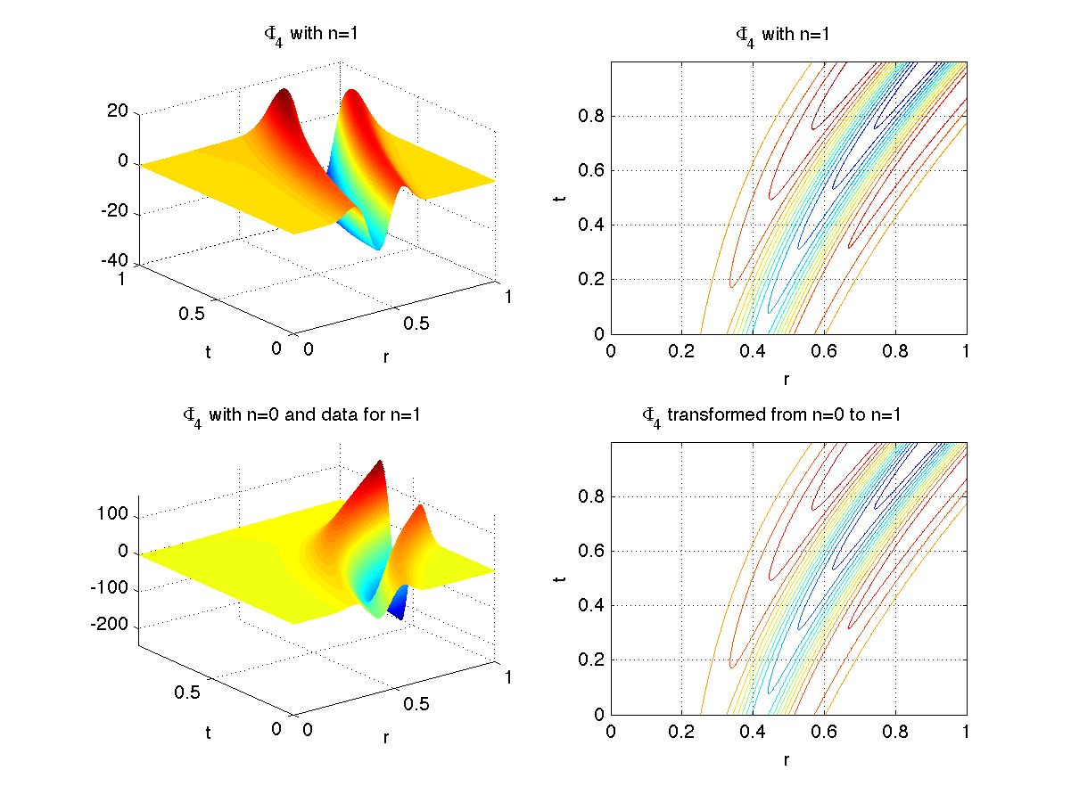
Figure 3: Comparison between the two representations. For detailed explanation see text.

In Fig. 3 we present the results of these operations. The surface plot in the upper left shows the component $\phi_{4}$ evolved with the diagonal representation $n=1$, while the plot on the lower left shows $\phi_{4}$ obtained in the horizontal representation using the same data as for the case $n=1$ but rescaled according to (15). The contour plots on the right show the obtained solutions. Above is the solution directly obtained in the diagonal representation while below is the solution obtained after rescaling back from the horizontal representation. The contour plots agree visually. Note, that the $t$ coordinates in the two surface plots are not the same. They refer to $t_{0}$ in the lower plot and to $t_{1}$ in the other.

In the horizontal representation we come arbitrarily close to $t=1$. Hence, we can ‘almost’ compute the entire space-time (at least in this simple set-up). In this sense the horizontal representation is much more efficient than the diagonal one. In Fig. 4

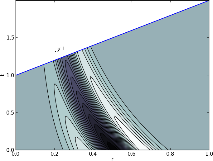
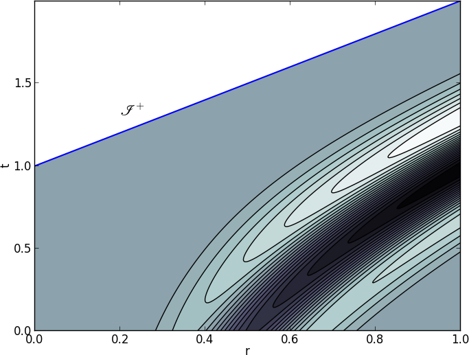
Figure 4: Contour plots of $\phi_{0}$ (left) and $\phi_{4}$ (right) computed with $n=0$ but rescaled to the diagonal representation.

we show the contour plots of the rescaled solution in the diagonal representation. Clearly, it extends way over the $t=1$ time-slice reaching $\mathscr{I}^{+}$ to within the graphical resolution.

5 Reaching null-infinity

Since the horizontal representation allows us to almost reach null-infinity one may wonder whether it might be possible to extend the computation to $\mathscr{I}^{+}$ from the last time-level at $t=\bar{t}$, say? To answer this question we refer back to Fig. 1 where we showed the space-time in the horizontal representation together with the two families of characteristics. The ‘outgoing’ characteristics (those intersecting $\mathscr{I}^{+}$) are well-behaved while the other family asymptotes to $I\cup\mathscr{I}^{+}$ in a non-uniform way. Referring to Eq. (7) we see that all components except for $\phi_{4}$ propagate along the well-behaved characteristics. This suggests that we use those four propagation equations to estimate the values of $\phi_{0}$, $\phi_{1}$, $\phi_{2}$, $\phi_{3}$ on $\mathscr{I}^{+}$. Since we cannot use any values of $\phi_{4}$ beyond $t=\bar{t}$ we are forced to use an Euler step to get to $t=1$.

As for $\phi_{4}$ we observe that its propagation equation reduces to an intrinsic equation on $\mathscr{I}^{+}$, which we could integrate if we had initial conditions for $\phi_{4}$ at $r=0$, once we know the values of the other components on $\mathscr{I}^{+}$. The equation for $\phi_{4}$ on $\mathscr{I}^{+}$ reduces to

$$r\partial_{r}\phi_{4}-2\phi_{4}=\alpha_{2}\phi_{3}.$$ (16)

This equation is singular at $r=0$ and the requirement that $\phi_{4}$ and its derivative be bounded forces the initial condition

$$\phi_{4}(1,0)=-\frac{\alpha_{2}}{2}\phi_{3}(1,0).$$

So we see that we can perform the last step to $\mathscr{I}^{+}$, albeit only with a first order method.

We tested this approach by evolving compactly supported initial data obtained by explicitly solving the constraints (the same ones as in Sec. 4). The error at $t=1$ was estimated by comparing the values produced in some simulation to the values produced in the highest resolution simulation with $6400$ grid points. The $L_{2}$ measure of the error is presented in Table 2. Since the $\phi_{0}$ and $\phi_{4}$ components mark the extreme cases, we do not present the error convergence rates for $\phi_{1},\phi_{2},\phi_{3}$. Their convergence rates are comparable to $\phi_{0}$.

	$\phi_{0}$		$\phi_{4}$
Grid Points	$\log_{2}(||\Delta||_{2})$	Rate	$\log_{2}(||\Delta||_{2})$	Rate
200	-7.99		0.082
400	-11.48	3.49	-0.44	0.52
800	-14.98	3.49	-1.02	0.57
1600	-18.48	3.50	-1.73	0.71
3200	-22.07	3.58	-2.81	1.08

Table 2: Absolute error $\Delta$ compared to a 6400 grid point simulation using the $L^{2}$ norm and convergence rates at time $t=1$ for $\phi_{0},\phi_{4}$ for compactly supported data in the $n=0$ space-time.

Remarkably, the convergence rate for $\phi_{0}$ is close to $4^{\text{th}}$ order, while for $\phi_{0}$ we get the expected first order convergence. The accuracy in the radiation component is roughly $10^{-7}$ while for $\phi_{4}$ it is not good, only $\approx 10\%$. This low accuracy is due to the singular behavior of the propagation equation (16) for $\phi_{4}$ at $r=0$, which we might not have taken care of appropriately. There is still room for improvement because we could use the intrinsic transport equations (see Beyer:2012ie ; Friedrich:2003hp ) along the cylinder—mentioned in the introduction—to drag along as many derivatives of $\phi_{4}$ as we please. These could be used to construct a Taylor approximation for $\phi_{4}$ near $r=0$ to get the integration process started more smoothly.

6 Conclusion

In this paper we have presented a study of the spin-2 equation in the neighborhood of spatial infinity in Minkowski space-time. Since the perturbations of the Weyl curvature on flat space obey this equation we can interpret this system as a model for small amplitude gravitational waves. We used this model to study the asymptotic properties of the fields —and, hence, to some extent also of the perturbed space-time—close to spatial infinity. This region is still not completely understood and we hope that our work will ultimately contribute to the complete understanding of this issue.

We have shown here that it is possible to generate a complete evolution from initial data on an asymptotically Euclidean hyper-surface to the asymptotic regime including null-infinity even though the equations show a certain degeneracy at the cylinder which represents spatial infinity in Friedrich’s conformal Gauß gauge. Using the horizontal representation as described in Sects. 4 and 5 we can get the radiation field $\phi_{0}$ quite accurately on $\mathscr{I}^{+}$. The drop in convergence for the component $\phi_{4}$ is akin to the loss of smoothness of null-infinity in the first result on the global stability of Minkowski space by Christodoulou and Klainerman Christodoulou:1993vm . This was caused by the loss of peeling in the corresponding component of the Weyl tensor.

Of course, we deal here with a highly simplified system and the fact that we can make things work here does not immediately imply that it will also work in the physically relevant 3D cases. However, this toy system does provide valuable insights into the possibilities of and the restrictions imposed by the structure of spatial infinity. We should point out that the structure of the fully non-linear general conformal field equations is very similar to the linear spin-2 system. This is essentially due to the fact that the spin-2 system results from the Bianchi equations obeyed by the rescaled Weyl spinor.

Our next steps will be the removal of the artificial boundary at $r=1$. This will allow us to perform an entirely global evolution of the mode decomposed spin-2 field. The challenge here is to get the centre under control because due to the spherical symmetry this will be a singular point for the equations. Then, we intend to remove the mode decomposition and look at the linearized system in three spatial dimensions.

- (1) Beyer, F., Doulis, G., Frauendiener, J.: Numerical space-times near space-like and null infinity. The spin-2 system on Minkowski space. Classical and Quantum Gravity 29(24), 245,013 (2012)
- (2) Bizoń, P., Rostworowski, A.: On weakly turbulent instability of anti-de Sitter space. Phys. Rev. Lett. 107 (2011)
- (3) Carpenter, M.H., Gottlieb, D., Abarbanel, S.: Time-stable boundary conditions for finite-difference schemes solving hyperbolic systems: methodology and application to high-order compact schemes. J. Comp. Phys. 111(2), 220–236 (1994)
- (4) Carpenter, M.H., Nordström, J., Gottlieb, D.: A stable and conservative interface treatment of arbitrary spatial accuracy. J. Comp. Phys. 148(2), 341–365 (1999)
- (5) Christodoulou, D., Klainerman, S.: The global nonlinear stability of the Minkowski space, vol. 41. Princeton University Press, Princeton (1993)
- (6) Diener, P., Dorband, E., Schnetter, E., Tiglio, M.: Optimized high-order derivative and dissipation operators satisfying summation by parts, and applications in three-dimensional multi-block evolutions. J Sci Comput 32(1), 109–145 (2007)
- (7) Frauendiener, J.: Numerical treatment of the hyperboloidal initial value problem for the vacuum Einstein equations. II. The evolution equations. Phys Rev D 58(6), 064,003 (1998)
- (8) Frauendiener, J.: Conformal infinity. Living Rev. Relativity 7, 2004–1, 82 pp. (electronic) (2004)
- (9) Friedrich, H.: Einstein equations and conformal structure: Existence of anti-de Sitter-type space-times. J. Geom. Phys. 17, 125–184 (1995)
- (10) Friedrich, H.: Gravitational fields near space-like and null infinity. J. Geom. Phys. 24, 83–163 (1998)
- (11) Friedrich, H.: Spin-2 fields on Minkowski space near spacelike and null infinity. Classical and Quantum Gravity 20(1), 101 (2003)
- (12) Friedrich, H.: Static Vacuum Solutions from Convergent Null Data Expansions at Space-Like Infinity. Annales de l’IHP A (2007)
- (13) Friedrich, H.: Conformal classes of asymptotically flat, static vacuum data. Classical and Quantum Gravity 25(6), 065,012 (2008)
- (14) Friedrich, H.: One-parameter families of conformally related asymptotically flat, static vacuum data. Classical and Quantum Gravity (2008)
- (15) Friedrich, H.: Conformal structures of static vacuum data. arXiv gr-qc (2012)
- (16) Friedrich, H., Schmidt, B.G.: Conformal Geodesics in General Relativity. Proc. Roy. Soc. A (1987)
- (17) Goldberg, J.N., Macfarlane, A., Newman, E.T.: Spin-s Spherical Harmonics and Eth. J Math Phys (1967)
- (18) Gustafsson, B., Kreiss, H.O., Oliger, S.: Time-dependent problems and difference methods. A Wiley-Interscience Publication (1995)
- (19) Lehner, L., Reula, O., Tiglio, M.: Multi-block simulations in general relativity: high-order discretizations, numerical stability and applications. Classical and Quantum Gravity 22(24), 5283 (2005)
- (20) Newman, E.T., Penrose, R.: New conservation laws for zero rest-mass fields in asymptotically flat space-time. Proc. Roy. Soc. A 305(1482), 175–204 (1968)
- (21) Penrose, R.: Zero rest-mass fields including gravitation: asymptotic behaviour. Proc. Roy. Soc. London A 284, 159–203 (1965)
- (22) Penrose, R., Rindler, W.: Spinors and Spacetime: Two-spinor calculus and relativistic fields, vol. 1. Cambridge University Press, Cambridge (1984)
- (23) Schnetter, E., Diener, P., Dorband, E.N., Tiglio, M.: A multi-block infrastructure for three-dimensional time-dependent numerical relativity. Classical and Quantum Gravity 23(16), S553–S578 (2006)
- (24) Strand, B.: Summation by Parts for Finite Difference Approximations for d/dx. J. Comp. Phys. 110(1), 47–67 (1994)