Synthesis of Multivalued Quantum Logic Circuits by Elementary Gates

Abstract

We propose the generalized controlled $X$ (GCX) gate as the two-qudit elementary gate, and based on Cartan decomposition, we also give the one-qudit elementary gates. Then we discuss the physical implementation of these elementary gates and show that it is feasible with current technology. With these elementary gates many important qudit quantum gates can be synthesized conveniently. We provide efficient methods for the synthesis of various kinds of controlled qudit gates and greatly simplify the synthesis of existing generic multi-valued quantum circuits. Moreover, we generalize the quantum Shannon decomposition (QSD), the most powerful technique for the synthesis of generic qubit circuits, to the qudit case. A comparison of ququart ($d=4$) circuits and qubit circuits reveals that using ququart circuits may have an advantage over the qubit circuits in the synthesis of quantum circuits.

I Introduction

Using multivalued quantum systems (qudits) instead of qubits has a number of potential advantages. As a specific name, three-level quantum systems are called qutrits, and four-level systems are also called ququarts. There have been many proposals to use qudits to implement quantum computing 1 ; 2 ; 3 ; 4 ; 5 ; 6 . Now there is an increasing interest in this area, and some experimental works on qudit systems have been developed in recent years 7 ; 8 ; 9 .

Many works have been done in multivalued quantum logic synthesis. Brylinski and Brylinski 10 and Bremner et al. 11 concluded that any two-qudit gate that creates entanglement without ancillas can act as a universal gate for quantum computation, when assisted by arbitrary one-qudit gates. Brennen et al. proposed use of the controlled increment (CINC) gate as a two-qudit elementary gate, investigated the synthesis of general qudit circuits based on spectral decomposition, and the “Triangle” algorithm 4 ; 5 , and obtained asymptotically optimal results, but for the synthesis of specific qudit gates, using this gate is inconvenient and the relevant work is rarely seen. There are other proposals, such as the GXOR 3 , SUM 6 , etc., but no practice circuits are given. The synthesis of binary quantum circuits has been extensively investigated by many authors 12 ; 13 ; 14 ; 15 ; 16 ; 17 ; 18 ; 19 ; 20 ; 21 ; 22 , and it is rather mature now. In the previous work for qudit circuits the methods in qubit circuits are seldom used. Since there are technical difficulties 23 with the tensor product structure of qudits, whether these methods are useful for qudits has been an open question. Moreover, there is no unified measure for the complexity of qubit and various qudit circuits yet, which makes it inconvenient to compare them.

In this article we focus on the synthesis of multivalued quantum logic circuits. With the elementary gates proposed here we can synthesize many specific qudit quantum gates conveniently, greatly simplify the synthesis of existing generic multi-valued quantum circuits, generalize the quantum Shannon decomposition (QSD) 20 , the most powerful technique for the synthesis of generic qubit circuits, to the qudit case and get many best known results. Moreover, the defects mentioned above are all overcome.

The article is organized as follows. In Sec. II we propose the general controlled $X$ (GCX) gate as a two-qudit elementary gate, and based on Cartan decomposition 24 we also give a set of one-qudit elementary gates. They can be used as a unified measure of complexity for various quantum logic circuits. In Sec. III we investigate the physical implementation of these gates and show that it is feasible with current technology. With these gates we investigate the synthesis of some important multivalued quantum gates and the synthesis of various controlled qudit gates in Sec. IV. We generalize the QSD to qudit case in Sec. V, revealing that using ququart circuits may have an advantage over the qubit circuits in the synthesis of quantum circuits. Finally, a brief conclusion is given in Sec. VI. The Cartan decomposition used in Sec. II is given in Appendix A.

II Elementary gates

There are $d(d-1)/2$ single-qudit $X^{(ij)}$ gates which act on the two-dimensional subspace $\mathscr{H}_{ij}$ of $d$-dimensional Hilbert space, where $X^{(ij)}=|i\rangle\langle j|+|j\rangle\langle i|+\sum_{k\neq i,j}|k\rangle\langle k|$. The GCX gate is the two-qudit gate which implements the $X^{(ij)}$ operation on the target qudit iff the control qudit is in the state $|m\rangle$, $(m\in\{0,1,\ldots,d-1\})$. The circuit representation for the GCX gate is shown in Fig. 1, in which the line with a circle represents the control qudit while that with a square the target qudit. There are $d^{2}(d-1)/2$ different forms of the gate and they can be easily transferred to one another as shown in Fig. 2.

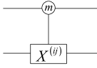
Figure 1: Generalized controlled-$X$ gate.

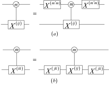
Figure 2: Transformation among different GCX gates: (a) transformation of control mode. (b) transformation of target operations.

The CINC gate is a controlled one-qudit gate which implements the INC operation on the target qudit iff the control qudit is in the states $|m\rangle$, where INC$|j\rangle=|j+1,mod\;d\rangle$. The INC operation can be decomposed into $d-1$ $X$ operations, so the CINC gate can be synthesized by $d-1$ GCX gates. The GCX gate is an elementary counterpart of the binary CNOT gate, so we propose the GCX gate as the two-qudit elementary gate for multivalued quantum computing. It can be used as a unified measure for the complexity of various quantum circuits.

Suppose $M$ is the matrix of a one-qutrit gate. Take a kind of AIII type Cartan decomposition 23 of the $\mathrm{U}(3)$ group, which can be expressed as

$$M=e^{i\varphi}M_{1}^{(jk)}M^{(j^{\prime}k^{\prime})}M_{2}^{(jk)}.$$ (1)

Here $M^{(jk)}$ is a special unitary transformation in two-dimensional subspace $\mathscr{H}_{jk}$, and it can be factored further by the Euler decomposition. The Euler decomposition usually has two modes: $ZYZ$ decomposition and $XYX$ decomposition. So the set of one-qutrit elementary gates has two pairs of basic gates, $R_{y}^{(jk)}$, $R_{z}^{(jk)}$, $R_{y}^{(j^{\prime}k^{\prime})}$, $R_{z}^{(j^{\prime}k^{\prime})}$ or $R_{x}^{(jk)}$, $R_{y}^{(jk)}$, $R_{x}^{(j^{\prime}k^{\prime})}$, $R_{y}^{(j^{\prime}k^{\prime})}$. Here $R_{\alpha}^{(jk)}(\theta)=\exp(-i\theta\sigma_{\alpha}^{(jk)}/2)$, for $0\leq j<k\leq 2$, $\alpha\in\{x,y,z\}$, and $\sigma_{x}^{(jk)}=|j\rangle\langle k|+|k\rangle\langle j|$, $\sigma_{y}^{(jk)}=-i|j\rangle\langle k|+i|k\rangle\langle j|$, $\sigma_{z}^{(jk)}=|j\rangle\langle j|-|k\rangle\langle k|$.

Using successive AIII-type Cartan decompositions of the $\mathrm{U}(d)$ group, a generic one-qudit gate can be decomposed to a series of $M^{(jk)}$, which involves at least $d-1$ kinds of $M^{(jk)}$ that act on different 2D subspaces. To implement a qudit gate requires $d-1$ driving fields, and $M^{(jk)}$s essentially are single-qubit gates. So the set of one-qudit elementary gates has $d-1$ pairs of $R_{\alpha}^{(jk)}$ gates acting on $d-1$ different 2D subspaces. The choice of $d-1$ pairs of basic gates is not unique. They are universal if only the corresponding driving fields can connect the $d$ levels of the qudit together.

III Physical implementation

In the last decade, there has been tremendous progress in the experimental development of qubit quantum computing, and the problem of constructing a CNOT gate has been addressed from various perspectives and for different physical systems 25 ; 26 ; 27 ; 28 ; 29 ; 30 ; 31 ; 32 ; 33 ; 34 ; 35 ; 36 . The GCX gate is essentially binary, so it can be implemented with existing technique.

Figure 3: V-type three level quantum system.

Assume we have a V-type three-level quantum system shown in Fig. 3, which constitutes a qutrit and the two levels of the system $|0\rangle$ and $|1\rangle$ forms a qubit. Two laser beams $\Omega_{1}$ and $\Omega_{2}$ are applied to the ion to manipulate $|0\rangle\leftrightarrow|1\rangle$ and $|0\rangle\leftrightarrow|2\rangle$ transition, respectively. If a two-qubit CNOT gate is realized in such systems, one GCX gate is naturally obtained, and the eight other GCX gates formed can be obtained by the transformation shown in Fig. 2. The single-qutrit gates are implemented by Rabi oscillations between the qutrit levels. Applying the laser pulses in $\Omega_{1}$ and $\Omega_{2}$ and choosing suitable phases, this allows us to perform $R_{x}^{(01)}$, $R_{y}^{(01)}$ and $R_{x}^{(02)}$, $R_{y}^{(02)}$ gates, respectively 37 ; 38 . So a set of one-qutrit elementary gates is obtained, and any one-qutrit gate can be implemented according to Eq. (4). There are two other types of quantum system: the $\Lambda$ type and cascade type. We can use $R_{x}^{(01)}$, $R_{y}^{(01)}$, $R_{x}^{(12)}$, $R_{y}^{(12)}$ or $R_{y}^{(02)}$, $R_{z}^{(02)}$, $R_{y}^{(12)}$, $R_{z}^{(12)}$ as one-qutrit elementary gates to meet the requirement of manipulating quantum states in these types of quantum systems. The method can be naturally generalized to the generic qudit case.

It is not too difficult to find such a quantum system. Early in 2003, the Innsbruck group implemented the complete Cirac-Zoller protocol 25 of the CONT gate with two calcium ions ($\mathrm{Ca^{+}}$) in a trap 27 . The original qubit information is encoded in the ground-state $S_{1/2}$ and metastable $D_{5/2}$ state. The $D_{5/2}$ state has a lifetime $\tau\backsimeq 1.16$ s. There is another metastable $D_{3/2}$ state in $\mathrm{Ca^{+}}$. Its lifetime is about the same as that of the $D_{5/2}$ state. The three levels of $\mathrm{Ca^{+}}$, one ground state and two metastable states, may constitute a qutrit candidate. The CNOT gate was implemented by Schmidt-Kaler et al. 27 and forms naturally a TCX gate. Two laser pulses are used to manipulate the $S_{1/2}\leftrightarrow D_{5/2}$ quadruple transition near 729 nm and the $S_{1/2}\leftrightarrow D_{3/2}$ transition near 732 nm, respectively. Rabi oscillations between these levels can implement the one-qutrit elementary gates $R_{x}^{(01)}$, $R_{y}^{(01)}$ and $R_{x}^{(02)}$, $R_{y}^{(02)}$.

The superconducting quantum information processing devices are typically operated as qubit by restricting them to the two lowest energy eigenstates. By relaxing this restriction, we can operate it as a qutrit or qudit. The experimental demonstrations of the tomography of a transmon-type superconducting qutrit have been reported in 9 , and the emulation of a quantum spin greater than $1/2$ has been implemented in a superconducting phase qudit 8 . This means that to prepare a one-qutrit state or one-qudit state and a read out on these systems has been implemented, so the one-qutrit gates or one-qudit gates can also be implemented on the systems. Construction of a robust CNOT gate on superconducting qubits has been extensively investigated 34 ; 35 ; 36 , which means that the condition to implement multivalued quantum computing has come to maturity on these superconducting devices.

IV Synthesis of multi-valued quantum logic gates

IV.1 Synthesis of some important multi-valued quantum gates

By using GCX gates, some important qudit gates can be synthesized conveniently. The reason is that the $X^{(i,\,i+1)}$’s operations are the generators of the permutation group $S_{d}$, while INC, etc. operations are not. The multivalued SWAP gate interchanges the states of two qudits acted on by the gate. The ternary SWAP gate can be decomposed into three binary SWAP gates, that is

$$W=W^{(01)}\cdot W^{(02)}\cdot W^{(12)}.$$ (2)

Here $W^{(ij)}=|ij\rangle\langle ji|+|ji\rangle\langle ij|+\sum_{kl\neq ij,ji}|kl\rangle\langle kl|$, and it can be synthesized by three GCX gates. So the ternary SWAP gate is synthesized by nine GCX gates. For the generic qudit case, the multivalued SWAP gate can be decomposed into $d(d-1)/2$ binary SWAP gates, each of them needing three GCX gates. The multivalued root SWAP gate can also be decomposed into $d(d-1)/2$ binary root SWAP gates.

We denote two inputs of a $d$-dimensional two-qudit as $A$ and $B$, respectively. The SUM gate is a two-qudit gate in which an output remains $A$ unchanged, and another output is the sum of $A$ and $B$ modulo $d$ denoted $A\oplus B$. The GXOR gate is similar to the SUM gate. The difference is that the output is the difference of $A$ and $B$ modulo $d$. The synthesis of the ternary SUM gate and ternary GXOR gate base on the GCX gates is shown in Fig. 4 and Fig. 5, respectively.

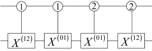
Figure 4: Synthesis of ternary SUM gate.

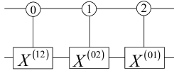
Figure 5: Synthesis of ternary GXOR gate.

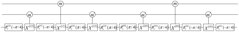
Figure 6: Synthesis of the ternary $\wedge_{2}$(INC) gate.

The twofold generalized controlled $X$ gate [$\wedge_{2}(X)$] is a three-qudit gate in which two control qudits are unaffected by the action of the gate, and the target qudit is acted on by the $X^{(ij)}$ operation iff the two control qudits are in the states $|m\rangle$, $|m^{\prime}\rangle$ respectively. It is essentially a Toffoli gate 37 , which can be synthesized with six GCX gates and ten single-qudit gates acting on a 2D subspace. In some cases, we can use the psuedo-$\wedge_{2}(X)$ gate $\left(p\wedge_{2}\left(X\right)\right)$ instead of the $\wedge_{2}(X)$ gate. The $p\wedge_{2}(X)$ gate is also a three-qudit gate that two control qudits are unaffected by the action of the gate, the target qudit is acted by the $X^{(ij)}$ operation iff the two control qudits are in the states $|m\rangle$, $|m^{\prime}\rangle$ respectively and by the $Z^{(ij)}$ or $Z^{(ji)}$ operation iff the first control qudit is in the state $|m\rangle$, the second control qudit is not in the state $|m^{\prime}\rangle$. It is synthesized by three GCX gates and two $R_{\alpha}^{(ij)}(\pi/4)$ and two $R_{\alpha}^{(ij)}(-\pi/4)$ gates (see Appendix B). The two-fold controlled INC gate [$\wedge_{2}$(INC)] is that the two qudits remain no change, the qudit is acted by the INC operation iff two control qudits are in the control states $|m\rangle$, $|m^{\prime}\rangle$ respectively. The ternary $\wedge_{2}$(INC) gate consists of two $p\wedge_{2}(X)$ gates, and the synthesis is shown in Fig. 6, which requires six GCX gates and eight $R_{y}^{(ij)}(\theta)$ gates. In $d$-valued qudit case, the synthesis of $\wedge_{2}$(INC) gate requires $3(d-1)$ GCX gates for $d$ is odd, and $3d$ GCX gates for $d$ is even. It is much simpler than that in 5 . That needs $(d+2)d$ CINC gates and $(d+1)d$ CINC^-1 gates, which is equivalent to $(2d+3)d(d-1)$ GCX gates.

IV.2 Synthesis of various controlled qudit gates

A controlled one-qudit gate [$\wedge_{1}(U)$] is a two-qudit gate in that iff the control qudit is set to the state $|m\rangle$ then a unitary operation $U$ is applied to the target qudit. From the diagonal decomposition $U=VDV^{\dagger}$, we can get a synthesis of a controlled $U$ gate which involves a pair of one-qudit gates and a controlled diagonal [$\wedge_{1}(\bigtriangleup)$] gate as shown in Fig.7. Here $V$ is unitary, and $D$ is diagonal and has the form

$$D = e^{\varphi}diag\{e^{-i(\alpha_{1}+\alpha_{2}+\ldots+\alpha_{d-1})},e^{i\alpha_{1}},e^{i\alpha_{2}},\ldots,e^{i\alpha_{d-1}}\}$$ (3)

$$= e^{\varphi}R_{z}^{(01)}(\alpha_{1})R_{z}^{(02)}(\alpha_{2})\ldots R_{z}^{(0(d-1))}(\alpha_{d-1}).$$

The $\wedge_{1}(\bigtriangleup)$ gate can be synthesized by a phase qudit and $d-1$ controlled $R_{z}^{(ij)}$ gates, each of them needing two GCX gates. Hence the generic $\wedge_{1}(U)$ gate can be synthesized by $2(d-1)$ GCX gates in the worst case. In qutrit case the synthesis of a $\wedge_{1}(\bigtriangleup)$ gate is shown in Fig. 8, where $S_{m}=\sum_{j}(1+\delta_{jm}(e^{i\varphi}-1)|j\rangle\langle j|$ is a phase qutrit gate.

The $k$-fold controlled one-qudit gate [$\wedge_{k}(U)$] has $k$ control qudits and a target qudit. Similar to the synthesis of the $\wedge_{1}(U)$ gate, a $\wedge_{k}(U)$ gate is composed of a pair of one-qudit gates and a $k$-fold controlled one-qudit diagonal one-qudit gate $[\wedge_{k}(\bigtriangleup)]$. The $\wedge_{k}(\bigtriangleup)$ gate can be synthesized by a $(k-1)$-fold controlled phase qudit and $d-1$ $\wedge_{k}(R_{z})$ gates, and each $\wedge_{k}(R_{z})$ needs a pair of $\wedge_{k}(X)$ gates. To simplify the synthesis of $\wedge_{k}(U)$ gates, we introduce the pseudo-$\wedge_{k}(X)$ [$p\wedge_{k}(X)$] gates. The $p\wedge_{k}(X)$ gate has two sets of control qudits. Its target qudit is acted by the $X^{(ij)}$ operation iff the two sets of control qudits are in the control states $|m_{1},m_{2},\cdots,m_{k_{1}}\rangle$ and $|m_{1}^{\prime},m_{2}^{\prime},\cdots,m_{k_{2}}^{\prime}\rangle$, respectively, and by the $Z^{(ij)}$ operation iff the first set of control qudits is in the control states and the second set of control qudits is not in the control states, where $k_{1}+k_{2}=k$. Now we present a scheme for implementing $p\wedge_{k}(X)$ gates and a scheme for implementing $\wedge_{k}(X)$ gates, shown in Fig. 9 and 10, respectively. Since the $\wedge_{k}(X)$ gates appear in the $\wedge_{k}(R_{z})$ gate in a pair and the $R_{z}$ gates are diagonal, they can be replaced by $p\wedge_{k}(X)$ gates. The $k$-fold controlled unimodular one-qudit gate can be synthesized by $2p_{k}(d-1)$ GCX gates. Here $p_{k}$ denotes the numbers of GCX gates in a $p\wedge_{k}(X)$ gate, and it can be obtained by its recursive implementing process. The $(k-1)$-fold controlled phase gate can be further decomposed into a $(k-1)$-fold controlled unimodular diagonal gate and a $(k-2)$-fold controlled phase gate. By successive decomposition we can get that the synthesis of a $k$-fold controlled general one-qudit gate requires $2(1+\sum_{s=2}^{k}p_{s})(d-1)\leq(1+\delta_{n2})k^{3}(d-1)$ GCX gates. The estimate $2(1+\sum_{s=2}^{k}p_{s})\leq(1+\delta_{n2})k^{3}$ comes from practice data.

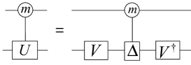
Figure 7: Synthesis of a controlled $U$ gate.

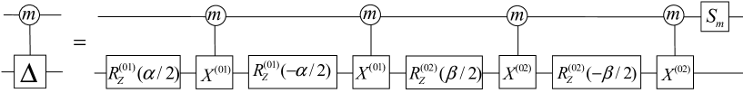
Figure 8: Synthesis of a controlled diagonal qutrit gate.

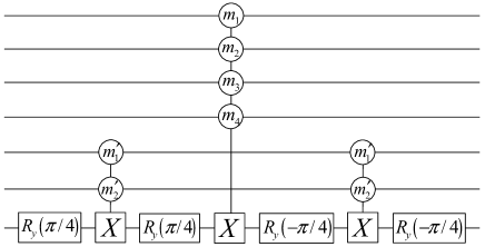
Figure 9: A circuit implementing a $p\wedge_{k}(X)$ gate.

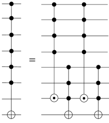
Figure 10: A circuit implementing $\wedge_{k}(X)$ gate. For brief, the symbols in the qubit circuit are used and the $\odot$ denotes the pseudo-$X$ operation.

With efficient synthesis of $\wedge_{1}(U)$ and $\wedge_{k}(U)$ gates we can greatly simplify the synthesis of existing multiqudit circuits. Based on the spectral decomposition, for the circuit without ancillas, the GCX count of generic $n$-qudit circuits is

$$C_{s} = 2d^{n}[(d^{n}-1)-n(d-1)]+2(1+\sum_{s=2}^{n-1}p_{s})d^{n}(d-1)$$ (4)

$$\leq 2d^{n}[(d^{n}-1)-n(d-1)]$$

$$+ (1+\delta_{n2})(n-1)^{3}d^{n}(d-1),$$

whereas the CINC count using the spectral decomposition given in 5 is

$$\ell_{s}\leq 2d^{n+1}[(d^{n}-1)/(d-1)-n]+(n+1)^{2+\log_{2}d}d^{n+4}.$$ (5)

V Quantum shannon decomposition

A $n$-qudit gate corresponds to a $d^{n}\times d^{n}$ unitary matrix. Using Cosine-sine decomposition (CSD) 14 ; 39 we decompose it to $d^{n-1}\times d^{n-1}$ block diagonal matrices and cosine-sine matrices. The block diagonal matrix is a uniformly controlled multi-qudit gate, which can be reduced to a $(n-1)$-qudit gate and $d-1$ copies of controlled ($n-1$)-qudit $[\wedge_{1}(U(d^{n-1}))]$ gates. It can be further reduced to $d$ copies of $(n-1)$-qudit gates and $d-1$ copies of ($n-1$)-qudit diagonal $(\wedge_{1}(\Delta_{n-1}))$ gates as shown in Fig. 11. Taking $d=2$, the related decomposition of a block diagonal matrix is

$$\left(\begin{array}[]{cc}U_{1}&\\ &U_{2}\\ \end{array}\right)=\left(\begin{array}[]{cc}V_{1}&\\ &V_{1}\\ \end{array}\right)\left(\begin{array}[]{cc}I&\\ &\Delta_{n-1}\\ \end{array}\right)\left(\begin{array}[]{cc}V_{2}&\\ &V_{2}\\ \end{array}\right).$$ (14)

It is equivalent to the decomposition

$$\left(\begin{array}[]{cc}U_{1}&\\ &U_{2}\\ \end{array}\right)=\left(\begin{array}[]{cc}W&\\ &W\\ \end{array}\right)\left(\begin{array}[]{cc}D&\\ &D^{{\dagger}}\\ \end{array}\right)\left(\begin{array}[]{cc}V&\\ &V\\ \end{array}\right),$$ (23)

where $W=V_{1}\Delta_{n-1}^{1/2}$, $D=\Delta_{n-1}^{-1/2}$ and $V=V_{2}$. It is just the decomposition of block diagonal matrices in QSD. So the decomposition given here for qudit circuit can be considered as a generalized QSD.

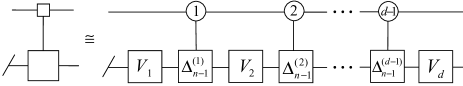
Figure 11: Decomposition of a uniformly controlled multiqudit gate. Here the small square ($\Box$) denotes uniform control and the slash (/) represents multiple qudits on the line.

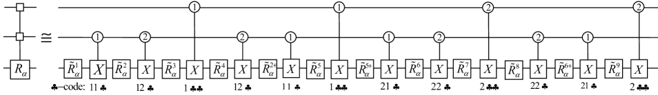
Figure 12: Quantum circuit implementing ternary uniformly two-fold controlled $R_{\alpha}^{(ij)}(\alpha\in y,z)$ rotation. Here we use $\tilde{R}_{\alpha}^{k}=R_{\alpha}^{(ij)}(\theta_{k})$, and the $\clubsuit$ codes without zero entry are used to define the position of the control nodes of GCX gates.

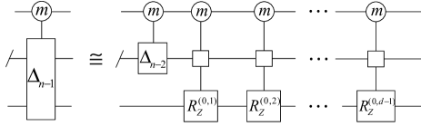
Figure 13: Quantum circuit implementing a $\wedge_{1}(\bigtriangleup_{n-1})$ gate

Here we give a very efficient synthesis of the multivalued uniformly multifold controlled $R_{\alpha}^{(ij)}(\alpha\in y,z)$ rotation. The method parallels the techniques in 14 ; 40 for the qubit case. For $d=3$ and $n=3$, its synthesis is shown in Fig. 12, and in the generic case, it needs $2d^{n-2}(d-1)$ GCX gates (see Appendix C). The circuit can be conveniently obtained by the $\clubsuit$ sequence 4 . To divide the elements of a $\wedge_{1}(\bigtriangleup_{n-1})$ gate into $d^{n-2}$ groups and factor out a phase for each group to make it unimodular, we get a circuit of the gate as shown in Fig.13. It can be further inferred that it needs $2(d^{n-1}-1)$ GCX gates for the synthesis of a $\wedge_{1}(\bigtriangleup_{n-1})$ gate.

Table 1: Exact GCX gate count for the synthesis of qudit quantum circuits obtained using the QSD decomposition. Here $\divideontimes$ means this count is better than that using the spectral algorithm obtained by Eq.(4).

	$d=3$	$d=4$	$d=5$	$d=6$	$d=7$	$d=8$
2	$\divideontimes$44	$\divideontimes$108	$\divideontimes$272	$\divideontimes$510	$\divideontimes$828	$\divideontimes$1176
3	$\divideontimes$692	$\divideontimes$2232	$\divideontimes$10256	$\divideontimes$25860	$\divideontimes$52740	$\divideontimes$85456
4	$\divideontimes$6860	$\divideontimes$37800	$\divideontimes$336144	$\divideontimes$1158720	$\divideontimes$2965788	$\divideontimes$5551504
5	$\divideontimes$83924	$\divideontimes$613248	$\divideontimes$10796560	$\divideontimes$51109320	$\divideontimes$166400964	$\divideontimes$355955600
6	$\divideontimes$1011932	$\divideontimes$7392768	$\divideontimes$345689872	$\divideontimes 2.25\times 10^{9}$	$\divideontimes 9.32\times 10^{9}$	$\divideontimes 2.28\times 10^{10}$
7	12157748	$\divideontimes$118419456	$\divideontimes 1.11\times 10^{10}$	$\divideontimes 9.90\times 10^{10}$	$\divideontimes 5.22\times 10^{11}$	$\divideontimes 1.46\times 10^{12}$
8	145936700	$\divideontimes 1.90\times 10^{9}$	$3.55\times 10^{11}$	$\divideontimes 4.36\times 10^{12}$	$\divideontimes 2.92\times 10^{13}$	$\divideontimes 9.34\times 10^{13}$

Table 2: A Comparison of gate counts of ququart circuits and qubit circuits 20 based on QSD. The index $l$ denotes the recursion bottoms, with which the results come out, at one-qubit or one-ququart gates ($l=1$), or two-qubit gates ($l=2$).

	1	2	3	4	n
$n$-ququart gate ($l=1$)	0	108	2232	37800	$(47/80)\times 4^{2n}-(11/4)\times 4^{n}+8/5$
$2n$-qubit gate ($l=1$)	6	168	2976	48768	$(3/4)\times 4^{2n}-(3/2)\times 4^{n}$
$2n$-qubit gate ($l=2$)	3	120	2208	36480	$(9/16)\times 4^{2n}-(3/2)\times 4^{n}$
$2n$-qubit gate ($l=2$, optimal)	3	100	1868	30927	$(23/48)\times 4^{2n}-(3/2)\times 4^{n}+4/3$

Taking $d=4$ as an example, using CSD, the matrix of an $n$-ququart circuit can be decomposed into four block diagonal matrices and three cosine-sine matrices. Each of the block diagonal matrices involves four ($n-1$)-ququart gates and three controlled diagonal ($n-1$)-ququart gates, and each of the cosine-sine matrices involves two uniformly ($n-1$)-fold controlled $R_{y}$ rotations. So a generic $n$-ququart circuit involves 16 ($n-1$)-ququart gates, 12 controlled diagonal ($n-1$)-ququart gates, and six uniformly ($n-1$)–fold controlled $R_{y}$ rotations. From these, we can calculate the GCX gate count based on QSD.

The exact GCX counts based on generalized QSD are tabulated in Table 1. When the number of qudits $n$ is small, it gives the simplest known quantum circuit, and when $d$ is a power of two, the circuits given here have the best known asymptotic features. The $n$-ququart ($d=4$) gate is needed asymptotically $O(47/80\times 4^{2n})$ GCX gates, whereas it needs asymptotically $O(2\times 4^{2n})$ GCX gates based on a spectral algorithm. Moreover, we compare ququart circuits with qubit circuits based on QSD in Table 2. Here the gate counts of a generic $n$-ququart circuit are obtained with recursion bottoms out at one-ququart gates ($l=1$); they are smaller than that of the corresponding $2n$-qubit circuit ($l=1)$. The counts can be improved further by finding more efficient synthesis of two-qudit gates and using some special optimal techniques. From this, the advantage of ququart over qubit in the synthesis of generic quantum circuits has been presented in the first time.

VI CONCLUSION

We propose the GCX gate as the twoqudit elementary gate of multivalued quantum circuits, and based on Cartan decomposition, the one-qudit elementary gates are also given. They are simple, efficient, and easy to implement. With these gates, various qudit circuits can be efficiently synthesized. Moreover, it can be used as a unified measure for the complexity of various quantum circuits. So the crucial issue of which gate is chosen as the elementary gate of qudit circuits is addressed. In spite of the difficulties with the tensor product structure of qudits, the methods used in qubit circuits still can play a very important role. The comparison of ququart circuits and qubit circuits based on QSD reveals that using ququart circuits may have an advantage over the qubit circuits in the synthesis of quantum circuits.

Multivalued quantum computing is a new and exciting research area. In the synthesis of multivalued quantum circuits there is still plenty of work to do. It will further reveal the advantage of qudit circuits over the conventional qubit circuits. Choosing a suitable quantum system, such as trapped ions, superconducting qudits, and quantum dots, to investigate the physical implementation of multivalued quantum logic gates and undertaking the experimental work is crucial for the development of multivalued quantum information science.

Appendix A CARTAN DECOMPOSITON

The Cartan decomposition of a Lie group depends on the decomposition of its Lie algebras 24 . Let $\mathfrak{g}$ be a semisimple Lie algebra and there is the decomposition

$$\mathfrak{g}=\mathfrak{l}\oplus\mathfrak{p},$$ (1)

where $\mathfrak{l}$ and $\mathfrak{p}$ satisfy the commutation relations

$$[\mathfrak{l},\mathfrak{l}]\subseteq\mathfrak{l},[\mathfrak{l},\mathfrak{p}]\subseteq\mathfrak{p},[\mathfrak{p},\mathfrak{p}]\subseteq\mathfrak{l},$$ (2)

where we said the decomposition is the Cartan decomposition of Lie algebra $\mathfrak{g}$. The $\mathfrak{l}$ is closed under the Lie bracket, so it is a Lie subalgebra of $\mathfrak{g}$, and $\mathfrak{p}=\mathfrak{l}^{\bot}$. A maximal Abelian subalgebra $\mathfrak{a}$ contained in $\mathfrak{p}$ is called a Cartan subalgebra. Then the element $M$ of Lie group $G$ can be decomposed as

$$M=K_{1}AK_{2},$$ (3)

where $G=e^{\mathfrak{g}}$, $K_{1},K_{2}\in e^{\mathfrak{l}}$, and $A\in e^{\mathfrak{a}}$.

For the qutrit case, we have eight independent ternary Pauli’s matrices: three $\sigma_{x}^{(ij)}$ matrices, three $\sigma_{y}^{(ij)}$ matrices, and two independent $\sigma_{z}^{(ij)}$ matrices in the three of them. Multiplying these eight Pauli’s matrices by $i$, we get the basis vectors of Lie algebra $\mathrm{su}(3)$ which we called the qusi–spin basis. Together with the $3\times 3$ identity matrix multiplied by $i$, they constitute the basis vectors of Lie algebra $\mathrm{u}(3)$. Take a kind of AIII-type Cartan decomposition 24 of $\mathrm{u}(3)$, that is

$$\mathrm{u}(3)=\mathrm{s}(\mathrm{u}(2)\oplus\mathrm{u}(1))\oplus\mathrm{s}(\mathrm{u}(2)\oplus\mathrm{u}(1))^{\bot}.$$ (4)

Lie subalgebra $\mathrm{s}(\mathrm{u}(2)\oplus\mathrm{u}(1))$ consists of subagebra $\mathrm{su}(2)$ and a complex basis $r=diag\{I_{2},-2\}=2\sigma_{z}^{(02)}-\sigma_{z}^{(01)}$. We choose

$$\mathrm{s}(\mathrm{u}(2)\oplus\mathrm{u}(1))=\text{span}\{i(\sigma_{x}^{(01)},\sigma_{y}^{(01)},\sigma_{z}^{(01)},r)\}$$ (5)

and its Cartan subalgebra

$$\mathfrak{a}=\text{span}\{i(I_{3},i\sigma_{y}^{(02)}\}.$$ (6)

So the one-qutrit matrix can be decomposed as

$$M = e^{i\alpha}\tilde{M}_{1}^{(01)}R_{z}^{(01)}(-\theta)R_{z}^{(02)}(2\theta)R_{y}^{(02)}(\beta)$$ (7)

$$R_{z}^{(02)}(2\theta^{\prime})R_{z}^{(01)}(-\theta^{\prime})\tilde{M}_{2}^{(01)}$$

$$= e^{i\alpha}M_{1}^{(01)}M^{(02)}M_{2}^{(01)}.$$

Lie subalgebra and Cartan subalgebra of the Cartan decomposition can be different, so the decomposition is not unique, and we can get the more generic Eq. (1) in Sec. II.

For the generic qudit case, we can also use the qusi–spin basis. There are $\frac{1}{2}d(d-1)$ $\sigma_{x}^{(ij)}$ matrices, $\frac{1}{2}d(d-1)$ $\sigma_{y}^{(ij)}$ matrices, and $d-1$ independent $\sigma_{z}^{(ij)}$ matrices for an $n$–dimensional Hilbert space. Multiplying these $d^{2}-1$ independent qusi-spin matrices by $i$, we gain the basis vectors of the Lie algebra $\mathrm{su}(d)$. Together with a $d\times d$ identity matrix multiplied by $i$, they constitute the basis vectors of Lie algebra $\mathrm{u}(d)$. We also take a kind of AIII-type Cartan decomposition for $\mathrm{u}(d)$, that is,

$$\mathrm{u}(d)=\mathrm{s}(\mathrm{u}(d-1)\oplus\mathrm{u}(1))+\mathrm{s}(\mathrm{u}(d-1)\oplus u(1))^{\perp}.$$ (8)

Lie algebra $\mathrm{s}(\mathrm{u}(d-1)\oplus\mathrm{u}(1))$ consists of subalgebra $\mathrm{su}(d-1)$ and a complex basis $r=diag\{I_{d-1},-(d-1)\}$. We choose its Cartan subalgebra

$$\mathfrak{\alpha}=span\{i(I_{d},\sigma_{y}^{(d-2,d-1)})\}.$$ (9)

So the arbitrary one–qudit matrix can be expressed as

$$M=e^{i\alpha}K_{1}R_{y}^{(d-2,d-1)}(\beta)K_{2},$$ (10)

where $K_{i}\in\mathrm{S}(\mathrm{U}(d-1)\oplus\mathrm{U}(1))$ group. The matrix $M$ can be re-expressed as

$$M = e^{i\mathfrak{\alpha}}\tilde{K^{\prime}_{1}}e^{i\theta r}R_{y}^{(d-2,d-1)}(\beta)e^{i\theta^{\prime}r}\tilde{K^{\prime}_{2}}$$ (11)

$$= e^{i\mathfrak{\alpha}}K^{\prime}_{1}M^{(d-2,d-1)}K^{\prime}_{2}.$$

where $\tilde{K^{\prime}_{i}},K^{\prime}_{i}\in\mathrm{SU}(d-1)\oplus 1$. That is because that $r$ can be expressed as a linear combination of $\sigma_{z}^{(jk)}$s, $r=\sigma_{z}^{(0,\,d-2)}+\cdots+\sigma_{z}^{(d-3,d-2)}+(d-1)\sigma_{z}^{(d-2,\,d-1)}$, so the $e^{i\theta r}$ is a product of a series of $R_{z}^{(jk)}$s. The $R_{y}^{(d-2,\,d-1)}$ combines with $R_{z}^{(d-2,\,d-1)}$ in $e^{i\theta r}$ and $e^{i\theta r^{\prime}}$ to form the $M^{(d-2,\,d-1)}$; other $R_{z}^{(jk)}$s are absorbed in $K_{i}^{\prime}$s.

From Eq. (11) we can see that the $d$-dimensional one-qudit elementary gates need one pair of $R_{\alpha}^{(jk)}$ gates more than that for the ($d-1$)-dimensional qudit. They come from Euler decomposition of $M^{(d-2,\,d-1)}$. The ($d-1$)-dimensional qudit matrix $K^{\prime}$ can be decomposed further in the same mode. The successive decomposition can be done until the qutrit occurs. So we can infer that the set of $d$-dimensional one-qudit elementary gates has $d-1$ pairs of $R_{\alpha}^{(jk)}$ gates.

Appendix B SYNTHESIS OF $\boldsymbol{p\wedge_{2}(X)}$ GATE

Many syntheses of gates given in Sec. IV can be verified by matrix computing. In the simplest case of Fig. 9, we get the $p\wedge_{2}(X)$ gate. For $d=3$, $m=2$, $m^{\prime}=2$, $X^{(ij)}=X^{(12)}$, we calculate the matrix

$$M = (I_{3}\otimes I_{3}\otimes R_{y}^{(12)}(-\pi/4))\cdot(I_{3}\otimes\text{\text{\scriptsize{GCX}}})$$ (12)

$$\cdot(I_{3}\otimes I_{3}\otimes R_{y}^{(12)}(-\pi/4))\cdot\text{\scriptsize{GCX}}(1\rightarrow 3)$$

$$\cdot(I_{3}\otimes I_{3}\otimes R_{y}^{(12)}(\pi/4))\cdot(I_{3}\otimes\text{\scriptsize{GCX}})$$

$$\cdot(I_{3}\otimes I_{3}\otimes R_{y}^{(12)}(\pi/4)).$$

The result is

$$M=diag\{I_{18},Z^{(12)},Z^{(12)},X^{(12)}\},$$ (13)

where

$$Z^{(12)}=\left(\begin{array}[]{ccc}1&0&0\\ 0&1&0\\ 0&0&-1\\ \end{array}\right),\;\;X^{(12)}=\left(\begin{array}[]{ccc}1&0&0\\ 0&0&1\\ 0&1&0\\ \end{array}\right).$$ (20)

If we calculate

$$M^{\prime} = (I_{3}\otimes I_{3}\otimes R_{y}^{(12)}(\pi/4))\cdot(I_{3}\otimes\text{\scriptsize{GCX}})$$ (21)

$$\cdot(I_{3}\otimes I_{3}\otimes R_{y}^{(12)}(\pi/4))\cdot\text{\scriptsize{GCX}}(1\rightarrow 3)$$

$$\cdot(I_{3}\otimes I_{3}\otimes R_{y}^{(12)}(-\pi/4))\cdot(I_{3}\otimes\text{\scriptsize{GCX}})$$

$$\cdot(I_{3}\otimes I_{3}\otimes R_{y}^{(12)}(-\pi/4)),$$

the result is

$$M^{\prime}=diag\{I_{18},Z^{(21)},Z^{(21)},X^{(12)}\},$$ (22)

where

$$Z^{(21)}=\left(\begin{array}[]{ccc}1&0&0\\ 0&-1&0\\ 0&0&1\\ \end{array}\right).$$ (26)

The $M$ and $M^{\prime}$ satisfy the definition of $p\wedge_{2}(X)$ gate. Likewise, the syntheses of the $\wedge_{2}(\text{\scriptsize{INC}})$ gates, the generic $p\wedge_{k}(X)$ gates and so on have been verified.

Appendix C SYNTHESIS OF MULTI-VALUED UNIFORMLY MULTI-FOLD CONTROLLED $\boldsymbol{R^{(ij)}_{\alpha}}\boldsymbol{(\alpha\in y,z)}$ ROTATION

Taking $d=3$ as an example, the first step of the decomposition is shown in Fig. 14. It involves four GCX gates and four uniformly $(k-1)$-fold controlled $R^{(ij)}_{\alpha}$ rotations.

The second step is to decomposition the four uniformly $(k-1)$-fold controlled rotations. It produces eight GCX gates and 12 uniformly $(k-2)$-fold controlled rotations. In the process, four pairs of GCX gate cancel, and four pairs of uniformly $(k-2)$-fold controlled rotation are combined. The uniformly $(k-2)$-fold controlled rotation can be decoupled further. The method can be used to generic case. The first step produces a $2(d-1)$ GCX gate, the second step produces $2(d-1)^{2}$ GCX gates, and so on. Totally, it needs $2d^{k-1}(d-1)$ GCX gates.

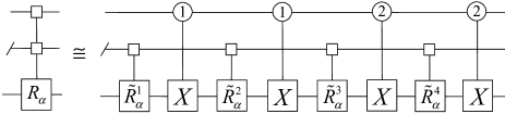
Figure 14: First step decomposition of a uniformly multifold controlled $R^{(ij)}_{\alpha}$ rotation.

The quantum circuit implementing ternary uniformly two-fold controlled $R_{\alpha}$ rotation is shown in Fig. 12. It has also been verified by matrix computing.

References

- (1) A. D. Greentree, S. G. Schirmer, F. Green, L. C. L. Hollenberg, A. R. Hamilton, and R. G. Clark, Phys. Rev. Lett. 92, 097901 (2004).
- (2) A. Muthukrishnan and C. R. Stroud, Jr., Phys. Rev. A 62, 052309 (2000).
- (3) A. B. Klimov, R. Guzmán, J. C. Retamal, and C.Saavedra, Phys. Rev. A 67, 062313 (2003).
- (4) S. S. Bullock, D. P. O’Leary, and G. K. Brennen, Phys. Rev. Lett. 94, 230502 (2005).
- (5) G. K. Brennen, S. S. Bullock, and D. P. O’Leary, Quant. Inf. Comp. 6, 436 (2006).
- (6) X. G. Wang, B. C. Sanders, and D. W. Berry, Phys. Rev. A 67, 042323 (2003).
- (7) B. P. Lanyon, M. Barbieri, M. P. Almeida, T. Jennewein, T. C. Ralph, K. J. Resch, G. J. Pryde, J. L. O’Brien, A. Gilchrist, and A. G. White, Nat. Phys. 5, 134 (2009).
- (8) M. Neeley, M. Ansmann, R. C. Bialczak, M. Hofheinz, E. Lucero, A. D. O’Connell, D. Sank, H. Wang, J. Wenner, A. N. Cleland, M. R. Geller, and J. M. Martinis, Science 325, 722 (2009).
- (9) R. Bianchetti, S. Filipp, M. Baur, J. M. Fink, C. Lang, L. Steffen, M. Boissonneault, A. Blais, and A. Wallraff, Phys. Rev. Lett. 105, 223601 (2010).
- (10) J. L. Brylinski and R. Brylinski, Mathematics of Quantum Computation (CRC Press, Boca Raton,FL, 2002).
- (11) M. J. Bremner, C. M. Dawson, J. L. Dodd, A. Gilchrist, A. W. Harrow, D. Mortimer, M. A. Nielsen, and T. J.Osborne, Phys. Rev. Lett. 89, 247902 (2002).
- (12) A. Barenco, C. H. Bennett, R. Cleve, D. P. DiVincenzo, N. Margolus, P. Shor, T. Sleator, J. A. Smolin, and H. Weinfurter, Phys. Rev. A 52, 3457 (1995).
- (13) J. J. Vartiainen, M. Möttönen, and M. M. Salomaa, Phys. Rev. Lett. 92, 177902 (2004).
- (14) M. Möttönen, J. J. Vartiainen, V. Bergholm, and M. M. Salomaa, Phys. Rev. Lett. 93, 130502 (2004).
- (15) G. Vidal and C. M. Dawson, Phys. Rev. A 69, 010301 (2004).
- (16) F. Vatan and C. Williams, Phys. Rev. A 69, 032315 (2004).
- (17) V. V. Shende, I. L. Markov, and S. S. Bullock, Phys. Rev. A 69, 062321(2004).
- (18) V. Bergholm, J. J. Vartiainen, M. Möttönen, and M. M. Salomaa, Phys. Rev. A 71, 052330 (2005).
- (19) Y. S. Zhang, M. Y. Ye, and G. C. Guo, Phys. Rev. A 71, 062331 (2005).
- (20) V. V. Shende, S. S. Bullock, and I. L. Markov, IEEE. Trans on CAD, 25, 1000 (2006).
- (21) H. R. Wei, Y. M. Di, and J. Zhang, Chin. Phys. Lett. 25, 3107 (2008).
- (22) H. R. Wei and Y. M. Di, Quant. Info. and Comp. 12, 0262 (2012).
- (23) K. G. H. Vollbrecht and R. F. Werner, J. Math. Phys. 41, 6772 (2000).
- (24) S. Helgason, Differential Geometry, Lie Groups and Symmetric Spaces ( Academic, New York, 1978).
- (25) J. I. Cirac and P. Zoller, Phys. Rev. Lett. 74, 4091 (1995).
- (26) C. Monroe, D. M. Meekhof, B. E. King, W. M. Itano, and D. J. Wineland, Phys. Rev. Lett. 75, 4714 (1995).
- (27) F. Schmidt-Kaler, H. Häffner, M. Riebe, S. Gulde, G. P. T. Lancaster, T. Deuschle, C. Becher, C. F. Roos, J. Eschner, and R. Blatt, Nature (London) 422, 408 (2003).
- (28) J. L. O’Brien, G. J. Pryde, A. G. White, T. C. Ralph, and D. Branning, Nature (London) 426, 264 (2003).
- (29) S. Gasparoni, J. W. Pan, P. Walther, T. Rudolph, and A. Zeilinger, Phys. Rev. Lett. 93, 020504 (2004).
- (30) R. Okamoto, H. F. Hofmann, S. Takeuchi, and K. Sasaki, Phys. Rev. Lett. 95, 210506 (2005).
- (31) A. Galiautdinov, Phys. Rev. A 75, 052303 (2007).
- (32) A. Galiautdinov, Phys. Rev. A 79, 042316 (2009).
- (33) T. Yamamoto, Y. A. Pashkin, O. Astafiev, Y. Nakamura, and J. S. Tsai, Nature (London) 425, 941 (2003).
- (34) J. Majer, J. M. Chow, J. M. Gambetta, J. Koch, B. R. Johnson, J. A. Schreier, L. Frunzio, D. I. Schuster, A. A. Houck, A. Wallraff, A. Blais, M. H. Devoret, S. M. Girvin, and R. J. Schoelkopf, Nature (London) 449, 443 (2007).
- (35) J. H. Plantenberg, P. C. de Groot, C. J. P. M. Harmans, and J. E. Mooij, Nature (London) 447, 836 (2007).
- (36) L. Isenhower, E. Urban, X. L. Zhang, A. T. Gill, T. Henage, T. A. Johnson, T. G. Walker, and M. Saffman, Phys. Rev. Lett. 104, 010503 (2010).
- (37) M. A. Nielsen and I. L. Chuang, Quantum Computation and Quantum Information (Cambridge University Press, UK, Cambridge, 2000).
- (38) H. Häffner, C. F. Roos, and R. Blatt, Phys. Reports 469, 155 (2008).
- (39) C. C. Paige and M. Wei, Linear Algebra Appl. 208/209, 303 (1994).
- (40) S. S. Bullock and I. L. Markov, Quant. Info. and Comp. 4, 027 (2004).