Inference for modulated stationary processes

Abstract

We study statistical inferences for a class of modulated stationary processes with time-dependent variances. Due to non-stationarity and the large number of unknown parameters, existing methods for stationary, or locally stationary, time series are not applicable. Based on a self-normalization technique, we address several inference problems, including a self-normalized central limit theorem, a self-normalized cumulative sum test for the change-point problem, a long-run variance estimation through blockwise self-normalization, and a self-normalization-based wild bootstrap. Monte Carlo simulation studies show that the proposed self-normalization-based methods outperform stationarity-based alternatives. We demonstrate the proposed methodology using two real data sets: annual mean precipitation rates in Seoul from 1771–2000, and quarterly U.S. Gross National Product growth rates from 1947–2002.

and

1 Introduction

In time series analysis, stationarity requires that dependence structure be sustained over time, and thus we can borrow information from one time period to study model dynamics over another period; see Fan and Yao [20] for nonparametric treatments and Lahiri [29] for various resampling and block bootstrap methods. In practice, however, many climatic, economic and financial time series are non-stationary and therefore challenging to analyze. First, since dependence structure varies over time, information is more localized. Second, non-stationary processes often require extra parameters to account for time-varying structure. One way to overcome these issues is to impose certain local stationarity; see, for example, Dahlhaus [15] and Adak [1] for spectral representation frameworks and Dahlhaus and Polonik [16] for a time domain approach.

In this article we study a class of modulated stationary processes (see Adak [1])

$$X_{i}=\mu+\sigma_{i}e_{i},\qquad i=1,\ldots,n,$$ (1)

where $e_{i}$ are stationary time series with zero mean, and $\sigma_{i}>0$ are unknown constants adjusting for time-dependent variances. Then $X_{i}$ oscillates around the constant mean $\mu$, whereas its variance changes over time in an unknown manner. In the special case of $\sigma_{i}\equiv 1$, (1) reduces to stationary case. If $\sigma_{i}=s(i/n)$ for a Lipschitz continuous function $s(t)$ on $[0,1]$, then (1) is locally stationary. For the general non-stationary case (1), the number of unknown parameters is larger than the number of observations, and it is infeasible to estimate $\sigma_{i}$. Due to non-stationarity and the large number of unknown parameters, existing methods that are developed for (locally) stationary processes are not applicable, and our main purpose is to develop new statistical inference techniques.

First, we establish a uniform strong approximation result which can be used to derive a self-normalized central limit theorem (CLT) for the sample mean $\bar{X}$ of (1). For stationary case $\sigma_{i}\equiv 1$, by Fan and Yao [20], under mild mixing conditions,

$$\sqrt{n}(\bar{X}-\mu)\Rightarrow N(0,\tau^{2}),\qquad\mbox{where }\tau^{2}=\gamma_{0}+2\sum^{\infty}_{k=1}\gamma_{k}\mbox{ and }\gamma_{k}=\operatorname{Cov}(e_{i},e_{i+k}).$$ (2)

For the modulated stationary case (1), it is non-trivial whether $\sqrt{n}(\bar{X}-\mu)$ has a CLT without imposing further assumptions on $\sigma_{i}$ and the dependence structure of $e_{i}$. Moreover, even when the latter CLT exists, it is difficult to estimate the limiting variance due to the large number of unknown parameters; see De Jong and Davidson [18] for related work assuming a near-epoch dependent mixing framework. Zhao [41] studied confidence interval construction for $\mu$ in (1) by assuming a block-wise asymptotically equal cumulative variance assumption. The latter assumption is rather restrictive and essentially requires that block averages be asymptotically independent and identically distributed (i.i.d.). In this article, we deal with the more general setting (1). Under a strong invariance principle assumption, we establish a self-normalized CLT with the self-normalizing constant adjusting for time-dependent non-stationarity. The obtained CLT is an extension of the classical CLT for i.i.d. data or stationary time series to modulated stationary processes. Furthermore, we extend the idea to linear combinations of means over different time periods, which allows us to address inference regarding mean levels over multiple time periods.

Second, we study the wild bootstrap for modulated stationary processes. Since the seminal work of Efron [19], a great deal of research has been done on the bootstrap under various settings, ranging from bootstrapping for i.i.d. data in Efron [19], wild bootstrapping for independent observations with possibly non-constant variances in Wu [39] and Liu [30], to various block bootstrapping and resampling methods for stationary time series in Künsch [27], Politis and Romano [34], Bühlmann [12] and the monograph Lahiri [29]. With the established self-normalized CLT, we propose a wild bootstrap procedure that is tailored to deal with modulated stationary processes: the dependence is removed through a scaling factor, and the non-constant variance structure of the original data is preserved in the wild bootstrap data-generating mechanism. Our simulation study shows that the wild bootstrap method outperforms the widely used stationarity-based block bootstrap.

Third, we address change-point analysis. The change-point problem has been an active area of research; see Pettitt [32] for proportion changes in binary data, Horváth [25] for mean and variance changes in Gaussian observations, Bai and Perron [8] for coefficient changes in linear models, Aue et al. [6] for coefficient changes in polynomial regression with uncorrelated errors, Aue et al. [7] for mean change in time series with stationary errors, Shao and Zhang [37] for change-points for stationary time series and the monograph by Csörgő and Horváth [14] for more discussion. Most of these works deal with stationary and/or independent data. Hansen [24] studied tests for constancy of parameters in linear regression models with non-stationary regressors and conditionally homoscedastic martingale difference errors. Here we consider

$$H_{0}\colon\ X_{i}=\mu_{i}+\sigma_{i}e_{i},\mu_{1}=\cdots=\mu_{n},\qquad H_{a}\colon\ \mu_{1}=\cdots=\mu_{J}\not=\mu_{J+1}=\cdots=\mu_{n},$$ (3)

where $J$ is an unknown change point. The aforementioned works mainly focused on detecting changes in mean while the error variance is constant. On the other hand, researchers have also realized the importance of the variance/covariance structure in change point analysis. For example, Inclán and Tiao [26] studied change in variance for independent data, and Aue et al. [5] and Berkes, Gombay and Horváth [10] considered change in covariance for time series data. To our knowledge, there has been almost no attempt to advance change point analysis under the non-constant variances framework in (3). Andrews [4] studied change point problem under near-epoch dependence structure that allows for non-stationary processes, but his Assumption 1(c) on page 830 therein essentially implies that the process has constant variance. The popular cumulative sum (CUSUM) test is developed for stationary time series and does not take into account the time-dependent variances. Using the self-normalization idea, we propose a self-normalized CUSUM test and a wild bootstrap method to obtain its critical value. Our empirical studies show that the usual CUSUM tests tend to over-reject the null hypothesis in the presence of non-constant variances. By contrast, the self-normalized CUSUM test yields size close to the nominal level.

Fourth, we estimate the long-run variance $\tau^{2}$ in (2). Long-run variance plays an essential role in statistical inferences involving time series. Most works in the literature deal with stationary processes through various block bootstrap and subsampling approaches; see Carlstein [13], Künsch [27], Politis and Romano [34], Götze and Künsch [21] and the monograph Lahiri [29]. De Jong and Davidson [18] established the consistency of kernel estimators of covariance matrices under a near epoch dependent mixing condition. Recently, Müller [31] studied robust long-run variance estimation for locally stationary process. For model (1), the error process $\{e_{i}\}$ is contaminated with unknown standard deviations $\{\sigma_{i}\}$, and we apply blockwise self-normalization to remove non-stationarity, resulting in asymptotically stationary blocks.

Fifth, the proposed methods can be extended to deal with the linear regression model

$$X_{i}=U_{i}\beta+\sigma_{i}e_{i},$$ (4)

where $U_{i}=(u_{i,1},\ldots,u_{i,p})$ are deterministic covariates, and $\beta=(\beta_{1},\ldots,\beta_{p})^{\prime}$ is the unknown column vector of parameters. For $p=2$, Hansen [23] established the asymptotic normality of the least-squares estimate of the slope parameter under a fairly general framework of non-stationary errors. While Hansen [23] assumed that the errors form a martingale difference array so that they are uncorrelated, the framework in (4) is more general in that it allows for correlations. On the other hand, Hansen [23] allowed the conditional volatilities to follow an autoregressive model, hence introducing stochastic volatilities. Phillips, Sun and Jin [33] considered (4) for stationary errors, and their approach is not applicable here due to the unknown non-constant variances $\sigma^{2}_{i}$. In Section 2.6 we consider self-normalized CLT for the least-squares estimator of $\beta$ in (4). In the polynomial regression case $u_{i,r}=(i/n)^{r-1}$, Aue et al. [6] studied a likelihood-based test for constancy of $\beta$ in (4) for uncorrelated errors with constant variance. Due to the presence of correlation and time-varying variances, it is more challenging to study the change point problem for (4) and this is beyond the scope of this article.

The rest of this article is organized as follows. We present theoretical results in Section 2. Sections 3–4 contain Monte Carlo studies and applications to two real data sets.

2 Main results

For sequences $\{a_{n}\}$ and $\{b_{n}\}$, write $a_{n}=\mathrm{O}(b_{n})$, $a_{n}=\mathrm{o}(b_{n})$ and $a_{n}\asymp b_{n}$, respectively, if $|a_{n}/b_{n}|<c_{1}$, $a_{n}/b_{n}\to 0$ and $c_{2}<|a_{n}/b_{n}|<c_{3}$, for some constants $0<c_{1},c_{2},c_{3}<\infty$. For $q>0$ and a random variable $e$, write $e\in\mathcal{L}^{q}$ if $\|e\|_{q}:=\{E(|e|^{q})\}^{1/q}<\infty$.

2.1 Uniform approximations for modulated stationary processes

In (1), assume without loss of generality that $E(e_{i})=0$ and $E(e^{2}_{i})=1$ so that $\{e_{i}\}$ and $\{e^{2}_{i}-1\}$ are centered stationary processes. With the convention $S_{0}=S^{*}_{0}=0$, define

$$S_{i}=\sum^{i}_{j=1}e_{j}\quad\mbox{and}\quad S^{*}_{i}=\sum^{i}_{j=1}(e^{2}_{j}-1),\qquad i=1,2,\ldots.$$ (5)

Assumption 2.1.

There exist standard Brownian motions $\{B_{t}\}$ and $\{B^{*}_{t}\}$ such that

$$\max_{1\leq i\leq n}|S_{i}-\tau B_{i}|=\mathrm{o}_{\mathrm{a.s.}}(\Delta_{n})\quad\mbox{and}\quad\max_{1\leq i\leq n}|S^{*}_{i}-\tau^{*}B^{*}_{i}|=\mathrm{o}_{\mathrm{a.s.}}(\Delta_{n}),$$ (6)

where $\Delta_{n}$ is the approximation error, $\tau^{2}$ and $\tau^{*2}$ are the long-run variances of $\{e_{i}\}$ and $\{e^{2}_{i}-1\}$, respectively. Further assume $\tau^{2}>0$ to avoid the degenerate case $\tau^{2}=0$.

The uniform approximations in (6) are generally called strong invariance principle. The two Brownian motions $\{B_{t}\}$ and $\{B^{*}_{t}\}$ may be defined on different probability spaces and hence are not jointly distributed, which is not an issue because our argument does not depend on their joint distribution. To see how to use (6), under $H_{0}$ in (3), consider

$$F_{j}=j(\underline{X}_{j}-\mu)\quad\mbox{and}\quad\underline{V}^{2}_{j}=\sum^{j}_{i=1}(X_{i}-\underline{X}_{j})^{2},\qquad\mbox{where }\underline{X}_{j}=j^{-1}\sum^{j}_{i=1}X_{i}.$$ (7)

Theorem 2.1 below presents uniform approximations for $F_{j}$ and $V^{2}_{j}$. Define

$$r_{n} = |\sigma_{n}|+\sum^{n}_{i=2}|\sigma_{i}-\sigma_{i-1}|\quad\mbox{and}\quad r^{*}_{n}=|\sigma^{2}_{n}|+\sum^{n}_{i=2}|\sigma^{2}_{i}-\sigma^{2}_{i-1}|,$$ (8)

$$\Sigma^{2}_{j} = \sum^{j}_{i=1}\sigma^{2}_{i}\quad\mbox{and}\quad\Sigma^{*2}_{j}=\Biggl{(}\sum^{j}_{i=1}\sigma^{4}_{i}\Biggr{)}^{1/2}.\vspace*{-2pt}$$ (9)

Theorem 2.1

Let (6) hold. For any $c\in(0,1]$, the following uniform approximations hold:

$$\max_{cn\leq j\leq n}\Biggl{|}F_{j}-\tau\sum^{j}_{i=1}\sigma_{i}(B_{i}-B_{i-1})\Biggr{|}=\mathrm{O}_{\mathrm{a.s.}}(r_{n}\Delta_{n}),$$ (10)

$$\max_{cn\leq j\leq n}|\underline{V}^{2}_{j}-\Sigma^{2}_{j}|=\mathrm{O}_{\mathrm{p}}\{(r^{2}_{n}\Delta^{2}_{n}+\Sigma^{2}_{n})/n+\Sigma^{*2}_{n}+r^{*}_{n}\Delta_{n}\}.\vspace*{-2pt}$$ (11)

Theorem 2.1 provides quite general results under (6). We now discuss sufficient conditions for (6). Shao [36] obtained sufficient mixing conditions for (6). In this article, we briefly introduce the framework in Wu [40]. Assume that $e_{i}$ has the causal representation $e_{i}=G(\ldots,\varepsilon_{i-1},\varepsilon_{i})$, where $\varepsilon_{i}$ are i.i.d. innovations, and $G$ is a measurable function such that $e_{i}$ is well defined. Let $\{\varepsilon_{i}^{\prime}\}_{i\in\mathbb{Z}}$ be an independent copy of $\{\varepsilon_{i}\}_{i\in\mathbb{Z}}$. Assume

$$\sum_{i=1}^{\infty}i\|e_{i}-e^{\prime}_{i}\|_{8}<\infty,\qquad\mbox{where }e^{\prime}_{i}=G(\ldots,\varepsilon_{-1},\varepsilon_{0}^{\prime},\varepsilon_{1},\ldots,\varepsilon_{i-1},\varepsilon_{i}).$$ (12)

Proposition 2.1 below follows from Corollary 4 in Wu [40].

Proposition 2.1.

Assume that (12) holds. Then (6) holds with $\Delta_{n}=n^{1/4}\log(n)$, the optimal rate up to a logarithm factor.

For linear process $e_{i}=\sum^{\infty}_{j=0}a_{j}\varepsilon_{i-j}$ with $\varepsilon_{i}\in\mathcal{L}^{8}$ and $E(\varepsilon_{i})=0$, $\|e_{i}-e^{\prime}_{i}\|_{8}=\|\varepsilon_{0}-\varepsilon^{\prime}_{0}\|_{8}|a_{i}|$. If $\sum^{\infty}_{i=1}i|a_{i}|<\infty$, then (6) holds with $\Delta_{n}=n^{1/4}\log(n)$. For many nonlinear time series, $\|e_{i}-e^{\prime}_{i}\|_{8}$ decays exponentially fast and hence (12) holds; see Section 3.1 of Wu [40]. From now on we assume (6) holds with $\Delta_{n}=n^{1/4}\log(n)$.

Remark 2.0.

If $e_{i}$ are i.i.d. with $E(e_{i})=0$ and $e_{i}\in\mathcal{L}^{q}$ for some $2<q\leq 4$, the celebrated “Hungarian embedding” asserts that $\sum^{i}_{j=1}e_{j}$ satisfies a strong invariance principle with the optimal rate $\mathrm{o}_{\mathrm{a.s.}}(n^{1/q})$. Thus, it is necessary to have the moment assumption $e_{i}\in\mathcal{L}^{8}$ in Proposition 2.1 in order to ensure strong invariance principles for both $S_{i}$ and $S^{*}_{i}$ in (5) with approximation rate $n^{1/4}\log(n)$. On the other hand, one can relax the moment assumption by loosening the approximation rate. For example, by Corollary 4 in Wu [40], assume $e_{i}\in\mathcal{L}^{2q}$ for some $q>2$ and $\sum_{i=1}^{\infty}i\|e_{i}-e_{i}^{*}\|_{2q}<\infty$, then (6) holds with $\Delta_{n}=n^{1/\min(q,4)}\log(n)$.

As shown in Examples 2.1–2.3 below, $r_{n}$ and $r^{*}_{n}$ in (8) often have tractable bounds.

Example 2.1.

If $\sigma_{i}$ is non-decreasing in $i$, then $\sigma_{n}\leq r_{n}\leq 2\sigma_{n}$ and $\sigma^{2}_{n}\leq r^{*}_{n}\leq 2\sigma^{2}_{n}$. If $\sigma_{i}$ is non-increasing in $i$, then $r_{n}=\sigma_{1}$ and $r^{*}_{n}=\sigma^{2}_{1}$. If $\sigma_{i}$ are piecewise constants with finitely many pieces, then $r_{n},r^{*}_{n}=\mathrm{O}(1)$.

Example 2.2.

Let $\sigma_{i}=s(i/n^{\gamma})$ for $\gamma\in[0,1]$ and a Lipschitz continuous function $s(t),t\in[0,\infty),\sup_{t\in[0,\infty)}s(t)<\infty$. Then $r_{n},r^{*}_{n}=\mathrm{O}(n^{1-\gamma})$. If $\gamma=1$, we obtain a locally stationary case with the time window $i/n\in[0,1]$; if $\gamma\in[0,1)$, we have the infinite time window $[0,\infty)$ as $n/n^{\gamma}\to\infty$, which may be more reasonable for data with a long time horizon.

Example 2.3.

If $\sigma_{i}=i^{\beta}L(i)$ for a slowly varying function $L(\cdot)$ such that $L(cx)/L(x)\to 1$ as $x\to\infty$ for all $c>0$. Then we can show $r_{n}=\mathrm{O}\{n^{\beta}L(n)\}$ or $\mathrm{O}(1)$ and $r^{*}_{n}=\mathrm{O}\{n^{2\beta}L^{2}(n)\}$ or $\mathrm{O}(1)$, depending on whether $\beta>0$ or $\beta<0$. For the boundary case $\beta=0$, assume $L(i+1)/L(i)=1+\mathrm{O}(1/i)$ uniformly, then $r_{n}=L(n)+\mathrm{O}(1)\sum^{n}_{i=2}L(i)/i=\mathrm{O}\{\log(n)\times\max_{1\leq i\leq n}L(i)\}$. Similarly, $r^{*}_{n}=\mathrm{O}\{\log(n)\max_{1\leq i\leq n}L^{2}(i)\}$.

2.2 Self-normalized central limit theorem

In this section we establish a self-normalized CLT for the sample average $\bar{X}$. To understand how non-stationarity makes this problem difficult, elementary calculation shows

$$\operatorname{Var}\bigl{\{}\sqrt{n}(\bar{X}-\mu)\bigr{\}}=\frac{\gamma_{0}}{n}\sum^{n}_{i=1}\sigma^{2}_{i}+\frac{2}{n}\sum_{1\leq i<j\leq n}\sigma_{i}\sigma_{j}\gamma_{j-i}:=\tau^{2}_{n},$$ (13)

where $\gamma_{k}=\operatorname{Cov}(e_{0},e_{k})$. In the stationary case $\sigma_{i}\equiv 1$, under condition $\sum^{\infty}_{k=0}|\gamma_{k}|<\infty$, $\tau^{2}_{n}\to\tau^{2}$, the long-run variance in (2). For non-constant variances, it is difficult to deal with $\tau^{2}_{n}$ directly, due to the large number of unknown parameters and complicated structure. See De Jong and Davidson [18] for a kernel estimator of $\tau^{2}_{n}$ under a near-epoch dependent mixing framework.

To attenuate the aforementioned issue, we apply the uniform approximations in Theorem 2.1. Assume that (14) below holds. Note that the increments $B_{i}-B_{i-1}$ of standard Brownian motions are i.i.d. standard normal random variables. By (10), $n(\bar{X}-\mu)$ is equivalent to $N(0,\tau^{2}\Sigma^{2}_{n})$ in distribution. By (11), $\underline{V}_{n}/\Sigma_{n}\to 1$ in probability. By Slutsky’s theorem, we have Proposition 2.2.

Proposition 2.2.

Let (6) hold with $\Delta_{n}=n^{1/4}\log(n)$. For $r_{n},r^{*}_{n},\Sigma^{2}_{n},\Sigma^{*2}_{n}$ in (8)–(9), assume

$$\delta_{n}=r_{n}\Delta_{n}/\Sigma_{n}+(r^{*}_{n}\Delta_{n}+\Sigma^{*2}_{n})/\Sigma^{2}_{n}\to 0.$$ (14)

Recall $\underline{V}_{n}^{2}$ in (7). Then as $n\to\infty$, $n(\bar{X}-\mu)/\underline{V}_{n}\Rightarrow N(0,\tau^{2})$. Consequently, a $(1-\alpha)$ asymptotic confidence interval for $\mu$ is $\bar{X}\pm z_{\alpha/2}\hat{\tau}\underline{V}_{n}/n$, where $\hat{\tau}$ is a consistent estimate of $\tau$ (Section 2.5 below), and $z_{\alpha/2}$ is $(1-\alpha/2)$ standard normal quantile.

Proposition 2.2 is an extension of the classical CLT for i.i.d. data or stationary processes to modulated stationary processes. If $X_{i}$ are i.i.d., then $n(\bar{X}-\mu)/\underline{V}_{n}\Rightarrow N(0,1)$. In Proposition 2.2, $\tau^{2}$ can be viewed as the variance inflation factor due to the dependence of $\{e_{i}\}$. For stationary data, the sample variance $\underline{V}^{2}_{n}/n$ is a consistent estimate of the population variance. Here, for non-constant variances case (1), by (11) in Theorem 2.1, $\underline{V}^{2}_{n}/n$ can be viewed as an estimate of the time-average “population variance” $\Sigma^{2}_{n}/n$. So, we can interpret the CLT in Proposition 2.2 as a self-normalized CLT for modulated stationary processes with the self-normalizing term $\underline{V}_{n}$, adjusting for non-stationarity due to $\sigma_{1},\ldots,\sigma_{n}$ and $\tau^{2}$, accounting for dependence of $\{e_{i}\}$. Clearly, parameters $\sigma_{1},\ldots,\sigma_{n}$ are canceled out through self-normalization. Finally, condition (14) is satisfied in Example 2.2 with $\gamma>3/4$ and Example 2.3 with $\beta>-1/4$.

In classical statistics, the width of confidence intervals usually shrinks as sample size increases. By Proposition 2.2 and Theorem 2.1, the width of the constructed confidence interval for $\mu$ is proportional to $\underline{V}_{n}/n$ or, equivalently, $\Sigma_{n}/n$. Thus, a necessary and sufficient condition for shrinking confidence interval is $\sum^{n}_{i=1}\sigma^{2}_{i}/n^{2}\to 0$, which is satisfied if $\sigma_{i}=\mathrm{o}(\sqrt{i})$. An intuitive explanation is as follows. For i.i.d. data, sample mean converges at a rate of $\mathrm{O}(\sqrt{n})$. In (1), if $\sigma_{i}$ grows faster than $\mathrm{O}(\sqrt{i})$, the contribution of a new observation is negligible relative to its noise level.

Example 2.4.

If $\sigma_{i}\asymp i^{\beta}$ with $\beta\in[0,1/2)$, the length of confidence interval is proportional to $\Sigma_{n}/n\asymp n^{\beta-1/2}$. In particular, if $c_{1}<\sigma_{i}<c_{2}$ for some positive constants $c_{1}$ and $c_{2}$, then $\Sigma_{n}/n$ achieves the optimal rate $\mathrm{O}(n^{-1/2})$. If $\sigma_{i}\asymp\log(i)$, then $\Sigma_{n}/n\asymp\log(n)/\sqrt{n}$.

The same idea can be extended to linear combinations of means over multiple time periods. Suppose we have observations from $k$ consecutive time periods $\mathcal{T}_{1},\ldots,\mathcal{T}_{k}$, each of the form (1) with different means, denoted by $\mu_{1},\ldots,\mu_{k}$, and each having time-dependent variances. Let $\nu=\beta_{1}\mu_{1}+\cdots+\beta_{k}\mu_{k}$ for given coefficients $\beta_{1},\ldots,\beta_{k}$. For example, if we are interested in mean change from $\mathcal{T}_{1}$ to $\mathcal{T}_{2}$, we can take $\nu=\mu_{2}-\mu_{1}$; if we are interested in whether the increase from $\mathcal{T}_{3}$ to $\mathcal{T}_{4}$ is larger than that from $\mathcal{T}_{1}$ to $\mathcal{T}_{2}$, we can let $\nu=(\mu_{4}-\mu_{3})-(\mu_{2}-\mu_{1})$. Proposition 2.3 below extends Proposition 2.2 to multiple means.

Proposition 2.3.

Let $\nu=\beta_{1}\mu_{1}+\cdots+\beta_{k}\mu_{k}$. For $\mathcal{T}_{j}$, denote its sample size $n_{j}$ and its sample average $\bar{X}(j)$. Assume that (14) holds for each individual time period $\mathcal{T}_{j}$ and, for simplicity, that $n_{1},\ldots,n_{k}$ are of the same order. Then

$$\frac{\sum^{k}_{j=1}\beta_{j}\bar{X}(j)-\nu}{\Lambda_{n}}\Rightarrow N(0,\tau^{2}),\qquad\mbox{where }\Lambda^{2}_{n}=\sum^{k}_{j=1}\biggl{\{}\frac{\beta^{2}_{j}}{n^{2}_{j}}\sum_{i\in\mathcal{T}_{j}}[X_{i}-\bar{X}(j)]^{2}\biggr{\}}.$$

2.3 Wild bootstrap for self-normalized statistic

Recall $\sigma_{i}e_{i}$ in (1). Suppose we are interested in the self-normalized statistic

$$H_{n}=\frac{\sum^{n}_{i=1}\sigma_{i}e_{i}}{\sqrt{\sum^{n}_{i=1}\sigma^{2}_{i}e^{2}_{i}}}.$$

For problems with small sample sizes, it is natural to use bootstrap distribution instead of the convergence $H_{n}\Rightarrow N(0,\tau^{2})$ in Proposition 2.2. Wu [39] and Liu [30] have pioneered the work on the wild bootstrap for independent data with non-identical distributions. We shall extend their wild bootstrap procedure to the modulated stationary process (1).

Let $\{\alpha_{i}\}$ be i.i.d. random variables independent of $\{e_{i}\}$ satisfying $\alpha_{i}\in\mathcal{L}^{3},E(\alpha_{i})=0,E(\alpha^{2}_{i})=1$. Define the self-normalized statistic based on the following new data:

$$H^{*}_{n}=\frac{\sum^{n}_{i=1}\xi_{i}}{\sqrt{\sum^{n}_{i=1}(\xi_{i}-\bar{\xi})^{2}}},\qquad\mbox{where }\xi_{i}=\sigma_{i}e_{i}\alpha_{i}\mbox{ and }\bar{\xi}=\frac{\xi_{1}+\cdots+\xi_{n}}{n}.$$

Clearly, $\xi_{i}$ inherits the non-stationarity structure of $\sigma_{i}e_{i}$ by writing $\xi_{i}=\sigma_{i}e^{*}_{i}$ with $e^{*}_{i}=e_{i}\alpha_{i}$. On the other hand, for the new error process $\{e^{*}_{i}\}$, $E(e^{*2}_{i})=E(e^{2}_{i})=1$ and $\operatorname{Cov}(e^{*}_{i},e^{*}_{j})=0$ for $i\neq j$. Thus, $\{e^{*}_{i}\}$ is a white noise sequence with long-run variance one. By Proposition 2.2, the scaled version $H_{n}/\tau\Rightarrow N(0,1)$ is robust against the dependence structure of $\{e_{i}\}$, so we expect that $H_{n}^{*}$ should be close to $H_{n}/\tau$ in distribution.

Theorem 2.2

Let the conditions in Proposition 2.2 hold. Further assume

$$\Biggl{(}\sum^{n}_{i=1}\sigma^{3}_{i}\Biggr{)}^{2}\Biggl{(}\sum^{n}_{i=1}\sigma^{2}_{i}\Biggr{)}^{-3}\to 0.$$ (15)

Let $\hat{\tau}$ be a consistent estimate of $\tau$. Denote by $\mathbb{P}^{*}$ the conditional law given $\{e_{i}\}$. Then

$$\sup_{x\in\mathbb{R}}|\mathbb{P}^{*}(H^{*}_{n}\leq x)-\mathbb{P}(H_{n}/\hat{\tau}\leq x)|\to 0,\qquad\mbox{in probability}.$$ (16)

Theorem 2.2 asserts that, $H^{*}_{n}$ behaves like the scaled version $H_{n}/\hat{\tau}$, with the scaling factor $\hat{\tau}$ coming from the dependence of $\{e_{i}\}$. Here we use the sample mean $\bar{X}$ in (1) to illustrate a wild bootstrap procedure to obtain the distribution of $n(\bar{X}-\mu)/(\tau\underline{V}_{n})$ in Proposition 2.2.

1. [(iii)]

2. Apply the method in Section 2.5 to $X_{1},\ldots,X_{n}$ to obtain a consistent estimate $\hat{\tau}$ of $\tau$.

3. Subtract the sample mean $\bar{X}$ from data to obtain $\epsilon_{i}=X_{i}-\bar{X},i=1,\ldots,n$.

4. Generate i.i.d. random variables $\alpha_{1},\ldots,\alpha_{n}$ satisfying $E(\alpha_{i})=0,E(\alpha^{2}_{i})=1$.

5. Based on $\epsilon_{i}$ in (ii) and $\alpha_{i}$ in (iii), generate bootstrap data $\xi^{b}_{i}=\epsilon_{i}\alpha_{i}$, and compute

   $$H^{b}_{n}=\frac{\sum^{n}_{i=1}\xi^{b}_{i}}{\hat{\tau}^{b}\sqrt{\sum^{n}_{i=1}(\xi^{b}_{i}-\bar{\xi}^{b})^{2}}},$$

   where $\hat{\tau}^{b}$ is a long-run variance estimate (see Section 2.5) for bootstrap data $\xi^{b}_{i}$.

6. Repeat (iii)–(iv) many times and use the empirical distribution of those realizations of $H^{b}_{n}$ as the distribution of $n(\bar{X}-\mu)/(\tau\underline{V}_{n})$.

The proposed wild bootstrap is an extension of that in Liu [30] for independent data to modulated stationary case, and it has two appealing features. First, the scaling factor $\hat{\tau}$ makes the statistic independent of the dependence structure. Second, the bootstrap data-generating mechanism is adaptive to unknown time-dependent variances $\{\sigma^{2}_{i}\}$. For the distribution of $\alpha_{i}$ in step (iii), we use $\mathbb{P}(\alpha_{i}=-1)=\mathbb{P}(\alpha_{i}=1)=1/2$, which has some desirable properties. For example, it preserves the magnitude and range of the data. As shown by Davidson and Flachaire [17], for certain hypothesis testing problems in linear regression models with symmetrically distributed errors, the bootstrap distribution is exactly equal to that of the test statistic; see Theorem 1 therein.

For the purpose of comparison, we briefly introduce the widely used block bootstrap for a stationary time series $\{X_{i}\}$ with mean $\mu$. By (2), $\sqrt{n}(\bar{X}-\mu)\Rightarrow N(0,\tau^{2})$. Suppose that we want to bootstrap the distribution of $\sqrt{n}(\bar{X}-\mu)$. Let $k_{n},\ell_{n},\mathcal{I}_{1},\ldots,\mathcal{I}_{\ell_{n}}$ be defined as in Section 2.5 below. The non-overlapping block bootstrap works in the following way:

1. [(iii)]

2. Take a simple random sample of size $\ell_{n}$ with replacement from the blocks $\mathcal{I}_{1},\ldots,\mathcal{I}_{\ell_{n}}$, and form the bootstrap data $X^{b}_{1},\ldots,X^{b}_{n^{\prime}},n^{\prime}=k_{n}\ell_{n},$ by pooling together $X_{i}$s for which the index $i$ is within those selected blocks.

3. Let $\bar{X}^{b}$ be the sample average of $X^{b}_{1},\ldots,X^{b}_{n^{\prime}}$. Compute $\Xi_{n}=\sqrt{n^{\prime}}\{\bar{X}^{b}-E^{*}(\bar{X}^{b})\}$, where $E^{*}(\bar{X}^{b})=\sum^{n^{\prime}}_{i=1}X_{i}/n^{\prime}$ is the conditional expectation of $\bar{X}^{b}$ given $\{X_{i}\}$.

4. Repeat (i)–(ii) many times and use the empirical distribution of $\Xi_{n}$’s as the distribution of $\sqrt{n}(\bar{X}-\mu)$.

In step (ii), another choice is the studentized version $\tilde{\Xi}_{n}=\sqrt{n^{\prime}}\{\bar{X}^{b}-E^{*}(\bar{X}^{b})\}/\hat{\tau}^{b}$, where $\hat{\tau}^{b}$ is a consistent estimate of $\tau$ based on bootstrap data. Assuming stationarity and $k_{n}\to\infty$, the blocks are asymptotically independent and share the same model dynamics as the whole data, which validates the above block bootstrap. We refer the reader to Lahiri [29] for detailed discussions. For a non-stationary process, block bootstrap is no longer valid, because individual blocks are not representative of the whole data. By contrast, the proposed wild bootstrap is adaptive to unknown dependence and the non-constant variances structure.

2.4 Change point analysis: Self-normalized CUSUM test

To test a change point in the mean of a process $\{X_{i}\}$, two popular CUSUM-type tests (see Section 3 of Robbins et al. [35] for a review and related references) are

$$T^{1}_{n}=\max_{cn\leq j\leq(1-c)n}\frac{\hat{\tau}^{-1}|S_{X}(j)|}{\sqrt{j(1-j/n)}}\quad\mbox{and}\quad T^{2}_{n}=\max_{cn\leq j\leq(1-c)n}\hat{\tau}^{-1}|S_{X}(j)|,$$ (17)

where $\hat{\tau}^{2}$ is a consistent estimate of the long-run variance $\tau^{2}$ of $\{X_{i}\}$, and

$$S_{X}(j)=\biggl{(}1-\frac{j}{n}\biggr{)}\sum^{j}_{i=1}X_{i}-\frac{j}{n}\sum^{n}_{i=j+1}X_{i}.$$ (18)

Here $c>0$ ($c=0.1$ in our simulation studies) is a small number to avoid the boundary issue. For i.i.d. data, $j(1-j/n)$ is proportional to the variance of $S_{X}(j)$, so $T^{1}_{n}$ is a studentized version of $T^{2}_{n}$. For i.i.d. Gaussian data, $T^{1}_{n}$ is equivalent to likelihood ratio test; see Csörgő and Horváth [14]. Assume that, under null hypothesis,

$$\Biggl{\{}n^{-1/2}\sum^{\lfloor nt\rfloor}_{i=1}[X_{i}-E(X_{i})]\Biggr{\}}_{0\leq t\leq 1}\Rightarrow\tau\{B_{t}\}_{0\leq t\leq 1},\qquad\mbox{in the Skorohod space}$$ (19)

for a standard Brownian motion $\{B_{t}\}_{t\geq 0}$. The above convergence requires finite-dimensional convergence and tightness; see Billingsley [11]. By the continuous mapping theorem, $T^{1}_{n}\Rightarrow\max_{c\leq t\leq 1-c}|B_{t}-tB_{1}|/\sqrt{t(1-t)}$ and $T^{2}_{n}/\sqrt{n}\Rightarrow\max_{c\leq t\leq 1-c}|B_{t}-tB_{1}|$.

For the modulated stationary case (3), (19) is no longer valid. Moreover, since $T^{1}_{n}$ and $T^{2}_{n}$ do not take into account the time-dependent variances $\sigma^{2}_{i}$, an abrupt change in variances may lead to a false rejection of $H_{0}$ when the mean remains constant. For example, our simulation study in Section 3.3 shows that the empirical false rejection probability for $T^{1}_{n}$ and $T^{2}_{n}$ is about $10\%$ for nominal level $5\%$. To alleviate the issue of non-constant variances, we adopt the self-normalization approach as in previous sections. Recall $F_{j}$ and $\underline{V}_{j}$ in (7). For each fixed $cn\leq j\leq(1-c)n$, by Theorem 2.1 and Slutsky’s theorem, $F_{j}/\underline{V}_{j}\Rightarrow N(0,\tau^{2})$ in distribution, assuming the negligibility of the approximation errors. Therefore, the self-normalization term $\underline{V}_{j}$ can remove the time-dependent variances. In light of this, we can simultaneously self-normalize the two terms $\sum^{j}_{i=1}X_{i}$ and $\sum^{n}_{i=j+1}X_{i}$ in (18) and propose the self-normalized test statistic

$$T^{\mathrm{SN}}_{n}=\max_{cn\leq j\leq(1-c)n}\hat{\tau}^{-1}|T_{n}(j)|,\quad\mbox{where }T_{n}(j)=\frac{S_{X}(j)}{\sqrt{(1-j/n)^{2}\underline{V}^{2}_{j}+(j/n)^{2}\overline{V}^{2}_{j}}}.$$ (20)

Here, $\underline{V}^{2}_{j}$ is defined as in (7), $\overline{V}^{2}_{j}=\sum^{n}_{i=j+1}(X_{i}-\overline{X}_{j})^{2}$ with $\overline{X}_{j}=(n-j)^{-1}\sum^{n}_{i=j+1}X_{i}$.

Theorem 2.3

Assume (6) holds. Let $\delta_{n}\to 0$ be as in (14). Under $H_{0}$, we have

$$\max_{cn\leq j\leq(1-c)n}|T_{n}(j)-\tau\widetilde{T}_{n}(j)|=\mathrm{O}_{\mathrm{p}}(\delta_{n}),$$

where

$$\widetilde{T}_{n}(j)=\frac{(1-j/n)\sum^{j}_{i=1}\sigma_{i}(B_{i}-B_{i-1})-j/n\sum^{n}_{i=j+1}\sigma_{i}(B_{i}-B_{i-1})}{\sqrt{(1-j/n)^{2}\sum^{j}_{i=1}\sigma^{2}_{i}+(j/n)^{2}\sum^{n}_{i=j+1}\sigma^{2}_{i}}}.$$

By Theorem 2.3, under $H_{0}$, $T^{\mathrm{SN}}_{n}$ is asymptotically equivalent to $\max_{cn\leq j\leq(1-c)n}|\widetilde{T}_{n}(j)|$. Due to the self-normalization, for each $j$, the time-dependent variances are removed and $\widetilde{T}_{n}(j)\sim N(0,1)$ has a standard normal distribution. However, $\widetilde{T}_{n}(j)$ and $\widetilde{T}_{n}(j^{\prime})$ are correlated for $j\neq j^{\prime}$. Therefore, $\{\widetilde{T}_{n}(j)\}$ is a non-stationary Gaussian process with a standard normal marginal density. Due to the large number of unknown parameters $\sigma_{i}$, it is infeasible to obtain the null distribution directly. On the other hand, Theorem 2.3 establishes the fact that, asymptotically, the distribution of $T^{\mathrm{SN}}_{n}$ in (20) depends only on $\sigma_{1},\ldots,\sigma_{n}$ and is robust against the dependence structure of $\{e_{i}\}$, which motivates us to use the wild bootstrap method in Section 2.3 to find the critical value of $T^{\mathrm{SN}}_{n}$.

1. [(iii)]

2. Compute $T_{n}(j)$ and find $\hat{J}=\operatorname{argmax}_{cn\leq j\leq(1-c)n}|T_{n}(j)|$.

3. Divide the data into two blocks $X_{1},\ldots,X_{\hat{J}}$ and $X_{\hat{J}+1},\ldots,X_{n}$. Within each block, subtract the sample mean from the observations therein to obtain centered data. Pool all centered data together and denote them by $\epsilon_{1},\ldots,\epsilon_{n}$.

4. Based on $\epsilon_{1},\ldots,\epsilon_{n}$, obtain an estimate $\hat{\tau}$ of $\tau$. See Section 2.5 below.

5. Compute the test statistic $T^{\mathrm{SN}}_{n}$ in (20).

6. Based on $\epsilon_{i}$ in (ii), use the wild bootstrap method in Section 2.3 to generate synthetic data $\xi_{1},\ldots,\xi_{n}$, and use (i)–(iv) to compute the bootstrap test statistic $T^{b}_{n}$ based on the bootstrap data $\xi_{1},\ldots,\xi_{n}$.

7. Repeat (v) many times and find $(1-\alpha)$ quantile of those $T^{b}_{n}$s.

As argued in Section 2.3, the synthetic data-generating scheme (v) inherits the time-varying non-stationarity structure of the original data. Also, the statistic $T^{\mathrm{SN}}_{n}$ is robust against the dependence structure, which justifies the proposed bootstrap method. If $H_{0}$ is rejected, the change point is then estimated by $\hat{J}=\operatorname{argmax}_{cn\leq j\leq(1-c)n}|T_{n}(j)|$.

If there is no evidence to reject $H_{0}$, we briefly discuss how to apply the same methodology to test $\tilde{H}_{0}\colon\ \sigma_{1}=\cdots=\sigma_{J}\neq\sigma_{J+1}=\cdots=\sigma_{n}$, that is, whether there is a change point in the variances $\sigma^{2}_{i}$. By (1), we have $(X_{i}-\mu)^{2}=\sigma^{2}_{i}+\sigma^{2}_{i}\zeta_{i}$, where $\zeta_{i}=e^{2}_{i}-1$ has mean zero. Therefore, testing a change point in the variances $\sigma^{2}_{i}$ of $X_{i}$ is equivalent to testing a change point in the mean of the new data $\tilde{X}_{i}=(X_{i}-\bar{X})^{2}$.

2.5 Long-run variance estimation

To apply the results in Sections 2.2–2.4, we need a consistent estimate of the long-run variance $\tau^{2}$. Most existing works deal with stationary time series through various block bootstrap and subsampling approaches; see Lahiri [29] and references therein. Assuming a near-epoch dependent mixing condition, De Jong and Davidson [18] established the consistency of a kernel estimator of $\operatorname{Var}(\sum^{n}_{i=1}X_{i})$, and their result can be used to estimate $\tau^{2}_{n}$ in (13) for the CLT of $\sqrt{n}(\bar{X}-\mu)$. However, for the change point problem in Section 2.4, we need an estimator of the long-run variance $\tau^{2}$ of the unobservable process $\{e_{i}\}$, so the method in De Jong and Davidson [18] is not directly applicable.

To attenuate the non-stationarity issue, we extend the idea in Section 2.2 to blockwise self-normalization. Let $k_{n}$ be the block length. Denote by $\ell_{n}=\lfloor n/k_{n}\rfloor$ the largest integer not exceeding $n/k_{n}$. Ignore the boundary and divide $1,\ldots,n$ into $\ell_{n}$ blocks

$$\mathcal{I}_{j}=\{(j-1)k_{n}+1,\ldots,jk_{n}\},\qquad j=1,\ldots,\ell_{n}.$$ (21)

Recall the overall sample mean $\bar{X}$. For each block $j$, define the self-normalized statistic

$$D_{j}=\frac{k_{n}[\bar{X}(j)-\bar{X}]}{V(j)},\qquad\mbox{where }\bar{X}(j)=\frac{1}{k_{n}}\sum_{i\in\mathcal{I}_{j}}X_{i},V^{2}(j)=\sum_{i\in\mathcal{I}_{j}}[X_{i}-\bar{X}(j)]^{2}.$$ (22)

By Proposition 2.2, the self-normalized statistics $D_{1},\ldots,D_{\ell_{n}}\sim N(0,\tau^{2})$ are asymptotically i.i.d. Thus, we propose estimating $\tau^{2}$ by

$$\hat{\tau}^{2}=\frac{1}{\ell_{n}}\sum^{\ell_{n}}_{j=1}D^{2}_{j}.$$ (23)

As in (8)–(9), we define the quantities on block $j$

$$r(j) = |\sigma_{jk_{n}}|+\sum_{i\in\mathcal{I}_{j}}|\sigma_{i}-\sigma_{i-1}|\quad\mbox{and}\quad r^{*}(j)=|\sigma^{2}_{jk_{n}}|+\sum_{i\in\mathcal{I}_{j}}|\sigma^{2}_{i}-\sigma^{2}_{i-1}|,$$ (24)

$$\Sigma^{2}(j) = \sum_{i\in\mathcal{I}_{j}}\sigma^{2}_{i}\quad\mbox{and}\quad\Sigma^{*2}(j)=\biggl{(}\sum_{i\in\mathcal{I}_{j}}\sigma^{4}_{i}\biggr{)}^{1/2}.$$ (25)

Theorem 2.4

Let (6) hold with $\Delta_{n}=n^{1/4}\log(n)$. Recall $r_{n},\Sigma_{n}$ in (8)–(9). Define

$$M_{n}=\frac{1}{k_{n}}+\max_{1\leq j\leq\ell_{n}}\frac{\Sigma^{*2}(j)+r^{*}(j)\Delta_{n}}{\Sigma^{2}(j)}+\max_{1\leq j\leq\ell_{n}}\frac{r(j)\Delta_{n}}{\Sigma(j)}.$$ (26)

Assume that $r_{n}\Delta_{n}/\Sigma_{n}\to 0$ and

$$\chi_{n}=\ell_{n}^{-1/2}+\log(n)M_{n}+\sqrt{\log(n)}\frac{\Sigma_{n}}{\ell^{2}_{n}}\sum^{\ell_{n}}_{j=1}\frac{1}{\Sigma(j)}+\frac{\Sigma^{2}_{n}}{\ell^{3}_{n}}\sum^{\ell_{n}}_{j=1}\frac{1}{\Sigma^{2}(j)}\to 0.$$ (27)

Then $\hat{\tau}^{2}-\tau^{2}=\mathrm{O}_{\mathrm{p}}(\chi_{n})$. Consequently, $\hat{\tau}$ is a consistent estimate of $\tau$.

Consider Example 2.2 with $\gamma\in[0,1)$. Then $\chi_{n}\asymp\sqrt{\log(n)/\ell_{n}}+\log^{2}(n)(n^{1/4}/\sqrt{k_{n}}+n^{5/4-\gamma}/k_{n}+\sqrt{k_{n}}n^{1/4-\gamma})$. For $\gamma\in(3/4,1)$, it can be shown that the optimal rate is $\chi_{n}\asymp n^{-1/8}\log^{5/4}(n)$ when $k_{n}\asymp n^{3/4}\log^{3/2}(n)$. In Example 2.3 with $\sigma_{i}=i^{\beta}$ for some $\beta\in[0,1)$, elementary but tedious calculations show that the optimal rate is

$$\chi_{n}\asymp\cases{n^{-1/8}\log^{5/4}(n),\qquad k_{n}\asymp n^{3/4}\log^{3/2}(n),\vspace*{2pt}\cr\quad\beta\in[0,3/4],\vspace*{5pt}\cr n^{{(\beta-1)}/{(5-4\beta)}}\{\log(n)\}^{{(8(1-\beta))}/{(5-4\beta)}},\qquad k_{n}\asymp n^{{(4.5-4\beta)}/{(5-4\beta)}}\{\log(n)\}^{{4}/{(5-4\beta)}},\vspace*{2pt}\cr\quad\beta\in(3/4,1).}$$

2.6 Some possible extensions

The self-normalization approaches in Sections 2.2–2.5 can be extended to linear regression model (4) with modulated stationary time series errors. The approach in Phillips, Sun and Jin [33] is not applicable here due to non-stationarity. For simplicity, we consider the simple case that $p=2,U_{i}=(1,i/n),$ and $\beta=(\beta_{0},\beta_{1})^{\prime}$. Hansen [23] studied a similar setting for martingale difference errors. Denote by $\hat{\beta}_{0}$ and $\hat{\beta}_{1}$ the simple linear regression estimates of $\beta_{0}$ and $\beta_{1}$ given by

$$\hat{\beta}_{1}=\frac{n\sum^{n}_{i=1}iX_{i}-\sum^{n}_{i=1}i\sum^{n}_{i=1}X_{i}}{\sum^{n}_{i=1}i^{2}-(\sum^{n}_{i=1}i)^{2}/n}\quad\mbox{and}\quad\hat{\beta}_{0}=\bar{X}-\hat{\beta}_{1}(n+1)/(2n).$$ (28)

Then simple algebra shows that

$$\hat{\beta}_{0}-\beta_{0}=\frac{2}{n^{2}-n}\sum^{n}_{i=1}(2n-3i+1)\sigma_{i}e_{i},\qquad\hat{\beta}_{1}-\beta_{1}=\frac{6}{n^{2}-1}\sum^{n}_{i=1}(2i-n-1)\sigma_{i}e_{i}.$$

The latter expressions are linear combinations of $\{e_{i}\}$. Thus, by the same argument in Proposition 2.2 and Theorem 2.1, we have self-normalized CLTs for $\hat{\beta}_{0}$ and $\hat{\beta}_{1}$.

Theorem 2.5

Let $s_{i,0}=(2n-3i+1)\sigma_{i}$ and $s_{i,1}=(2i-n-1)\sigma_{i}$. Assume that $\{s_{i,0}\}_{1\leq i\leq n}$ and $\{s_{i,1}\}_{1\leq i\leq n}$ satisfy condition (14). Then as $n\to\infty$,

$$\frac{n^{2}(\hat{\beta}_{0}-\beta_{0})}{2V_{n,0}} \Rightarrow N(0,\tau^{2}),\qquad\mbox{where }V_{n,0}^{2}=\sum^{n}_{i=1}(2n-3i+1)^{2}(X_{i}-\hat{\beta}_{0}-\hat{\beta}_{1}i/n)^{2},$$

$$\frac{n^{2}(\hat{\beta}_{1}-\beta_{1})}{6V_{n,1}} \Rightarrow N(0,\tau^{2}),\qquad\mbox{where }V_{n,1}^{2}=\sum^{n}_{i=1}(2i-n-1)^{2}(X_{i}-\hat{\beta}_{0}-\hat{\beta}_{1}i/n)^{2}.$$

The long-run variance $\tau^{2}$ can be estimated using the idea of blockwise self-normalization in Section 2.5. Let $k_{n},\ell_{n}$ and $\mathcal{I}_{j}$ be defined as in Section 2.5. Then we propose

$$\hat{\tau}^{2}=\frac{1}{\ell_{n}}\sum^{\ell_{n}}_{j=1}D^{2}_{j},\qquad\mbox{where }D_{j}=\frac{\sum_{i\in\mathcal{I}_{j}}(X_{i}-\hat{\beta}_{0}-\hat{\beta}_{1}i/n)}{\sqrt{\sum_{i\in\mathcal{I}_{j}}(X_{i}-\hat{\beta}_{0}-\hat{\beta}_{1}i/n)^{2}}}.$$ (29)

Here, $D_{1},\ldots,D_{\ell_{n}}$ are asymptotically i.i.d. normal random variables with mean zero and variance $\tau^{2}$. Consistency can be established under similar conditions as in Theorem 2.4.

For the general linear regression model (4), the linearly weighted average structure of linear regression estimates allows us to obtain self-normalized CLTs as in Theorem 2.5 under more complicated conditions. Also, it is possible to extend the proposed method to the nonparametric regression model with time-varying variances

$$X_{i}=f(i/n)+\sigma_{i}e_{i},$$ (30)

where $f(\cdot)$ is a nonparametric time trend of interest. Nonparametric estimates, for example, the Nadaraya–Watson estimate, are usually based on locally weighted observations. The latter feature allows us to derive similar self-normalized CLT. However, the change point problem for (4) and (30) will be more challenging, and Aue et al. [6] studied (4) for uncorrelated errors with constant variance. Also, it is more difficult to address the bandwidth selection issues; see Altman [2] for related contribution when $\sigma_{i}\equiv 1$. It remains a direction of future research to investigate (4) and (30).

3 Simulation study

3.1 Selection of block length $k_{n}$ for $\hat{\tau}$

Recall that $D_{1},\ldots,D_{\ell_{n}}$ in (29) are asymptotically i.i.d. normal random variables. To get a sensible choice of the block length parameter $k_{n}$, we propose a simulation-based method by minimizing the empirical mean squared error (MSE):

1. [(iii)]

2. Simulate $n$ i.i.d. standard normal random variables $Z_{1},\ldots,Z_{n}$.

3. Based on $Z_{1},\ldots,Z_{n}$, obtain $\hat{\tau}$ with block length $k$.

4. Repeat (i)–(ii) many times, compute empirical $\operatorname{MSE}(k)$ as the average of realizations of $(\hat{\tau}-1)^{2}$, and find the optimal $k$ by minimizing $\operatorname{MSE}(k)$.

We find that the optimal block length $k$ is about 12 for $n=120$, about 15 for $n=240$, about 20 for $n=360,600$ and about 25 for $n=1200$.

3.2 Empirical coverage probabilities

Let sample size $n=120$. Recall $e_{i}$ and $\sigma_{i}$ in (1). For $\sigma_{i}$, consider four choices:

$$\mathrm{A1}\!:\quad\sigma_{i}=0.2\mathbf{1}_{i\leq n/2}+0.6\mathbf{1}_{i>n/2},$$

$$\mathrm{A2}\!:\quad\sigma_{i}=0.2\{1+\cos^{2}(i/n^{4/5})\},$$

$$\mathrm{A3}\!:\quad\sigma_{i}=0.2+0.1\log(1+|i-n/2|),$$

$$\mathrm{A4}\!:\quad\sigma_{i}=0.3+\phi(i/60),$$

where $\phi$ is the standard normal density, and $\mathbf{1}$ is the indicator function. The sequences A1–A4 exhibit different patterns, with a piecewise constancy for A1, a cosine shape for A2, a sharp change around time $n/2$ for A3 and a gradual downtrend for A4. Let $\varepsilon_{i}$ be i.i.d. N(0, 1). For $e_{i}$, we consider both linear and nonlinear processes.

$$\mathrm{B1}\!:\quad e_{i}=\{\eta_{i}-E(\eta_{i})\}/\sqrt{\operatorname{Var}(\eta_{i})},\qquad\mbox{where }\eta_{i}=\theta|\eta_{i-1}|+\sqrt{1-\theta^{2}}\varepsilon_{i},|\theta|<1.$$

$$\mathrm{B2}\!:\quad e_{i}=\sum^{\infty}_{j=0}a_{j}\varepsilon_{i-j},\qquad\mbox{where }a_{j}=\frac{(j+1)^{-\beta}}{\sqrt{\sum^{\infty}_{j=0}(j+1)^{-2\beta}}},\beta>1/2.$$

For B1, by Wu [40], (12) holds. By Andel, Netuka and Svara [3], $E(\eta_{i})=\theta\sqrt{2/\uppi}$ and $\operatorname{Var}(\eta_{i})=1-2\theta^{2}/\uppi$. To examine how the strength of dependence affects the performance, we consider $\theta=0,0.4,0.8$, representing independence, intermediate and strong dependence, respectively. For B2 with $\beta>2$, (6) holds with $\Delta_{n}=n^{1/4}\log(n)$, and we consider three cases $\beta=2.1,3,4$. To assess the effect of block length $k_{n}$, three choices $k_{n}=8,10,12$ are used. Thus, we consider all 72 combinations of $\{\mathrm{A1},\mathrm{A2},\mathrm{A3},\mathrm{A4}\}\times\{\mathrm{B1},\theta=0,0.4,0.8;\mathrm{B2},\beta=2.1,3,4\}\times\{k_{n}=8,10,12\}$.

Table 1: Coverage probabilities (in percentage) for $\mu$ in (1) with $e_{i}$ from B1 [(a)] and B2 [(b)]. Nominal level is $95\%$. SN and WB denote self-normalization-based confidence intervals using asymptotic theory in Proposition 2.2 and the wild bootstrap procedure, respectively; ST, BB, SBB denote stationarity-based confidence intervals using asymptotic theory in (2), non-overlapping block bootstrap and studentized non-overlapping block bootstrap, respectively

$\theta$	$k_{n}$	$\sigma_{i}$	SN	WB	ST	BB	SBB	$\sigma_{i}$	SN	WB	ST	BB	SBB
(a) Model B1
0.0	8	A1	98.0	94.7	93.1	92.2	92.8	A2	96.6	95.2	92.3	92.5	92.5
	10		98.2	95.0	92.6	92.4	92.2		94.6	94.6	90.0	89.5	89.4
	12		98.1	95.6	91.7	91.4	91.1		92.1	93.7	89.7	89.5	89.6
	8	A3	96.4	95.0	92.5	92.3	92.0	A4	96.6	95.6	93.1	92.6	93.0
	10		94.7	94.7	90.8	90.6	90.6		95.1	95.1	91.4	91.3	91.3
	12		93.7	94.8	90.8	90.4	90.5		92.9	93.7	89.8	89.7	89.5
0.4	8	A1	98.7	95.9	92.7	92.6	92.9	A2	96.6	95.3	92.5	92.4	92.0
	10		98.5	95.7	92.8	92.7	92.3		95.4	95.4	91.6	91.1	91.6
	12		98.0	95.0	90.8	90.8	90.2		92.5	94.0	89.4	89.1	89.4
	8	A3	96.6	95.2	91.7	91.7	91.6	A4	95.4	94.1	90.8	90.9	90.6
	10		95.3	95.5	91.5	91.3	91.5		95.0	94.8	91.2	90.7	90.8
	12		93.1	94.6	90.2	89.9	89.9		94.1	95.1	90.3	89.8	90.1
0.8	8	A1	97.9	94.6	87.8	86.8	87.3	A2	96.1	94.7	87.2	87.3	87.0
	10		97.6	95.5	87.3	87.0	86.7		93.3	92.9	86.4	86.8	86.1
	12		97.3	94.0	85.8	85.5	85.1		92.6	93.4	86.5	86.4	86.4
	8	A3	94.8	93.5	85.7	85.7	86.0	A4	95.5	94.7	86.3	86.1	86.1
	10		93.5	93.8	85.7	85.5	85.2		95.3	95.1	88.5	88.3	88.5
	12		92.4	93.3	87.2	86.7	86.9		92.6	94.2	86.3	85.8	85.7

$\beta$
(b) Model B2
4.0	8	A1	97.6	94.9	91.8	91.4	91.9	A2	95.9	94.2	91.9	92.0	91.1
	10		97.7	93.2	88.9	88.1	88.3		95.7	95.7	92.1	91.8	92.1
	12		97.9	95.5	90.7	90.2	90.0		93.3	94.6	90.0	89.9	89.7
	8	A3	94.6	93.3	89.8	89.5	89.5	A4	95.6	94.7	91.3	91.7	91.0
	10		95.1	95.2	91.6	91.4	91.5		95.4	95.9	92.8	92.2	93.0
	12		93.8	95.4	90.8	90.6	90.2		93.9	94.9	88.9	88.5	88.6
3.0	8	A1	99.1	95.7	91.1	91.0	91.2	A2	95.8	94.6	90.4	89.8	90.1
	10		98.5	96.4	91.6	90.9	91.1		95.6	95.2	92.1	91.9	91.5
	12		97.9	94.6	89.6	89.3	89.0		94.1	95.0	90.5	90.2	90.4
	8	A3	95.9	94.6	92.0	91.9	91.7	A4	96.0	94.5	90.6	90.4	90.3
	10		94.3	94.4	90.0	89.9	89.8		94.3	94.4	89.2	89.3	88.9
	12		93.2	94.5	88.9	88.6	88.7		93.1	94.1	89.6	88.9	88.8
2.1	8	A1	97.1	92.5	86.2	86.2	85.5	A2	95.7	93.8	88.9	89.0	88.7
	10		97.6	94.7	89.2	88.9	88.6		93.5	93.6	88.8	88.8	88.4
	12		97.2	95.1	87.9	87.5	87.7		92.6	93.9	88.0	87.6	87.7
	8	A3	94.0	93.7	88.5	88.4	88.3	A4	95.0	93.1	88.8	88.7	88.6
	10		93.3	93.8	88.1	87.9	87.8		94.1	94.2	89.1	88.8	89.1
	12		92.9	94.7	89.1	88.4	88.4		91.5	92.6	87.7	87.5	87.5

Without loss of generality we examine coverage probabilities based on $10^{3}$ realized confidence intervals for $\mu=0$ in (1). We compare our self-normalization-based confidence intervals to some stationarity-based methods. For (1), if we pretend that the error process $\{\tilde{e}_{i}=\sigma_{i}e_{i}\}$ is stationary, then we can use (2) to construct an asymptotic confidence interval for $\mu$. Under stationarity, the long-run variance $\tau^{2}$ of $\{\tilde{e}_{i}\}$ can be similarly estimated through the block method in Section 2.5 by using the non-normalized version $D_{j}=\sqrt{k_{n}}[\bar{X}(j)-\bar{X}]$ in (29); see Lahiri [29]. Thus, we compare two self-normalization-based methods and three stationarity-based alternatives: self-normalization-based confidence intervals through the asymptotic theory in Proposition 2.2 (SN) and the wild bootstrap (WB) in Section 2.3; stationarity-based confidence intervals through the asymptotic theory (2) (ST), non-overlapping block bootstrap (BB) and studentized non-overlapping block bootstrap (SBB) in Section 2.3. From the results in Table 1, we see that the coverage probabilities of the proposed self-normalization-based methods (columns SN and WB) are close to the nominal level $95\%$ for almost all cases considered. By contrast, the stationarity-based methods (columns ST, BB and SBB) suffer from substantial undercoverage, especially when dependence is strong ($\theta=0.8$ in Table 1(a) and $\beta=2.1$ in Table 1(b)). For the two self-normalization-based methods, WB slightly outperforms SN.

Table 2: Size (in percentage) comparison of $T^{1}_{n}$ and $T^{2}_{n}$ in (17) and $T^{\mathrm{SN}}_{n}$ in (20), with sample size $n=120$, nominal level $5\%$, and block length $k_{n}=10$

	Model B1				Model B2
$\sigma_{i}$	$\theta$	$T^{\mathrm{SN}}_{n}$	$T^{1}_{n}$	$T^{2}_{n}$	$\beta$	$T^{\mathrm{SN}}_{n}$	$T^{1}_{n}$	$T^{2}_{n}$
A1	0.0	4.9	$9.1$	$8.4$	2.1	7.3	$12.2$	$13.4$
	0.4	4.7	$9.4$	$9.6$	3.0	4.7	$8.6$	$9.2$
	0.8	6.0	$15.1$	$14.7$	4.0	5.6	$9.9$	$7.7$
A2	0.0	5.7	$8.2$	$6.1$	2.1	5.8	$9.5$	$8.6$
	0.4	6.1	$8.9$	$6.8$	3.0	5.3	$9.6$	$6.8$
	0.8	7.3	$12.6$	$9.3$	4.0	4.2	$7.5$	$4.2$
A3	0.0	5.0	$5.7$	$4.8$	2.1	5.5	$7.7$	$6.7$
	0.4	5.3	$6.9$	$5.4$	3.0	5.8	$6.1$	$4.9$
	0.8	7.0	$9.8$	$10.0$	4.0	5.0	$6.5$	$4.2$
A4	0.0	5.4	$8.4$	$6.0$	2.1	6.9	$8.8$	$7.1$
	0.4	5.7	$7.9$	$5.2$	3.0	4.8	$6.6$	$6.3$
	0.8	7.2	$11.1$	$9.2$	4.0	5.3	$6.2$	$5.8$

3.3 Size and power study

In (3), we use the same setting for $\sigma_{i}$ and $e_{i}$ as in Section 3.2. For mean $\mu_{i}$, we consider $\mu_{i}=\lambda\mathbf{1}_{i>40},\lambda\geq 0$, and compare the test statistics $T^{1}_{n},T^{2}_{n}$ in (17) and $T^{\mathrm{SN}}_{n}$ in (20). First, we compare their size under the null with $\lambda=0$. The critical value of $T^{\mathrm{SN}}_{n}$ is obtained using the wild bootstrap in Section 2.4; for $T^{1}_{n}$ and $T^{2}_{n}$, their critical values are based on the block bootstrap in Section 2.3. In each case, we use $10^{3}$ bootstrap samples, nominal level $5\%$, and block length $k_{n}=10$, and summarize the empirical sizes (under the null $\lambda=0$) in Table 2 based on $10^{3}$ realizations. While $T^{\mathrm{SN}}_{n}$ has size close to $5\%$, $T^{1}_{n}$ and $T^{2}_{n}$ tend to over-reject the null, and the false rejection probabilities can be three times the nominal level of $5\%$. Next, we compare the size-adjusted power. Instead of using the bootstrap methods to obtain critical values, we use $95\%$ quantiles of $10^{4}$ realizations of the test statistics when data are simulated directly from the null model so that the empirical size is exactly $5\%$. Figure 1 presents the power curves for combinations {A1–A4} $\times$ {B1 with $\theta=0.4$; B2 with $\beta=3.0$} with $10^{3}$ realizations each. For A1, $T^{\mathrm{SN}}_{n}$ outperforms $T^{1}_{n}$ and $T^{2}_{n}$; for A2–A4, there is a moderate loss of power for $T^{\mathrm{SN}}_{n}$. Overall, $T^{\mathrm{SN}}_{n}$ has power comparable to other two tests. In practice, however, the null model is unknown, and when one turns to the bootstrap method to obtain the critical values, the usual CUSUM tests $T^{1}_{n}$ and $T^{2}_{n}$ will likely over-reject the null as shown in Table 2. In summary, with such small sample size and complicated time-varying variances structure, $T^{\mathrm{SN}}_{n}$ along with the wild bootstrap method delivers reasonably good power and the size is close to nominal level.

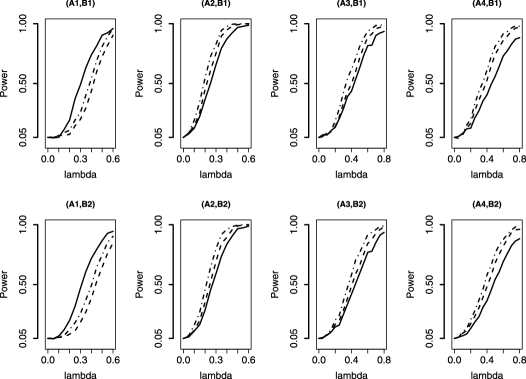
Figure 1: Size-adjusted power curves for $T^{1}_{n}$ (dashed curve) and $T^{2}_{n}$ (dotdash curve) in (17) and $T^{\mathrm{SN}}_{n}$ (solid curve) in (20) as functions of change size $\lambda$ (horizontal axis) with sample size $n=120$ and block length $k_{n}=10$. For (A1, B1)–(A4, B1), the error process $\{e_{i}\}$ is from B1 with $\theta=0.4$; for (A1, B2)–(A4, B2), the error process $\{e_{i}\}$ is from B2 with $\beta=3.0$.

Finally, we point out that the proposed self-normalization-based methods are not robust to models with time-varying correlation structures. For example, consider the model $e_{i}=0.3e_{i-1}+\varepsilon_{i}$ for $1\leq i\leq 60$ and $e_{i}=0.8e_{i-1}+\varepsilon_{i}$ for $61\leq i\leq n$, where $\varepsilon_{i}$ are i.i.d. N(0, 1). With $k_{n}=10$, the sizes (nominal level $5\%$) for the three tests $T^{\mathrm{SN}}_{n}$, $T^{1}_{n}$, $T^{2}_{n}$ are 0.154, 0.196, 0.223 for A1. Future research directions include (i) developing tests for change in the variance or covariance structure for (1) (See Inclán and Tiao [26], Aue et al. [5] and Berkes, Gombay and Horváth [10] for related contributions); and (ii) developing methods that are robust to changes in correlations.

4 Applications to two real data sets

4.1 Annual mean precipitation in Seoul during 1771–2000

The data set consists of annual mean precipitation rates in Seoul during 1771–2000; see Figure 2 for a plot. The mean levels seem to be different for the two time periods 1771–1880 and 1881–2000. Ha and Ha [22] assumed the observations are i.i.d. under the null hypothesis. As shown in Figure 2, the variations change over time. Also, the auto-correlation function plot (not reported here) indicates strong dependence up to lag 18. Therefore, it is more reasonable to apply our self-normalization-based test that is tailored to deal with modulated stationary processes. With sample size $n=230$, by the method in Section 3.1, the optimal block length is about 15. Based on $10^{5}$ bootstrap samples as described in Section 2.4, we obtain the corresponding p-values 0.016, 0.005, 0.045, 0.007, with block length $k_{n}=12,14,16,18$, respectively. For all choices of $k_{n}$, there is compelling evidence that a change point occurred at year 1880. While our result is consistent with that of Ha and Ha [22], our modulated stationary time series framework seems to be more reasonable. Denote by $\mu_{1}$ and $\mu_{2}$ the mean levels over pre-change and post-change time periods 1771–1880 and 1881–2000. For the two sub-periods with sample sizes 110 and 120, the optimal block length is about 12. With $k_{n}=12$, applying the wild bootstrap in Section 2.3 with $10^{5}$ bootstrap samples, we obtain $95\%$ confidence intervals $[121.7,161.3]$ for $\mu_{1}$, $[100.9,114.3]$ for $\mu_{2}$. For the difference $\mu_{1}-\mu_{2}$, with optimal block length $k_{n}=15$, the $95\%$ wild bootstrap confidence interval is $[19.6,48.2]$. Note that the latter confidence interval for $\mu_{1}-\mu_{2}$ does not cover zero, which provides further evidence for $\mu_{1}\neq\mu_{2}$ and the existence of a change point at year 1880.

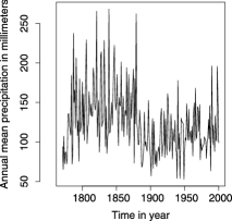
Figure 2: Annual mean precipitation in Seoul from 1771–2000.

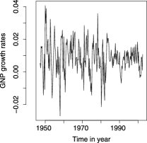
Figure 3: Quarterly U.S. GNP growth rates from 1947–2002.

4.2 Quarterly U.S. GNP growth rates during 1947–2002

The data set consists of quarterly U.S. Gross National Product (GNP) growth rates from the first quarter of 1947 to the third quarter of 2002; see Section 3.8 in Shumway and Stoffer [38] for a stationary autoregressive model approach. However, the plot in Figure 3 suggests a non-stationary pattern: the variation becomes smaller after year 1985 whereas the mean level remains constant. Moreover, the stationarity test in Kwiatkowski et al. [28] provides fairly strong evidence for non-stationarity with a p-value of 0.088. With the block length $k_{n}=12,14,16,18$, we obtain the corresponding p-values $0.853,0.922,0.903,0.782$, and hence there is no evidence to reject the null hypothesis of a constant mean $\mu$. Based on $k_{n}=15$, the $95\%$ wild bootstrap confidence interval for $\mu$ is $[0.66\%,1.00\%]$. To test whether there is a change point in the variance, by the discussion in the last paragraph of Section 2.4, we consider $\tilde{X}_{i}=(X_{i}-\underline{X}_{n})^{2}$. With $k_{n}=12,14,16,18$, the corresponding p-values are $0.001,0.006,0.001,0.010$, indicating strong evidence for a change point in the variance at year 1984. In summary, we conclude that there is no change point in the mean level, but there is a change point in the variance at year 1984.

Appendix: Proofs

Proof of Theorem 2.1 Let $r_{j}=|\sigma_{j}|+\sum^{j}_{i=2}|\sigma_{i}-\sigma_{i-1}|$. By the triangle inequality, we have $r_{j}\leq r_{n}$. Recall $S_{i}$ in (6). By the summation by parts formula, (10) follows via

$$F_{j} = \sum^{j}_{i=1}\sigma_{i}(S_{i}-S_{i-1})=\sigma_{j}S_{j}+\sum^{j-1}_{i=1}(\sigma_{i}-\sigma_{i+1})S_{i}$$

$$= \sigma_{j}\tau B_{j}+\sum^{j-1}_{i=1}(\sigma_{i}-\sigma_{i+1})\tau B_{i}+\mathrm{O}_{\mathrm{a.s.}}(r_{n}\Delta_{n})$$

$$= \tau\sum^{j}_{i=1}\sigma_{i}(B_{i}-B_{i-1})+\mathrm{O}_{\mathrm{a.s.}}(r_{n}\Delta_{n}).$$

By Kolmogorov’s maximal inequality for independent random variables, for $\delta>0$,

$$P\Biggl{\{}\max_{1\leq j\leq n}\Biggl{|}\sum^{j}_{i=1}\sigma_{i}(B_{i}-B_{i-1})\Biggr{|}\geq\delta\Sigma_{n}\Biggr{\}}\leq(\delta\Sigma_{n})^{-2}E\Biggl{[}\Biggl{\{}\sum^{n}_{i=1}\sigma_{i}(B_{i}-B_{i-1})\Biggr{\}}^{2}\Biggr{]}=\delta^{-2}.\quad$$ (32)

Thus, by (Appendix: Proofs), $\max_{1\leq j\leq n}|F_{j}|=\mathrm{O}_{\mathrm{p}}(\Sigma_{n}+r_{n}\Delta_{n})$. Observe that

$$\underline{V}^{2}_{j}-\Sigma^{2}_{j}=W_{j}-F_{j}^{2}/j,\qquad\mbox{where }W_{j}=\sum^{j}_{i=1}\sigma^{2}_{i}(e^{2}_{i}-1).$$ (33)

By (6), the same argument in (Appendix: Proofs) and (32) shows $W_{j}=\mathrm{O}_{\mathrm{p}}(\Sigma^{*2}_{n}+r^{*}_{n}\Delta_{n})$, uniformly. The desired result then follows via (33).

Proof of Theorem 2.2 Denote by $\Phi(x)$ the standard normal distribution function. By Proposition 2.2 and Slutsky’s theorem, $\mathbb{P}(H_{n}/\hat{\tau}\leq x)\to\Phi(x)$ for each fixed $x\in\mathbb{R}$. Since $\Phi(x)$ is a continuous distribution, $\sup_{x\in\mathbb{R}}|\mathbb{P}(H_{n}/\hat{\tau}\leq x)-\Phi(x)|=0$. It remains to prove $\sup_{x\in\mathbb{R}}|\mathbb{P}^{*}(H^{*}_{n}\leq x)-\Phi(x)|\to 0$, in probability. Notice that, conditioning on $\{e_{i}\}$, $\{\xi_{i}\}$ are independent random variables with zero mean. By the Berry–Esséen bound in Bentkus, Bloznelis and Götze [9], there exists a finite constant $c$ such that

$$\sup_{x\in\mathbb{R}}|\mathbb{P}^{*}(H^{*}_{n}\leq x)-\Phi(x)|\leq c\sum^{n}_{i=1}E^{*}(|\xi_{i}|^{3})\Biggl{\{}\sum^{n}_{i=1}E^{*}(|\xi_{i}|^{2})\Biggr{\}}^{-3/2},$$ (34)

where $E^{*}$ denotes conditional expectations given $\{e_{i}\}$. Clearly, $E^{*}(|\xi_{i}|^{2})=\sigma^{2}_{i}e^{2}_{i}E(\alpha^{2}_{1})$ and $E(|\xi_{i}|^{3})=\sigma^{3}_{i}|e^{3}_{i}|E(|\alpha^{3}_{1}|)$. Thus, under the assumption $e_{i}\in\mathcal{L}^{3}$, we have $\sum^{n}_{i=1}E^{*}(|\xi_{i}|^{3})=\mathrm{O}_{\mathrm{p}}(\sum^{n}_{i=1}\sigma^{3}_{i})$. Meanwhile, by the proof of Theorem 2.1, $\sum^{n}_{i=1}E^{*}(|\xi_{i}|^{2})=\sum^{n}_{i=1}\sigma^{2}_{i}e^{2}_{i}=\{1+\mathrm{o}_{\mathrm{p}}(1)\}\sum^{n}_{i=1}\sigma^{2}_{i}$. Therefore, the desired result follows from (34) in view of (15).

Proof of Theorem 2.3 For $cn\leq j\leq(1-c)n$, $c\leq(1-j/n),j/n\leq 1-c$. For $S_{X}(j)$ in (18), by (10), we have $\max_{cn\leq j\leq(1-c)n}|S_{X}(j)-\tau\widetilde{S}_{X}(j)|=\mathrm{O}_{\mathrm{a.s.}}(r_{n}\Delta_{n})$, where

$$\widetilde{S}_{X}(j)=\biggl{(}1-\frac{j}{n}\biggr{)}\sum^{j}_{i=1}\sigma_{i}(B_{i}-B_{i-1})-\frac{j}{n}\sum^{n}_{i=j+1}\sigma_{i}(B_{i}-B_{i-1}).$$

By (11), $\max_{cn\leq j\leq(1-c)n}|(1-j/n)^{2}\underline{V}^{2}_{j}+(j/n)^{2}\overline{V}^{2}_{j}-V^{2}_{j}|=\mathrm{O}_{\mathrm{p}}(\varpi_{n})$, where

$$V^{2}_{j}=(1-j/n)^{2}\sum^{j}_{i=1}\sigma^{2}_{i}+(j/n)^{2}\sum^{n}_{i=j+1}\sigma^{2}_{i}\quad\mbox{and}\quad\varpi_{n}=(r^{2}_{n}\Delta^{2}_{n}+\Sigma^{2}_{n})/n+\Sigma^{*2}_{n}+r^{*}_{n}\Delta_{n}.$$

For $cn\leq j\leq(1-c)n$, $V^{2}_{j}\geq c^{2}\Sigma^{2}_{n}$. Thus, condition (14) implies $\varpi_{n}=\mathrm{o}(V^{2}_{j})$ and $\{V^{2}_{j}+\mathrm{O}_{\mathrm{p}}(\varpi_{n})\}^{1/2}=V_{j}+\mathrm{O}_{\mathrm{p}}(\varpi_{n}/V_{j})$. Therefore, uniformly over $cn\leq j\leq(1-c)n$,

$$T_{n}(j)-\tau\widetilde{T}_{n}(j)=\frac{\tau\widetilde{S}_{X}(j)+\mathrm{O}_{\mathrm{a.s.}}(r_{n}\Delta_{n})}{V_{j}+\mathrm{O}_{\mathrm{p}}(\varpi_{n}/V_{j})}-\frac{\tau\widetilde{S}_{X}(j)}{V_{j}}=\mathrm{O}_{\mathrm{p}}\biggl{\{}\frac{r_{n}\Delta_{n}}{V_{j}}+\frac{\varpi_{n}\widetilde{S}_{X}(j)}{V_{j}^{3}}\biggr{\}}.$$

By (32), $\max_{j}|\widetilde{S}_{X}(j)|=\mathrm{O}_{\mathrm{p}}(\Sigma_{n})$. Thus, the result follows in view of $V_{j}\geq c\Sigma_{n}$.

Proof of Theorem 2.4 Condition $M_{n}\to 0$ implies $\max_{1\leq j\leq\ell_{n}}r(j)\Delta_{n}/\Sigma(j)\to 0$. By (11),

$$\omega_{j}:=\frac{V^{2}(j)}{\Sigma^{2}(j)}-1=\mathrm{O}_{\mathrm{p}}\biggl{\{}\frac{\Sigma^{*2}(j)+r^{*}(j)\Delta_{n}}{\Sigma^{2}(j)}+\frac{1}{k_{n}}\biggr{\}}=\mathrm{O}_{\mathrm{p}}(M_{n})\to 0.$$ (35)

Define $U_{j}=\Sigma^{-1}(j)\sum_{i\in\mathcal{I}_{j}}\sigma_{i}(B_{i}-B_{i-1})$. Clearly, $U_{1},\ldots,U_{\ell_{n}}$ are independent standard normal random variables. Thus, $\max_{1\leq j\leq\ell_{n}}|U_{j}|=\mathrm{O}_{\mathrm{p}}\{\sqrt{\log(\ell_{n})}\}=\mathrm{O}_{\mathrm{p}}\{\sqrt{\log(n)}\}$. By (10), $\underline{X}_{n}-\mu=\mathrm{O}_{\mathrm{p}}\{(\Sigma_{n}+r_{n}\Delta_{n})/n\}=\mathrm{O}_{\mathrm{p}}(\Sigma_{n}/n)$. Recall the definition of $D_{j}$ in (22). By the same argument in (10), using $\sqrt{1+x}=1+\mathrm{O}(x)$ as $x\to 0$, we have

$$D_{j} = \frac{k_{n}\{\bar{X}(j)-\mu\}}{\Sigma(j)}\frac{1}{\sqrt{1+\omega_{j}}}+\frac{k_{n}(\mu-\underline{X}_{n})}{\Sigma(j)}\frac{1}{\sqrt{1+\omega_{j}}}$$

$$= \biggl{[}\tau U_{j}+\mathrm{O}_{\mathrm{a.s.}}\biggl{\{}\frac{r(j)\Delta_{n}}{\Sigma(j)}\biggr{\}}\biggr{]}\{1+\mathrm{O}(\omega_{j})\}+\mathrm{O}_{\mathrm{p}}\biggl{\{}\frac{k_{n}\Sigma_{n}}{n\Sigma(j)}\biggr{\}}$$

$$= \tau U_{j}+\mathrm{O}_{\mathrm{p}}\biggl{\{}\sqrt{\log(n)}M_{n}+\frac{\Sigma_{n}}{\ell_{n}\Sigma(j)}\biggr{\}}.$$

By the latter expression and $\log(n)M_{n}\to 0$, we can easily verify $\hat{\tau}^{2}-\tau^{2}=\mathrm{O}_{\mathrm{p}}(\chi_{n})$.

References

- [1] {barticle}[mr] \bauthor\bsnmAdak, \bfnmSudeshna\binitsS. (\byear1998). \btitleTime-dependent spectral analysis of nonstationary time series. \bjournalJ. Amer. Statist. Assoc. \bvolume93 \bpages1488–1501. \bidissn=0162-1459, mr=1666643 \bptokimsref \endbibitem
- [2] {barticle}[mr] \bauthor\bsnmAltman, \bfnmN. S.\binitsN.S. (\byear1990). \btitleKernel smoothing of data with correlated errors. \bjournalJ. Amer. Statist. Assoc. \bvolume85 \bpages749–759. \bidissn=0162-1459, mr=1138355 \bptokimsref \endbibitem
- [3] {barticle}[mr] \bauthor\bsnmAnděl, \bfnmJiří\binitsJ., \bauthor\bsnmNetuka, \bfnmIvan\binitsI. &\bauthor\bsnmZvźra, \bfnmKarel\binitsK. (\byear1984). \btitleOn threshold autoregressive processes. \bjournalKybernetika (Prague) \bvolume20 \bpages89–106. \bidissn=0023-5954, mr=0747062 \bptokimsref \endbibitem
- [4] {barticle}[mr] \bauthor\bsnmAndrews, \bfnmDonald W. K.\binitsD.W.K. (\byear1993). \btitleTests for parameter instability and structural change with unknown change point. \bjournalEconometrica \bvolume61 \bpages821–856. \biddoi=10.2307/2951764, issn=0012-9682, mr=1231678 \bptokimsref \endbibitem
- [5] {barticle}[mr] \bauthor\bsnmAue, \bfnmAlexander\binitsA., \bauthor\bsnmHörmann, \bfnmSiegfried\binitsS., \bauthor\bsnmHorváth, \bfnmLajos\binitsL. &\bauthor\bsnmReimherr, \bfnmMatthew\binitsM. (\byear2009). \btitleBreak detection in the covariance structure of multivariate time series models. \bjournalAnn. Statist. \bvolume37 \bpages4046–4087. \biddoi=10.1214/09-AOS707, issn=0090-5364, mr=2572452 \bptokimsref \endbibitem
- [6] {barticle}[mr] \bauthor\bsnmAue, \bfnmAlexander\binitsA., \bauthor\bsnmHorváth, \bfnmLajos\binitsL., \bauthor\bsnmHušková, \bfnmMarie\binitsM. &\bauthor\bsnmKokoszka, \bfnmPiotr\binitsP. (\byear2008). \btitleTesting for changes in polynomial regression. \bjournalBernoulli \bvolume14 \bpages637–660. \biddoi=10.3150/08-BEJ122, issn=1350-7265, mr=2537806 \bptokimsref \endbibitem
- [7] {barticle}[mr] \bauthor\bsnmAue, \bfnmAlexander\binitsA., \bauthor\bsnmHorváth, \bfnmLajos\binitsL., \bauthor\bsnmKokoszka, \bfnmPiotr\binitsP. &\bauthor\bsnmSteinebach, \bfnmJosef\binitsJ. (\byear2008). \btitleMonitoring shifts in mean: Asymptotic normality of stopping times. \bjournalTEST \bvolume17 \bpages515–530. \biddoi=10.1007/s11749-006-0041-7, issn=1133-0686, mr=2470096 \bptokimsref \endbibitem
- [8] {barticle}[mr] \bauthor\bsnmBai, \bfnmJushan\binitsJ. &\bauthor\bsnmPerron, \bfnmPierre\binitsP. (\byear1998). \btitleEstimating and testing linear models with multiple structural changes. \bjournalEconometrica \bvolume66 \bpages47–78. \biddoi=10.2307/2998540, issn=0012-9682, mr=1616121 \bptokimsref \endbibitem
- [9] {barticle}[mr] \bauthor\bsnmBentkus, \bfnmV.\binitsV., \bauthor\bsnmBloznelis, \bfnmM.\binitsM. &\bauthor\bsnmGötze, \bfnmF.\binitsF. (\byear1996). \btitleA Berry–Esséen bound for Student’s statistic in the non-i.i.d. case. \bjournalJ. Theoret. Probab. \bvolume9 \bpages765–796. \biddoi=10.1007/BF02214086, issn=0894-9840, mr=1400598 \bptokimsref \endbibitem
- [10] {barticle}[mr] \bauthor\bsnmBerkes, \bfnmIstván\binitsI., \bauthor\bsnmGombay, \bfnmEdit\binitsE. &\bauthor\bsnmHorváth, \bfnmLajos\binitsL. (\byear2009). \btitleTesting for changes in the covariance structure of linear processes. \bjournalJ. Statist. Plann. Inference \bvolume139 \bpages2044–2063. \biddoi=10.1016/j.jspi.2008.09.004, issn=0378-3758, mr=2497559 \bptokimsref \endbibitem
- [11] {bbook}[mr] \bauthor\bsnmBillingsley, \bfnmPatrick\binitsP. (\byear1968). \btitleConvergence of Probability Measures. \baddressNew York: \bpublisherWiley. \bidmr=0233396 \bptokimsref \endbibitem
- [12] {barticle}[mr] \bauthor\bsnmBühlmann, \bfnmPeter\binitsP. (\byear2002). \btitleBootstraps for time series. \bjournalStatist. Sci. \bvolume17 \bpages52–72. \biddoi=10.1214/ss/1023798998, issn=0883-4237, mr=1910074 \bptokimsref \endbibitem
- [13] {barticle}[mr] \bauthor\bsnmCarlstein, \bfnmEdward\binitsE. (\byear1986). \btitleThe use of subseries values for estimating the variance of a general statistic from a stationary sequence. \bjournalAnn. Statist. \bvolume14 \bpages1171–1179. \biddoi=10.1214/aos/1176350057, issn=0090-5364, mr=0856813 \bptokimsref \endbibitem
- [14] {bbook}[mr] \bauthor\bsnmCsörgő, \bfnmMiklós\binitsM. &\bauthor\bsnmHorváth, \bfnmLajos\binitsL. (\byear1997). \btitleLimit Theorems in Change-Point Analysis. \bseriesWiley Series in Probability and Statistics. \baddressChichester: \bpublisherWiley. \bidmr=2743035 \bptokimsref \endbibitem
- [15] {barticle}[mr] \bauthor\bsnmDahlhaus, \bfnmR.\binitsR. (\byear1997). \btitleFitting time series models to nonstationary processes. \bjournalAnn. Statist. \bvolume25 \bpages1–37. \biddoi=10.1214/aos/1034276620, issn=0090-5364, mr=1429916 \bptokimsref \endbibitem
- [16] {barticle}[mr] \bauthor\bsnmDahlhaus, \bfnmRainer\binitsR. &\bauthor\bsnmPolonik, \bfnmWolfgang\binitsW. (\byear2009). \btitleEmpirical spectral processes for locally stationary time series. \bjournalBernoulli \bvolume15 \bpages1–39. \biddoi=10.3150/08-BEJ137, issn=1350-7265, mr=2546797 \bptokimsref \endbibitem
- [17] {barticle}[mr] \bauthor\bsnmDavidson, \bfnmRussell\binitsR. &\bauthor\bsnmFlachaire, \bfnmEmmanuel\binitsE. (\byear2008). \btitleThe wild bootstrap, tamed at last. \bjournalJ. Econometrics \bvolume146 \bpages162–169. \biddoi=10.1016/j.jeconom.2008.08.003, issn=0304-4076, mr=2459651 \bptokimsref \endbibitem
- [18] {barticle}[mr] \bauthor\bparticlede \bsnmJong, \bfnmRobert M.\binitsR.M. &\bauthor\bsnmDavidson, \bfnmJames\binitsJ. (\byear2000). \btitleConsistency of kernel estimators of heteroscedastic and autocorrelated covariance matrices. \bjournalEconometrica \bvolume68 \bpages407–423. \biddoi=10.1111/1468-0262.00115, issn=0012-9682, mr=1748008 \bptokimsref \endbibitem
- [19] {barticle}[mr] \bauthor\bsnmEfron, \bfnmB.\binitsB. (\byear1979). \btitleBootstrap methods: Another look at the jackknife. \bjournalAnn. Statist. \bvolume7 \bpages1–26. \bidissn=0090-5364, mr=0515681 \bptokimsref \endbibitem
- [20] {bbook}[mr] \bauthor\bsnmFan, \bfnmJianqing\binitsJ. &\bauthor\bsnmYao, \bfnmQiwei\binitsQ. (\byear2003). \btitleNonlinear Time Series: Nonparametric and Parametric Methods. \bseriesSpringer Series in Statistics. \baddressNew York: \bpublisherSpringer. \biddoi=10.1007/b97702, mr=1964455 \bptokimsref \endbibitem
- [21] {barticle}[mr] \bauthor\bsnmGötze, \bfnmF.\binitsF. &\bauthor\bsnmKünsch, \bfnmH. R.\binitsH.R. (\byear1996). \btitleSecond-order correctness of the blockwise bootstrap for stationary observations. \bjournalAnn. Statist. \bvolume24 \bpages1914–1933. \biddoi=10.1214/aos/1069362303, issn=0090-5364, mr=1421154 \bptokimsref \endbibitem
- [22] {barticle}[auto:STB—2011/12/23—09:17:17] \bauthor\bsnmHa, \bfnmK. J.\binitsK.J. &\bauthor\bsnmHa, \bfnmE.\binitsE. (\byear2006). \btitleClimatic change and interannual fluctuations in the long-term record of monthly precipitation for Seoul. \bjournalInt. J. Climatol. \bvolume26 \bpages607–618. \bptokimsref \endbibitem
- [23] {barticle}[mr] \bauthor\bsnmHansen, \bfnmBruce E.\binitsB.E. (\byear1995). \btitleRegression with nonstationary volatility. \bjournalEconometrica \bvolume63 \bpages1113–1132. \biddoi=10.2307/2171723, issn=0012-9682, mr=1348515 \bptokimsref \endbibitem
- [24] {barticle}[mr] \bauthor\bsnmHansen, \bfnmBruce E.\binitsB.E. (\byear2000). \btitleTesting for structural change in conditional models. \bjournalJ. Econometrics \bvolume97 \bpages93–115. \biddoi=10.1016/S0304-4076(99)00068-8, issn=0304-4076, mr=1788819 \bptokimsref \endbibitem
- [25] {barticle}[mr] \bauthor\bsnmHorváth, \bfnmLajos\binitsL. (\byear1993). \btitleThe maximum likelihood method for testing changes in the parameters of normal observations. \bjournalAnn. Statist. \bvolume21 \bpages671–680. \biddoi=10.1214/aos/1176349143, issn=0090-5364, mr=1232511 \bptokimsref \endbibitem
- [26] {barticle}[mr] \bauthor\bsnmInclán, \bfnmCarla\binitsC. &\bauthor\bsnmTiao, \bfnmGeorge C.\binitsG.C. (\byear1994). \btitleUse of cumulative sums of squares for retrospective detection of changes of variance. \bjournalJ. Amer. Statist. Assoc. \bvolume89 \bpages913–923. \bidissn=0162-1459, mr=1294735 \bptokimsref \endbibitem
- [27] {barticle}[mr] \bauthor\bsnmKünsch, \bfnmHans R.\binitsH.R. (\byear1989). \btitleThe jackknife and the bootstrap for general stationary observations. \bjournalAnn. Statist. \bvolume17 \bpages1217–1241. \biddoi=10.1214/aos/1176347265, issn=0090-5364, mr=1015147 \bptokimsref \endbibitem
- [28] {barticle}[auto:STB—2011/12/23—09:17:17] \bauthor\bsnmKwiatkowski, \bfnmD.\binitsD., \bauthor\bsnmPhillips, \bfnmP. C. B.\binitsP.C.B., \bauthor\bsnmSchmidt, \bfnmP.\binitsP. &\bauthor\bsnmShin, \bfnmY.\binitsY. (\byear1992). \btitleTesting the null hypothesis of stationarity against the alternative of a unit root. \bjournalJ. Econometrics \bvolume54 \bpages159–178. \bptokimsref \endbibitem
- [29] {bbook}[mr] \bauthor\bsnmLahiri, \bfnmS. N.\binitsS.N. (\byear2003). \btitleResampling Methods for Dependent Data. \bseriesSpringer Series in Statistics. \baddressNew York: \bpublisherSpringer. \bidmr=2001447 \bptokimsref \endbibitem
- [30] {barticle}[mr] \bauthor\bsnmLiu, \bfnmRegina Y.\binitsR.Y. (\byear1988). \btitleBootstrap procedures under some non-i.i.d. models. \bjournalAnn. Statist. \bvolume16 \bpages1696–1708. \biddoi=10.1214/aos/1176351062, issn=0090-5364, mr=0964947 \bptokimsref \endbibitem
- [31] {barticle}[mr] \bauthor\bsnmMüller, \bfnmUlrich K.\binitsU.K. (\byear2007). \btitleA theory of robust long-run variance estimation. \bjournalJ. Econometrics \bvolume141 \bpages1331–1352. \biddoi=10.1016/j.jeconom.2007.01.019, issn=0304-4076, mr=2413504 \bptokimsref \endbibitem
- [32] {barticle}[mr] \bauthor\bsnmPettitt, \bfnmA. N.\binitsA.N. (\byear1980). \btitleA simple cumulative sum type statistic for the change-point problem with zero–one observations. \bjournalBiometrika \bvolume67 \bpages79–84. \biddoi=10.1093/biomet/67.1.79, issn=0006-3444, mr=0570508 \bptokimsref \endbibitem
- [33] {barticle}[mr] \bauthor\bsnmPhillips, \bfnmPeter C. B.\binitsP.C.B., \bauthor\bsnmSun, \bfnmYixiao\binitsY. &\bauthor\bsnmJin, \bfnmSainan\binitsS. (\byear2007). \btitleLong run variance estimation and robust regression testing using sharp origin kernels with no truncation. \bjournalJ. Statist. Plann. Inference \bvolume137 \bpages985–1023. \biddoi=10.1016/j.jspi.2006.06.033, issn=0378-3758, mr=2301731 \bptokimsref \endbibitem
- [34] {barticle}[mr] \bauthor\bsnmPolitis, \bfnmDimitris N.\binitsD.N. &\bauthor\bsnmRomano, \bfnmJoseph P.\binitsJ.P. (\byear1994). \btitleLarge sample confidence regions based on subsamples under minimal assumptions. \bjournalAnn. Statist. \bvolume22 \bpages2031–2050. \biddoi=10.1214/aos/1176325770, issn=0090-5364, mr=1329181 \bptokimsref \endbibitem
- [35] {barticle}[mr] \bauthor\bsnmRobbins, \bfnmMichael W.\binitsM.W., \bauthor\bsnmLund, \bfnmRobert B.\binitsR.B., \bauthor\bsnmGallagher, \bfnmColin M.\binitsC.M. &\bauthor\bsnmLu, \bfnmQiQi\binitsQ. (\byear2011). \btitleChangepoints in the North Atlantic tropical cyclone record. \bjournalJ. Amer. Statist. Assoc. \bvolume106 \bpages89–99. \biddoi=10.1198/jasa.2011.ap10023, issn=0162-1459, mr=2816704 \bptokimsref \endbibitem
- [36] {barticle}[mr] \bauthor\bsnmShao, \bfnmQi Man\binitsQ.M. (\byear1993). \btitleAlmost sure invariance principles for mixing sequences of random variables. \bjournalStochastic Process. Appl. \bvolume48 \bpages319–334. \biddoi=10.1016/0304-4149(93)90051-5, issn=0304-4149, mr=1244549 \bptokimsref \endbibitem
- [37] {barticle}[mr] \bauthor\bsnmShao, \bfnmXiaofeng\binitsX. &\bauthor\bsnmZhang, \bfnmXianyang\binitsX. (\byear2010). \btitleTesting for change points in time series. \bjournalJ. Amer. Statist. Assoc. \bvolume105 \bpages1228–1240. \biddoi=10.1198/jasa.2010.tm10103, issn=0162-1459, mr=2752617 \bptokimsref \endbibitem
- [38] {bbook}[mr] \bauthor\bsnmShumway, \bfnmRobert H.\binitsR.H. &\bauthor\bsnmStoffer, \bfnmDavid S.\binitsD.S. (\byear2006). \btitleTime Series Analysis and Its Applications: With R Examples, \bedition2nd ed. \bseriesSpringer Texts in Statistics. \baddressNew York: \bpublisherSpringer. \bidmr=2228626 \bptokimsref \endbibitem
- [39] {barticle}[mr] \bauthor\bsnmWu, \bfnmC. F. J.\binitsC.F.J. (\byear1986). \btitleJackknife, bootstrap and other resampling methods in regression analysis. \bjournalAnn. Statist. \bvolume14 \bpages1261–1295. \biddoi=10.1214/aos/1176350142, issn=0090-5364, mr=0868303 \bptnotecheck related \bptokimsref \endbibitem
- [40] {barticle}[mr] \bauthor\bsnmWu, \bfnmWei Biao\binitsW.B. (\byear2007). \btitleStrong invariance principles for dependent random variables. \bjournalAnn. Probab. \bvolume35 \bpages2294–2320. \biddoi=10.1214/009117907000000060, issn=0091-1798, mr=2353389 \bptokimsref \endbibitem
- [41] {barticle}[auto:STB—2011/12/23—09:17:17] \bauthor\bsnmZhao, \bfnmZ.\binitsZ. (\byear2011). \btitleA self-normalized confidence interval for the mean of a class of non-stationary processes. \bjournalBiometrika \bvolume98 \bpages81–90. \bptokimsref \endbibitem