Real-Time Phase Masks for Interactive Stimulation of Optogenetic Neurons

Abstract

Experiments with networks of optogenetically altered neurons require stimulation with high spatio-temporal selectivity. Computer-assisted holography is an energy-efficient method for robust and reliable addressing of single neurons on the millisecond-timescale inherent to biologial information processing. We show that real-time control of neurons can be achieved by a CUDA-based hologram computation.

I Introduction

The development of light-sensitive neurons has been a milestone in optogenetics Deisseroth2006 . The ability to engineer a neuron’s optical sensitivity by genetic manipulation is crucial for a non-destructive and fast, yet accurate photostimulation (PS) of individual sites in networks of living neurons. In vivo interaction with individual neurons is fundamental for a concise experimental study of such basic neurological processes like the mechanisms of learning. In terms of energy efficiency and spatial resolution holographic methods are considered to be the most suitable for PS Golan2009a .

Holograms, i.e. computer generated phase masks (PM), displayed on a spatial light modulator (SLM) realize pixel-wise phase retardations of a coherent laser beam. Upon illumination the intensity of the Fourier transform of the PM yields a high-resolution optical stimulation pattern (OSP) at the specimen. For a sketch of the experimental setup see Fig. 1. The OSP follows from the subset of neurons selected for stimulation. By targeting specific neurons the neural activity in the network and thus its collective behavior can be influenced.

The basis of neural activity is the generation of spikes in the membrane potential at the axon hillock due to synaptic input. The spikes travel along the axon to the synaptic connections to other nerve cells. In genetically altered neurons light-sensitive ion channels are expressed in the cell membrane. If lit with the correct frequency the ion channels open and thus change the membrane potential. This either inhibits or enhances spike generation. After transmission to the next neuron the spike adds to the synaptic input which may lead to another spike.

For interactive modification of the spiking behavior the optical stimulus must be generated within the time a spike needs to travel from one neuron to another. Interspike intervals of adjacent neurons are in the range of 10-20 ms and set the time-scale for computing the unknown PM. Due to this severe time constraint multi-site stimulation thus had to use precomputed PMs, up to now. For interactive network control PMs must be computed online which for frame rates in the required range of 0.1 to 1 kHz poses a substantial challenge. On current many- and multi-core processing units this requires extensive parallelization.

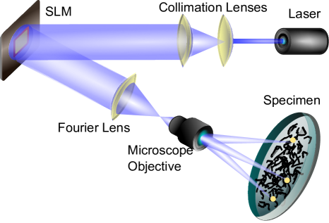
Figure 1: Holographic illumination of a network of optogenetically altered neurons.

Mathematically, computing a PM for a given OSP constitutes an inverse problem equivalent to wavefront reconstruction (see Luke2002 and references therein) and is an instance of the phase retrieval problem (PRP) in diffraction imaging Rayleigh92 . Numerical approaches to the phase problem abound, but convergence results and global solutions are limited to special cases Hauptman ; BCL1 that do not necessarily apply to the case discussed in this paper. An arbitrary OSP is unlikely to have a phase-only Fourier transform. Thus our PRP is fundamentally inconsistent as defined in Luke11 . To account for the mathematical structure, a careful analysis of the performance of the parallelization techniques available and a strong focus on long-term software reusability distinguishes this work from others, e.g. Masuda:06 ; Shimobaba:10 ; Weng:12 . Useful approximations of a PM for a given OSP can be achieved by iterative algorithms like the widely used Method of Alternating Projections Neumann50 , also known as Gerchberg-Saxton algorithm Gerchberg1972 .

In this work we will combine parallel computation on graphics cards with C++-based generic programming and a sound mathematical theory. Only this combination of techniques allows to generate phase masks within less than 10 ms, matching the dynamics of neural activity.

II Method of Alternating Projections

The wavefront is to be altered by a phase shift at the finite number of pixels of the SLM. The entire system is modeled on a finite dimensional vector space. Let $L_{x},L_{y}>0$ be the dimensions of the SLM and $n_{x},n_{y}$ the respective number of pixels. We seek a signal $u\in\mathbb{C}^{N}$ for $N\equiv n_{x}\times n_{y}$. The intensity distribution of the laser beam sets the amplitude of the wavefront $u$ on the SLM. Assuming a constant intensity over one pixel, we discretize the intensity distribution by the nonnegative $p\in\mathbb{R}^{N}$. Wavefronts $u$ emanating from the SLM are given by the set of vectors

$$S \equiv \{u\in\mathbb{C}^{N}~{}:~{}|u_{jk}|=p_{jk},$$ (1)

$$\quad j=1,2,\dots,n_{x},~{}k=1,2,\dots,n_{y}\}.$$

Propagation of the light through the lens system is modeled by Fraunhofer diffraction Goodman . The light at the SLM is related to the observed OSP at the specimen by the Fourier transform $F$. Waves with modulus matching the amplitude distribution $m\in\mathbb{R}^{N}$ of the OSP form the set

$$M\equiv\{u\in\mathbb{C}^{N}~{}:~{}|(Fu)_{jk}|=m_{jk},\quad j\leq n_{x},~{}k\leq n_{y}\}.$$ (2)

On the one hand our wavefront must fulfill the amplitude constraint Eq. (1), on the other hand the amplitudes of its Fourier transform are fixed by the intensity distribution of the stimulation pattern, Eq. (2). Altogether, the mathematical problem we address is to

$$\mbox{Find}~{}u\in S\cap M.$$ (3)

For a nonempty intersection the problem is defined to be consistent; otherwise inconsistent or ill-posed. A common algorithm for problems of this type is the method of alternating projections Neumann50 ; Gerchberg1972 . For a review of this and other projection-based approaches for the PRP see BCL1 . Algorithms of this kind are built on projection operators onto the constraint sets $S$ and $M$. By a projection of a point $u$ in a space $X$ onto a subset $C$ of that space, we mean the mapping of that point to the set of nearest points in $C$ with respect to the norm induced by the real inner product on $X$. For general PRPs, it was proved in Luke2002 that

$$P_{S}u = \left\{v\,:\,v_{jk}=\begin{cases}p_{jk}\frac{u_{jk}}{|u_{jk}|},&\text{if $u_{jk}\neq 0$;}\\ p_{jk}\exp(i\theta),&\mbox{for }\theta\in[0,2\pi)\end{cases}\right\},\hskip 19.91684pt$$ (4a)

$$P_{M}u = \left\{F^{-1}\widehat{u}~{}:~{}\widehat{u}\in\widehat{M}(u)\right\}$$ (4b)

are projections onto the sets $$S M$$ and , respectively, where

$$\widehat{M}(u)\equiv\left\{\hat{v}~{}:~{}\hat{v}_{jk}=\begin{cases}m_{jk}\frac{(Fu)_{jk}}{|(Fu)_{jk}|},&\text{if }(Fu)_{jk}\neq 0\\ m_{jk}\exp(i\theta),&\mbox{for }\theta\in[0,2\pi)\end{cases}\right\}.$$ (4c)

For given $u^{0}\in\mathbb{C}^{N}$ the method of alternating projections computes the iterates $u^{\nu}$ via

$$u^{\nu+1}\in P_{S}P_{M}u^{\nu},\quad\nu=0,1,2,\dots$$ (5)

The multi-valuedness of Eq. (4) makes Eq. (3) a non-convex feasibility problem Luke2002 . Hence Eq. (5) must be understood as a selection from set-valued mappings. Due to nonconvexity, except in special cases Hauptman , global convergence of Eq. (5) cannot be guaranteed in general. For consistent PRPs local convergence results are available Luke11 . Yet, it is more the exception than the rule that our PRP will be consistent: a set of fixed amplitudes cannot produce an arbitrary OSP. Our numerical experiments indicate that our PRPs are indeed inconsistent as measured by the magnitude of the gap

$$G \equiv \|P_{S}u^{\nu}-P_{M}u^{\nu}\|_{2}$$ (6)

between accumulation points in $M$ and their projections onto $S$. The gap is measured in the standard Euclidean norm $\|\cdot\|_{2}$. This systematic inconsistency is a major difference between optogenetic PS and PRPs due to imaging experiments. In the latter the diffraction pattern comprising the set $M$ is causal, that is, comes from diffraction by a physical object, e.g. a protein crystal. Assuming that Eq. (3) is inconsistent, we content ourselves with finding best approximation pairs $(u^{*},v^{*})\in\mathbb{C}^{N}\times\mathbb{C}^{N}$ with $u^{*}\in S$, $v^{*}\in M$, $P_{M}u^{*}=v^{*}$ and $P_{S}v^{*}=u^{*}$.

To account for the particularities of optogenetic PS, we define the physical error as the sum of the pixel-wise relative violation of deviation tolerances between target and reconstructed OSP HeckesError . We allow for a relative deviation $t_{\ell}=0.1$ for non-zero target pixels and an absolute deviation of $t_{\text{d}}=3\cdot 10^{-4}$ for non-lit pixels. Violations are summed in multiples of $t_{\ell}$ and $t_{d}$. With $u_{jk}^{\nu}$ being the intensity from the current iteration step, $m_{jk}$ the intensity in the target OSP and $\Theta(\cdot)$ the Heaviside step function, the total error is the sum of

$$E_{\ell}^{\nu} = \sum\limits_{pixels\in lit}\left(\frac{t_{\text{d}}|m_{jk}-u_{jk}^{\nu}|}{t_{\ell}m_{jk}}-t_{\text{d}}\right)$$ (7a)

$$\times\Theta\left(\frac{|m_{jk}-u_{jk}^{\nu}|}{m_{jk}}-t_{\ell}\right),\quad~{}~{}$$

$$E_{\text{d}}^{\nu} = \sum\limits_{pixels\in dark}\left(u_{jk}^{\nu}-t_{\text{d}}\right)\cdot\Theta\left(u_{jk}^{\nu}-t_{\text{d}}\right)\,.$$ (7b)

III Unified Implementation

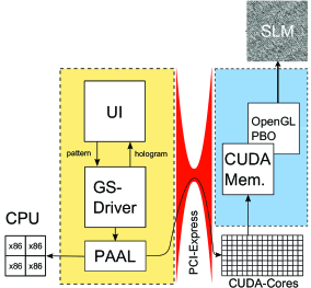
(a)

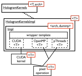
(b)

Figure 2: Left: Software structure and its association with the different hardware components. Right: Class diagram of the PAAL concept. Class names are underlined. Template arguments are given in red boxes. Dashed boxes indicate partial template specializations.

The compound system of CPU and GPU, each with dedicated memories, represents a non-uniform memory access architecture with a very heterogeneous distribution of processing capabilities and internal transfer rates. Figure 2a sketches the class structure and its distribution over the compound system of CPU and GPU. The major bottleneck is the PCIe-BUS. According to the PCIe v2.0 specification it has a maximal transfer rate of 8 GByte/sec although in practice one rather gets 4 to 5 GByte/sec. This will rise to 16 GByte/sec with the forthcoming PCIe v3.0, yet memory transfer rates within the GPU are of the order of 100 GByte/sec. On CPUs with integrated memory controllers the transfer rates are in the range of 20 to 30 GByte/sec. To anticipate the rapid evolution of hardware and parallelization techniques we spent considerable effort on modularizing the program using C++’s templating capabilities. CUDA extends $C$ for programming NVidia GPUs. OpenMP provides multithreaded parallelization on multi-core CPUs. Depending on the parallelization technique the program works on different sides of the PCIe-BUS. To separate hardware-specific optimizations at the low-level, e.g. the details of Eq. (4), from the implementation of algorithms we introduced the concept of a parallel architecture abstraction layer (PAAL). Since most of our computational tasks are data-parallel they are perfect candidates for abstraction with respect to floating-point precision and parallelization. This is achieved by a suitable set of template parameters leaving the generation of the hardware-specific part of the code to the compiler. As FFTs in the projector onto the constraint representing the OSP, Eq. (4b), we use either NVidia’s cuFFT or the FFTW Frigo2005 which offers an OpenMP- as well as a pthreads-based variant.

The aim of the PAAL concept is a quick recombination of algorithms and parallelization strategies by explicit template specializations. The front end comprises the user-interface (UI) and manages the execution of the phase retrieval algorithms for which separate driver classes exist, e.g. GS-DRIVER for the method of alternating projections. The final PM is transferred to an OpenGL framebuffer object for display on the SLM, cf. Fig. 2a.

The PAAL concept is explained best by walking through the essential parts of its class structure. This is done roughly in a top down approach, i.e. from host to device and how things build on each other. A sketch of the class structure is given in Fig. 2b. At the top is the interface to the GS-Driver which is formed by the class HologramKernels. It takes two template arguments: T for the precision and arch for the architecture the algorithm is to run on. At the bottom of the hierarchy is the operation one has to do on a particular pixel.

To express that the class HologramKernels is implemented with HologramKernelsImpl inheritance is private meyers2005effective (indicted by the dashed line in Fig. 2b). The class HologramKernels needs partial specializations for the different architectures because for the CUDA kernels the wrapper functions behave differently with respect to the architecture. On a NVidia GPU they have to call a CUDA kernel. On a CPU they have to either use OpenMP or pthreads for parallelization. The parallel execution of the per-pixel operation via OpenMP or pthreads can be done directly in the specialization of the wrapper function. In the following we omit the pthreads specialization as it is structurally very similar to OpenMP. The wrapper functions are implemented by the internal class Impl of HologramKernelsImpl. The reason for this particular design is that the $C$++ standard does not allow to define partial specializations of (a subset of) the member functions of a class. This issue can be circumvented by introducing an internal class with a dummy template parameter and to partially specialize its members. Within the class Impl the particular type of real and complex numbers is deduced from the template parameter T by means of a suitable Traits structure. This is a typical example of template metaprogramming AbrahamsGurtovoy2004 .

The back end, i.e. the details of the implementation, are stored in a separate source file to keep g++ away from CUDA-specific code. Within the evaluation of Eqs. (4a) and (4c) we need precision-dependent tolerances for what is considered as zero. To this end we localize the inevitable magic numbers in a structure __eps and a function __is_zero. In case of being compiled into a CUDA kernel the __device__ keyword is put into effect indicating that the function can only be executed on the device, i.e. the GPU. Prepending __device__ by __host__ signals the compiler (i.e. nvcc) to compile two versions of a function or operator. One for the execution on the GPU and one for the CPU. At the binary level these are distinct functions.

The actual per-pixel operation is done by an architecture-independent function __ps_element. Its arguments are a pointer d_devPtr* to the beginning of the array of pixels of the iterated image $Fu^{\nu}$, a pointer d_original* to the beginning of the array of pixels of the original image and the lexicographic index of the pixel x. The CUDA kernel __ps (listing 1) basically has the same arguments as the element function. The kernel gets the size of the image as additional argument in order to avoid operating on non-existent pixels. The kernel computes the position x of its pixel from its threadIdx and BlockIdx. Given the pixel position is within the bounds of the array the element function is invoked.

Listing 1: PAAL: CUDA kernel for amplitude adaption

⬇

1template <typename T>

__global__ void __ps(T *d_devPtr, const T *d_original, const int size)

{

int x = blockDim.x*blockIdx.x + threadIdx.x;

if(x < size)

__ps_element<T, gpu_cuda>(d_devPtr, d_original, x);

}

The missing link between back end and driver class is the specializations of the wrapper functions for the kernels. The GPU version (listing 2) starts as many threads as there are pixels for the kernel __ps. Each thread starts the device function __ps_element, so that each pixel (vector element) is processed.

Listing 2: PAAL: GPU specialization of wrapper function

⬇

1template<typename T>

template< typename dummy>

void

HologramKernelsImpl<T>::Impl<gpu_cuda, dummy>::ps

(Complex *d_devPtr, const Complex *d_original, const int size)

{

int threads_per_block = 512;

int blocks = (size + threads_per_block - 1) / threads_per_block;

__ps<T><<<blocks, threads_per_block>>>(d_devPtr, d_original, size);

cudaThreadSynchronize();

}

The CPU-OpenMP version (listing 3) has a  for-loop over all pixels in the image which is parallelized by an OpenMP preprocessor directive. By declaring the __ps_element to be a __host__ __device__ function, we can call the same function from the CPU as from the GPU but without the intermediate kernel layer. In this way we have the actual computation implemented only once. With the individual specialized classes wrapped around this implementation we can choose our computing precision and hardware.

Listing 3: PAAL: CPU specialization of wrapper function

⬇

1template<typename T>

template< typename dummy>

void

HologramKernelsImpl<T>::Impl<cpu, dummy>::ps

(Complex *d_devPtr, const Complex *d_original, const int size)

{

#pragma omp parallel for private(i)

for(int i = 0; i < size; i++)

__ps_element<T, cpu>(d_devPtr, d_original, i);

}

Finally, we have to provide full template specializations of all the combinations of precision and architecture template parameters we want to work with. This must be at the end of the hardware-specific source file as all functions have to be declared and their bodies defined before the class can be explicitly instantiated by the compiler VandervordeJosuttis2002 . The explicit specializations are necessary since we compile the back end with a different compiler than the front end of the program.

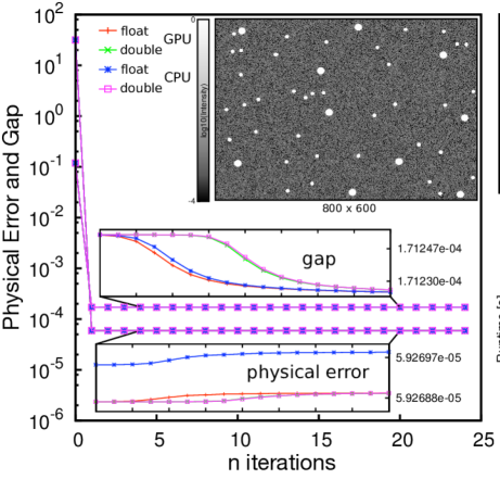
Figure 3: Convergence for a spot pattern of the physical error and the constraint gap.

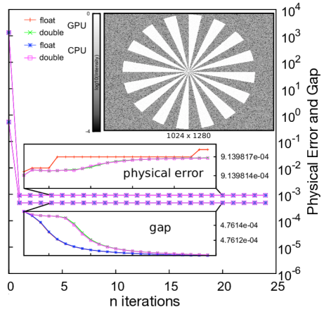
Figure 4: Siemens star: Convergence for single and double precision.

IV Results

The OSP for benchmarking the computation of the phase masks for photo-stimulation are bright spots on a dark background (Fig. 3). The limits of spatial resolution in the reconstruction is tested on the Siemens star (Fig. 4). In both cases we use $P_{M}\hat{u}^{0}$ as initial PM where $u^{0}$ is the 1-bit target OSP. Thus, our initial condition is computed by taking the Fourier transform of the OSP, adapting the Fourier coefficients to the amplitude constraints on the SLM and transforming back into real space again. The other obvious choice as initial condition would be to use random phases. The resulting phase masks do not differ significantly from those obtained by using $P_{M}\hat{u}^{0}$ but take longer to converge. Therefore we skip them in the following discussion.

IV.1 Benchmarking

For interactive holographic PS the physical error, Eq. (7), must reach a sub-threshold level within interspike intervals, i.e. 10 to 20 ms. Hence, the first issue is which parallelization technique provides sufficient performance to meet this requirement. The GPU-based computations were done on a Tesla C2070. The CPU-based ones using OpenMP or pthreads were run on a two-socket system with X5650 Xeons. The CPUs have six cores each. Therefore we decided to use 12 threads, i.e. as much as there are physical cores.

Computing a single PM on the CPU takes several seconds no matter whether OpenMP or pthreads are used. When using CUDA and thus the GPU the total runtimes match the interspike interval constraint. For a typical resolution of $800\times 600$ for an SLM the computation of 25 iterations in single precision takes 45 ms including transfer of the given OSP to the GPU (1 ms). The iteration essentially converges after one step (Fig. 3). Hence a reasonable OSP is available already after much less than 10 ms. However, the precise figure depends on the problem size and number of iteration steps. Thus we keep 10 ms as a conservative bound. The left panel of Fig. 5 shows GPU runtimes per iteration in total and broken down into the contributions due to FFT (green and cyan bars) and enforcement of amplitude constraints (blue and grey bars) for different image sizes and 25 iterations of Eq. (5). The runtimes are further subdivided into the results for single and double precision indicated by the red and magenta bars. The proportion of work to be done in the FFT increases with problem size as the FFT is of log-linear complexity. Enforcing the amplitude constraints is linear in the problem size as each pixel is visited only once per iteration and exchange of information between different pixels is not required.

The right panel of Fig. 5 shows the speedups of the CUDA implementation over its OpenMP and pthreads counterparts. On average CUDA is 50 times faster per iteration than the 12-thread CPU variants. The performance gain per iteration solely depends on the size of an OSP. For the Fermi architecture used in the Tesla C2070 the floating point performance in double precision is half of the one for single precision. This is due to the fact that a double is twice as large as a float and thus requires twice as much memory bandwidth. On CPUs this is less of an issue since they focus on hiding memory latencies by branch prediction. This is reflected by the fact that for double precision the speedup is roughly only half of the one for single precision. Yet, this suffices to get OSPs in double precision within the limits set by the interspike intervals.

(a)

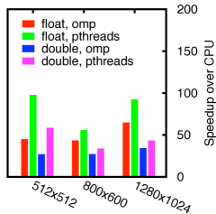
(b)

Figure 5: Left: GPU runtimes per iteration for various image sizes and 25 iterations of Eq. (5). Right: Speedup per iteration for various image sizes.

IV.2 Precision and Convergence

The second issue is the influence of the floating point precision $\epsilon$ on convergence and performance. Figure 3 shows the convergence and reconstruction results for a spot pattern as it would be used in a PS experiment. Figure 4 summarizes the results for the Siemens star which is a standard test image for the spatial resolution achieved by reconstruction algorithms.

The reconstructed OSPs are given as inset with a logarithmic gray scale for intensity. The convergence curves represent the behavior of the physical error, Eq. (7), and the gap, Eq. (6), with respect to the number of iterated steps in Eq. (5). We are interested in the influence of the hardware architecture and the precision. Hence the convergence history is given for single and double precision on GPU and CPU. The details of the curves for the gap and for the physical error in the insets reveal that the behavior primarily depends on whether the computation is run in single or double precision but not on the architecture. This is a subtle effect on the order of the single precision accuracy as illustrated by the scaling of the ordinates in the insets. Both figures show that convergence of the PM in single is as good as in double precision as each quantity has a unique limit value independent of the precision.

The intensity plots of the reconstructed OSPs indicate that the contrast between lit and unlit areas is 3 orders of magnitude. A look at the center of the Siemens star shows that structures down to a few pixels can be resolved. The insets of figures 3 and 4 demonstrate that the gap, as defined in Eq. (6), and the physically motivated error, Eq. (7), saturate within one iteration indicating the inconsistency of our PRP. All further changes are ${\cal O}(\epsilon)$. Convergence does not depend on hardware as the limit values of error and gap are several orders of magnitude larger than any precision. Depending on $\epsilon$ we expect the following resolution limits for $G$.

Our number of pixels is of the order of $10^{6}$. Assuming statistical independence for the errors of $u^{\nu}_{jk}$ we get as theoretical limit $G_{th}\propto 10^{3}\epsilon$, i.e. $10^{-5}$ for single precision ($\epsilon=10^{-8}$) and $10^{-13}$ for double precision ($\epsilon=10^{-16}$). An interesting phenomenon reflecting the difference between exact and finite precision arithmetic is revealed by comparing the convergence behavior as function of $\epsilon$. Single precision (blue and red curves) cannot resolve the inconsistency of the PRP, i.e. whether or not $S\cap M=\emptyset$, as $G\approx G_{th}$. According to Luke11 this should improve convergence. The downside is, that while the PRP appears to be consistent from a numerical point of view, larger $\epsilon$ means worse approximation of the projection operators. For double precision (green and magenta curves) we get more accurate projection operators but at the same time the gap is resolved as for both precisions $G$ is of similar magnitude. This renders the PRP inconsistent again, justifying our assumption of inconsistency. Our results also show that, despite a rather large $G$ the method of alternating projections does not suffer from stagnation at bad local minima which otherwise would call for more sophisticated algorithms like RAAR Luke2005 .

V Conclusions

Mathematically, computing a phase-only hologram to create an OSP which selects predetermined neurons is equivalent to the problem of wavefront reconstruction. Useful approximations of a PM for a given OSP can only be achieved by iterative algorithms like the widely used Method of Alternating Projections.

From the point of view of software engineering we have shown how to integrate CUDA into a complex software environment in a modular way without sacrificing performance. The high modularity of our simulation framework has several key advantages. Code redundancy is minimized. The template techniques let the code reflect the mathematical structure of the problem. The effort to switch between the three parallelization techniques tested, CUDA, OpenMP and pthreads, is reduced to a single word in a single line of code and can be done either at compile or at run time. The framework makes it easy to implement other reconstruction algorithms and to apply it to other problems of wavefront reconstruction totally unrelated to the presented test case from the field of optogenetics. For instance, we could integrate the ideas discussed by Thalhammer et al. for speeding up the switching of liquid crystal SLMs Thalhammer:OpEx13 . Typical switching times are of the order of 10 ms and thus may interfere with the spiking dynamics of the neurons.

Finally, only the CUDA-based implementation is capable of the necessary frame rates for stimulating networks of optogenetically altered neurons on their intrinsic timescale of several ms. Our results show that at most 5 iterations suffice to compute a phase mask within less than 10ms, matching the time-scale of the dynamics of neural activity.

References

- [1] K. Deisseroth, G. Feng, A. K. Majewska, G. Miesenböck, A. Ting, and M. J. Schnitzer, “Next-generation optical technologies for illuminating genetically targeted brain circuits,” Journal of Neuroscience, 26:10380-6, (2006).
- [2] L. Golan, I. Reutsky, N. Farah, and S. Shoham, “Design and characteristics of holographic neural photo-stimulation systems,” Journal of Neural Engineering, 6:066004, (2009).
- [3] D. R. Luke, J. Burke, and R. Lyon, “Optical wavefront reconstruction: theory and numerical methods,” SIAM review, 44:169–224, (2002).
- [4] J. W. Strutt (Lord Rayleigh), “On the interference bands of approximately homogeneous light” in a letter to Prof. A. Michelson. Phil.Mag., 34:407–411, (1892).
- [5] H. Hauptman, “Direct methods and anomalous dispersion” – Nobel lecture, 9 December 1985. Chemica Scripta, 26:277–286, (1986).
- [6] H. H. Bauschke, P. L. Combettes, and D. R. Luke, “Phase retrieval, error reduction algorithm and Fienup variants: a view from convex feasibility,” J. Opt. Soc. Amer. A., 19:1334–45, (2002).
- [7] D. R. Luke, “Local linear convergence of approximate projections onto regularized sets,” Nonlinear Anal., 75:1531–1546, (2012).
- [8] N. Masuda, T. Ito, T. Tanaka, A. Shiraki, and T. Sugie, “Computer generated holography using a graphics processing unit,” Opt. Express, 14:603–608, (2006).
- [9] T. Shimobaba, T. Ito, N. Masuda, Y. Ichihashi, and N. Takada, “Fast calculation of computer-generated-hologram on AMD HD5000 series GPU and OpenCL,” Opt. Express, 18:9955–9960, (2010).
- [10] J. Weng, T. Shimobaba, N. Okada, H. Nakayama, M. Oikawa, N. Masuda, and T. Ito, “Generation of real-time large computer generated hologram using wavefront recording method,” Opt. Express, 20:4018–4023, (2012).
- [11] J. von Neumann, Functional Operators, Vol II. The geometry of orthogonal spaces, volume 22 of Ann. Math Stud. Princeton University Press, (1950). Reprint of mimeographed lecture notes first distributed in 1933.
- [12] R. Gerchberg and W. Saxton, “A practical algorithm for the determination of phase from image and diffraction plane pictures,” Optik, 35:237–246, (1972).
- [13] J. W. Goodman, Introduction to Fourier Optics, McGraw-Hill, 2nd edition, (1996).
- [14] H. Schrobsdorff, Private communication, (2012).
- [15] M. Frigo and S. Johnson, “The design and implementation of FFTW3,” Proceedings of the IEEE, 93:216–231, (2005).
- [16] S. Meyers, Effective C++: 55 Specific Ways to Improve your Programs and Designs, Addison-Wesley Professional Computing Series. Addison-Wesley, (2005).
- [17] D. Abrahams and A. Gurtovoy, C++ Template Metaprogramming: Concepts, Tools, and Techniques from Boost and Beyond, Addison-Wesley, (2004).
- [18] D. Vandervoorde and N. M. Josuttis, C++ Templates: The Complete Guide, Addison-Wesley, (2003).
- [19] D. R. Luke, “Relaxed averaged alternating reflections for diffraction imaging,” Inverse Problems, 21:37, (2005).
- [20] G. Thalhammer, R. W. Bowman, G. D. Love, M. J. Padgett, and M. Ritsch-Marte, “Speeding up liquid crystal SLMs using overdrive with phase change reduction,” Opt. Express, 21:1779–1797, (2013).