BFKL Pomeron calculus: solution to equations for nucleus-nucleus scattering in the saturation domain

Abstract:

In this paper we solve the equation for nucleus-nucleus scattering in the BFKL Pomeron calculus, suggested by Braun[1]. We find these solutions analytically at high energies as well as numerically in the entire region of energies inside the saturation region. The semi-classical approximation is used to select out the infinite set of the parasite solutions. The nucleus-nucleus cross sections at high energy are estimated and compared with the Glauber-Gribov approach. It turns out that the exact formula gives the estimates that are very close to the ones based on Glauber-Gribov formula which is important for the practical applications.

1 Introduction

The goal of this paper is to find the solution to the equations for nucleus-nucleus collision that have been derived in Ref.[1]. We continue the attempts, taken in Refs.[2, 3, 4, 5], to study these equations and to search the general method of solving them.

Nucleus-nucleus scattering gives the most informative example of dense - dense parton system interactions in which we can see the main prediction of Color Glass Condensate/saturation approach[7, 8, 9, 10, 11, 12]. However, in spite of the fact that we know quite well qualitative features of nucleus-nucleus scattering (see Refs. [13]) CGC/saturation approach suffers by the absence of the evolution equation that gives us a possibility to find the scattering amplitude at high energy. On the other hand we know quite well the initial condition for such an evolution [9]. Fortunately, the second approach to the high energy QCD; the BFKL[14, 15] Pomeron calculus, gives the equations for nucleus-nucleus scattering at high energy. For dilute-dense parton system scattering both approaches: BFKL Pomeron calculus and Color Glass Condensate (CGC), lead to the same nonlinear equations[1, 16]. Therefore, we can hope that the equations given by BFKL Pomeron calculus would be proven in the framework of CGC.

In the next section we give the brief review of the equations derived in Ref.[1] and discuss their main properties. This section does not contain any new results except section 2.3, and it is written for the completeness of presentation. In section 2.3 we consider the asymptotic solution to the problem at large values of rapidity Y in the framework of the semiclassical approach that has been developed by us in Refs.[4, 5]. In the next section we show that the number of possible solutions has to be reduce to unique solution which is discussed in section 5. In section 6 we derive that nucleus-nucleus amplitude for the solution given in section 5. In conclusions we summarize our results and compare our solution with the numerical solutions of Refs.[2, 3]. Unfortunately, the main equations were proposed a decade ago but we have only had five papers devoted to a search of the solutions (see Refs.[2, 3, 4, 5] and this paper).

2 The BFKL Pomeron calculus for nucleus-nucleus interaction at high energy

2.1 Equations for nucleus-nucleus scattering

The most economic and elegant form the BFKL Pomeron calculus has in terms of the functional integral [1]

$$Z[\Phi,\Phi^{+}]\,\,=\,\,\int\,\,D\Phi\,D\Phi^{+}\,e^{S}\,\,\,\hskip 14.22636pt\mbox{with}\hskip 14.22636pt\,S\,=\,S_{0}\,+\,S_{I}\,+\,S_{E}$$ (2.1)

where $S_{0}$ describes free Pomerons, $S_{I}$ corresponds to their mutual interaction while $S_{E}$ relates to the interaction with the external sources (target and projectile).

We will write these actions in the momentum representation[2, 5] which is defined as

$$\Phi^{\dagger}\left(x_{1},x_{2},Y^{\,\prime}\right)\,\,\,\,\,\,=\,\,\,\,\,\,\Phi^{\dagger}\left(x_{12},b,Y^{\,\prime}\right)\,\,\,\,\,\,=\,\,\,\,\,\,x_{12}^{2}\int d^{2}k_{1}e^{-ik_{1}\cdot x_{12}}\Phi^{\dagger}\left(k_{1},b,Y^{\,\prime}\right)$$ (2.2)

$$\Phi\left(x_{1},x_{2},Y^{\,\prime}\right)\,\,\,\,\,\,=\,\,\,\,\,\,\Phi\left(x_{12},b,Y^{\,\prime}\right)\,\,\,\,\,\,=\,\,\,\,\,\,x_{12}^{2}\int d^{2}k_{2}e^{ik_{2}\cdot x_{12}}\Phi\left(k_{2},b,Y^{\,\prime}\right)$$ (2.3)

$S_{0}$ takes the form

$$S_{0}\,\,=\,\,64\left(2\pi\right)^{2}\int\!dY^{\prime}\!\int\!d^{2}b\,\!\int\!d^{2}k\,\Phi^{\dagger}\left(k,b,Y^{\,\prime}\right)\left\{\,\left(\frac{\partial}{\partial l}+1\right)^{2}\,\,\frac{\partial^{2}}{\partial l^{2}}\,\,\Big{\{}\frac{\partial}{\partial Y^{\prime}}\,-\,{\cal H}\Big{\}}\Phi\left(k,b,Y^{\,\prime}\right)\,\right\}$$ (2.4)

where $l\,\,=\,\,\ln k^{2}$ and

$${\cal H}\Phi\left(k,b,Y\right)\,\,=\,\,\bar{\alpha}_{S}\left\{\,\int\frac{d^{2}k^{\prime}}{\left(\vec{k}\,-\,\vec{k}^{\prime}\right)^{2}}\,\Phi\left(k^{\prime},b,Y\right)\,\,-\,\,\frac{1}{2}\int\frac{k^{2}d^{2}k^{\prime}}{k^{\prime 2}\,\left(\vec{k}\,-\,\vec{k}^{\prime}\right)^{2}}\,\Phi\left(k,b,Y\right)\right\}$$ (2.5)

where $\bar{\alpha}_{S}\,=\,\left(N_{c}/\pi\right)\alpha_{S}$ ($N_{c}$ is the number of colours and the running QCD coupling $\alpha_{S}=1/\left(\beta_{0}\,\ln\left(k^{2}/\Lambda_{QCD}^{2}\right)\right)$ and $\beta_{0}=\left(33-2\,n_{f}\right)/12\pi$ with $n_{f}$ is the number of the fermions).

The interaction term $S_{I}$ can be written as follows[5]:

$$S_{I}\,=\,16\,\frac{(2\pi)^{5}\bar{\alpha}_{S}^{2}}{N_{c}}\int\!dY^{\,\prime}\!\int\!4\,d^{2}b\int\!d^{2}k\,\left\{\,\Phi^{\dagger}\left(-k,b,Y^{\,\prime}\right)\Phi^{\dagger}\left(-k,b,Y^{\,\prime}\right)\,\left(\frac{\partial}{\partial l}+1\right)^{2}\,\frac{\partial^{2}}{\partial l^{2}}\Phi\left(k,b,Y^{\,\prime}\right)\right.$$

$$\left.~{}~{}~{}~{}~{}~{}~{}~{}~{}~{}~{}~{}~{}~{}~{}~{}~{}~{}~{}~{}~{}~{}~{}~{}~{}~{}~{}~{}~{}~{}~{}~{}~{}~{}~{}~{}~{}~{}~{}~{}~{}~{}~{}~{}~{}+\,\,\Phi\left(-k,b,Y^{\,\prime}\right)\Phi\left(-k,b,Y^{\,\prime}\right)\left(\frac{\partial}{\partial l}+1\right)^{2}\,\frac{\partial^{2}}{\partial l^{2}}\Phi^{\dagger}\left(k,b,Y^{\,\prime}\right)\right\}$$ (2.6)

The equations for nucleus-nucleus scattering have been derived from the averaging of the equations of motion for the action of Eq. (2.1)

$$\Big{\langle}\frac{\delta S}{\delta\,\Phi\left(k,b,Y^{\prime}\right)}\Big{\rangle}\,\,=\,\,0~{}~{}~{}~{}~{}~{}~{}~{}~{}~{}~{}\Big{\langle}\frac{\delta S}{\delta\,\Phi^{\dagger}\left(k,b,Y^{\prime}\right)}\Big{\rangle}\,\,=\,\,0$$ (2.7)

where averaging is understood as

$$\langle O(x,z;Y^{\prime})\rangle\,\,\equiv\,\frac{\int D\Phi D\Phi^{\dagger}\,O(k,b,Y^{\prime})\,e^{S\left[\Phi,\Phi^{\dagger}\right]}}{\int D\Phi D\Phi^{\dagger}\,\,e^{S\left[\Phi,\Phi^{\dagger}\right]}|_{S_{E}=0}}$$ (2.8)

Deriving the equation of motion we assume that

$$\Big{\langle}\Phi^{2}\left(k,Y^{\prime};b\right)\Big{\rangle} \hskip 8.5359pt=\hskip 8.5359pt\left(\Big{\langle}\Phi\left(k,Y^{\prime};b\right)\Big{\rangle}\right)^{2}$$ (2.9)

$$\Big{\langle}\left(\Phi^{\dagger}\right)^{2}\left(k,Y^{\prime};b\right)\Big{\rangle} \hskip 8.5359pt=\hskip 8.5359pt\left(\Big{\langle}\Phi^{\dagger}\left(k,Y^{\prime};b\right)\Big{\rangle}\right)^{2}$$

$$\Big{\langle}\Phi\left(k,Y^{\prime};b\right)\,\Phi^{\dagger}\left(k,Y^{\prime};b\right)\Big{\rangle} \hskip 8.5359pt=\hskip 8.5359pt\Big{\langle}\Phi\left(k,Y^{\prime};b\right)\Big{\rangle}\times\Big{\langle}\Phi^{\dagger}\left(k,Y^{\prime};b\right)\Big{\rangle}$$

These identities are proven in the case of nucleus-nucleus scattering within accuracy of about $1/A^{1/3}$ (see Refs.[1, 4, 11]). We need to find the relation between fields $\Phi\left(k,b,Y^{\prime}\right)$ and $\Phi^{\dagger}\left(k,b,Y^{\prime}\right)$ and the scattering amplitude owing to the single BFKL Pomeron exchange for $S_{I}=0$ which we denote $N\left(k,k_{0};b,Y^{\prime}\right)$ (where $k$ and $k_{0}$ is the final and initial transverse momenta at rapidity $Y$ and $Y_{0}$, respectively).

Taking into account Eq. (2.9) one can see that the variation with respect to $\Phi^{\dagger}\left(k,b,Y^{\prime}\right)$ leads to the following equation of motion

$$\delta\left(S_{0}\,+\,S_{I}\right)/\delta\Phi^{{\dagger}}(k,b,Y^{\prime})\hskip 8.5359pt=\hskip 8.5359pt64(2\pi)^{2}\,\,\left(\frac{\partial}{\partial l}\,+\,1\right)^{2}\frac{\partial^{2}}{\partial l^{2}}\,\Big{(}\frac{\partial}{\partial Y^{\prime}}\,\,-\,\,H\Big{)}\Phi\left(k,b,Y^{\prime}\,\right)$$ (2.10)

$$+\,16\left(\frac{2\pi\bar{\alpha}_{S}^{2}}{N_{c}}\right)\left(2\pi\right)^{4}\left\{2\Phi^{{\dagger}}\left(-k,b,Y^{\,\prime}\right)\left(\frac{\partial}{\partial l}+1\right)^{2}\frac{\partial^{2}}{\partial l^{2}}\Phi\left(k,b,Y^{\,\prime}\right)+\left(\frac{\partial}{\partial l}+1\right)^{2}\frac{\partial^{2}}{\partial l^{2}}\Phi^{2}\left(-k,b,Y^{\,\prime}\right)\right\}\hskip 8.5359pt=\hskip 8.5359pt0$$

Using $S_{0}$ we easily see that

$$N\left(k,k_{0},b;Y;Y_{0}\right)\,\,=\,\,2\pi^{2}\alpha_{S}\Big{\langle}\Phi(l,b,Y-Y_{0})\Big{\rangle}$$ (2.11)

For understanding the relation between field $\Phi^{\dagger}$ and $N\left(k,K_{0},b;Y;Y_{0}\right)$ where $K_{0}$ is the transverse momentum at rapidity $Y$ we use the equation[7, 17]

$$N\left(K_{0},k_{0},b;Y;Y_{0}\right)\,\,=\,\,\,\int d^{2}b^{\prime}dl\,N^{\dagger}\left(K_{0},k,\vec{b}-\vec{b}^{\prime},Y-Y^{\prime}\right)\,N\left(k,k_{0},\vec{b}^{\prime},Y^{\prime}-Y_{0}\right)$$ (2.12)

Eq. (2.12) has more general meaning than for exchange of one Pomeron (see Ref.[4] for proof in the case of nucleus-nucleus scattering): it gives the analytical continuation of the $t$-channel unitarity at large values of energy. For the BFKL Pomeron exchange we have

$$N_{I\!\!P}\left(K_{0},k_{0},b;Y;Y_{0}\right)\,\,\,=\,\,\,N_{I\!\!P}\left(L,b,Y\right)\,\,\,=\,\,\,\int\,\frac{d\gamma}{2\pi i}\,n_{{I\!\!P}}\left(\gamma,b\right)\,e^{\bar{\alpha}_{S}\chi(\gamma)\,Y\,\,-\,\,(1-\gamma)\,L}\,\,$$ (2.13)

$$=\,\,\int d^{2}b^{\prime}\int d\,l\int\,\frac{d\gamma^{\dagger}}{2\pi i}\,\int\,\frac{d\gamma}{2\pi i}\,n^{\dagger}_{{I\!\!P}}(\gamma^{\dagger},\vec{b}-\vec{b}^{\prime})\,e^{\bar{\alpha}_{S}\chi(\gamma)\,\left(Y\,-\,Y^{\prime}\right)\,\,-\,\,(1-\gamma^{\dagger})\,\left(L\,-\,l\right)}\,n_{{I\!\!P}}\left(\gamma,b^{\prime}\right)e^{\bar{\alpha}_{S}\chi(\gamma^{\prime})\,\,Y^{\prime}\,\,-\,\,(1-\gamma^{\prime})\,l}$$

where $L\,\,=\,\,\ln\left(K^{2}_{0}/k^{2}_{0}\right)$ and $l\,\,=\,\,\ln\left(k^{2}/k^{2}_{0}\right)$. $K_{0}$ and $k_{0}$ are the momenta of the dipoles in the projectile and the target, respectively. Integrating over $l$ we obtain that $\gamma^{\dagger}=\gamma$. Considering $Y^{\prime}=Y_{0}$ we obtain that

$$N^{\dagger}\left(L,l,b;Y;Y_{0}\right)\,\,=\,\,2\pi^{2}\alpha_{S}\Big{\langle}\Phi^{\dagger}\left(L-l,b,Y-Y_{0}\right)\Big{\rangle}_{S_{I}=0}\,\,=N\left(b;L-l,Y-Y_{0}\right)$$ (2.14)

Assuming that Eq. (2.13) and Eq. (2.14) hold in the general case but not only for the BFKL Pomeron exchange, we reduce Eq. (2.10) to the following equation for the amplitudes

$$0\,\,\,=\,\,\left(\,\frac{\partial}{\partial l}\,+\,1\right)^{2}\,\frac{\partial^{2}}{\partial l^{2}}\,\,\left(\,\frac{\partial}{\partial Y^{\prime}}\,\,-\,\,{\cal H}\right)\,N\left(\,l,b,Y^{\prime}\,\right)\,\,\,$$ (2.15)

$$\,\,+\,\bar{\alpha}_{S}\left\{2\,N\left(\,L-l,b,Y-Y^{\prime}\right)\,\left(\,\frac{\partial}{\partial l}\,+\,1\right)^{2}\,\frac{\partial^{2}}{\partial l^{2}}\,\,\,N\left(\,l,b,Y^{\prime}\right)\,\,\,+\,\,\left(\,\frac{\partial}{\partial l}\,+\,1\right)^{2}\,\frac{\partial^{2}}{\partial l^{2}}\,N^{2}\left(\,l,b,Y^{\prime}\right)\,\,\,\right\}$$

The second equation that stems from variation with respect to $\Phi\left(l,b,Y^{\prime}\right)$ has the same form as Eq. (2.15).

In Ref.[5] we solve Eq. (2.15) in semi-classical approximation assuming that

$$N\left(l,b,Y^{\prime}\right)\,\,=\,\,e^{S\left(l,b,Y^{\prime}\right)}\,\,=\,\,e^{\omega\left(l,b,Y^{\prime}\right)\,Y^{\prime}\,\,-\,\,\left(1-\gamma\left(l,b,Y^{\prime}\right)\right)\,l}$$ (2.16)

and using the method of characteristics. In Eq. (2.16) we consider that $\omega\left(l,b,Y^{\prime}\right)\ \,=\,\partial S\left(l,b,Y^{\prime}\right)/\partial Y^{\prime}$ and $\gamma\left(l,b,Y^{\prime}\right)\,=\,\partial S\left(l,b,Y^{\prime}\right)/\partial l$ are smooth functions of $Y^{\prime}$ and $l$ (see Ref.[5] for more details). We found that for any value of $z_{Y}$ there exists the solution at large $l$ which is very close to the solution of the linear BFKL equation. In particular this solution has a critical characteristic for $\gamma=\gamma_{cr}$ that can be found from the following equation [7, 18]

$$\frac{\chi\left(\gamma_{cr}\right)}{1-\gamma_{cr}}\,\,=\,\,-\frac{d\chi\left(\gamma_{cr}\right)}{d\gamma_{cr}}\,\,\,\,\,\mbox{where}\,\,\,\,\,\,\chi\left(\gamma\right)\,=\,2\psi\left(1\right)\,-\,\psi\left(\gamma\right)\,-\,\psi\left(1-\gamma\right)\,\leftarrow\mbox{kernel of the BFKL equation}$$ (2.17)

with $\psi(z)=d\ln\Gamma(z)/dz$ and $\Gamma(z)$ is the Euler gamma-function.

The equation for the saturation scale looks as follows

$$z\,\,\equiv\,\,\ln\Big{(}\frac{Q^{2}_{s}\left(Y^{\prime};b\right)}{k^{2}}\Big{)}\,\,=\,\,\bar{\alpha}_{S}\frac{\chi\left(\gamma_{cr}\right)}{1-\gamma_{cr}}\,Y^{\prime}\,\,-\,\,l$$ (2.18)

In the vicinity of the saturation scale but for $z\,<\,0$ the scattering amplitude shows the geometric scaling behaviour [19] i.e. it depends only on one variable ($z$) instead of three: $Y^{\prime}$, $l$ and $b$. For the Balitsky-Kovchegov equation the geometric scaling behaviour of the scattering amplitude is the typical feature inside the saturation region (see Ref.[20, 21]). In this paper we are going to solve Eq. (2.15) treating $N\left(z;Y^{\prime}\right)$ as a function of two variable: $z$ (see Eq. (2.18)) and $Y^{\prime}$. The choice of the variable shows that we believe that the scattering amplitude inside the saturation region has the geometric scaling behaviour and the initial condition for this solution can be found from the solution outside of the saturation scale, namely,

$$N\left(z=0,Y^{\prime}\right)\,\,=\,\,N_{0};\,\,\,\,\,\,\,\,\,\,\,\,\,\,\frac{dN\left(z\right)}{dz}|_{z=0}\,\,=\,\,\left(1-\gamma_{cr}\right)\,N_{0}\,\,=\,\,1-e^{-\phi_{0}}$$ (2.19)

Recall that on the critical trajectory, the amplitude is constant and in the vicinity of the saturation scale it is proportional to $N_{0}\,\exp\Big{(}\left(1-\gamma_{cr}\right)\,z\Big{)}$. However, introducing a dependence on $Y^{\prime}$ we are going to check whether the assumption on the scaling behavior of the amplitude is correct and within what accuracy. The initial conditions at $Y^{\prime}=0$ we set using the McLerran - Venugopalan formula[9] (see term $\{\dots\}$ below), namely

$$N\left(z,Y^{\prime}=0\right)\,\,=\,\,\int\frac{d^{2}x_{12}}{x^{2}_{12}}\Big{\{}1\,\,-\,\,e^{-Q_{s}\left(Y^{\prime}=0\right)\,x^{2}_{12}/4}\Big{\}}\,\,=\,\,\frac{1}{2}\Gamma\left(0,k^{2}/Q^{2}_{s}\left(Y^{\prime}=0\right)\right)$$ (2.20)

2.2 Solution inside the saturation domain: general approach

For finding the solution inside the saturation region we will use a method proposed in Ref.[21](see also Refs.[6, 5]): we introduce function $\phi\left(z\right)$ as follows

$$N\left(z,Y^{\prime}\right)\,\,=\,\,\frac{1}{2}\int^{z}_{0}\,dz^{\prime}\Big{(}1\,-\,e^{-\phi\left(z^{\prime},Y^{\prime}\right)}\Big{)}\,\,+\,\,N_{0}$$ (2.21)

and assuming that function $\partial\phi\left(z,Y^{\prime}\right)/\partial z$ is a smooth function we will find the solution to Eq. (2.15).

The smoothness of function $\partial\phi\left(z,Y^{\prime}\right)/\partial z$ means that

$$\left(\frac{\partial}{\partial z}\right)^{n}\,N\left(z,Y^{\prime}\right)\,\,=\,\,\frac{1}{2}\left(\frac{\partial}{\partial z}\right)^{n-1}\Big{(}1\,-\,e^{-\phi\left(z,Y^{\prime}\right)}\Big{)}\,\,=\,\,\frac{1}{2}\left(-\,\frac{\partial\phi\left(z\right)}{\partial z}\right)^{n-1}e^{-\phi\left(z,Y^{\prime}\right)}$$ (2.22)

Using Eq. (2.22) as well as the properties of the BFKL equation (see Ref.[5] for details) we obtain the following equation

$$\tilde{\omega}\,+\,{\cal L}\left(\gamma\right)-{\cal F}\left(\gamma\right)\,e^{-\phi\left(z\right)}\,\,=\,\,2N\left(z,Y^{\prime}\right)\,\,+\,\,2N^{\dagger}\left(z,Y^{\prime}\right)\,\,=\,\,2N\left(z,Y^{\prime}\right)\,\,+\,\,2N^{\dagger}\left(z_{Y}\,-\,z,Y-Y^{\prime}\,\right)$$ (2.23)

Where

$$\gamma\,=\,\frac{\partial\phi\left(z,Y^{\prime}\right)}{\partial z}\,\,~{}~{}~{}~{}~{}~{}~{}~{}\mbox{and}~{}~{}~{}~{}~{}~{}~{}~{}~{}~{}~{}\,\,\tilde{\omega}\,=\,\frac{\partial\phi\left(z,Y^{\prime}\right)}{\bar{\alpha}_{S}\,\partial Y^{\prime}};$$ (2.24)

$$\phi\left(z=0,Y^{\prime}\right)\,\,=\,\,(1-\gamma_{cr})\,N_{0}\,\,=\,\,0.63\,N_{0}\,\,\,\,\mbox{and}\,\,\,\,\,\phi\left(z,Y^{\prime}=0\right)\,\,=\,\,\phi_{0}\,e^{z};$$ (2.25)

$${\cal L}\left(\gamma\right)\,\,=\,\,\frac{\chi\left(\gamma_{cr}\right)}{1-\gamma_{cr}}\,\gamma\,\,+\,\,\chi\left(\gamma\right)\,-\,\frac{1}{\gamma}\,\,+\,\,\frac{1+3\gamma}{\gamma\,(1+\gamma)};$$ (2.26)

$${\cal F}\left(\gamma\right)\,\,=\,\,\frac{1\,+\,6\gamma\,+\,7\gamma^{2}}{\gamma\,(1+\gamma)^{2}};$$ (2.27)

Introducing $\tilde{N}=2N$ we can rewrite Eq. (2.23) in the form

$$\,\frac{\tilde{N}^{\prime\prime}_{zY^{\prime}}\left(z,Y^{\prime}\right)}{\left(1-\tilde{N}^{\prime}_{z}\left(z,Y^{\prime}\right)\right)}\,=$$ (2.28)

$$\,{\cal L}\left(\frac{\tilde{N}^{\prime\prime}_{zz}\left(z,Y^{\prime}\right)}{\left(1-\tilde{N}^{\prime}_{z}\left(z,Y^{\prime}\right)\right)}\right)-{\cal F}\left(\frac{\tilde{N}^{\prime\prime}_{zz}\left(z,Y^{\prime}\right)}{\left(1-\tilde{N}^{\prime}_{z}\left(z,Y^{\prime}\right)\right)}\right)\,\left(1-\tilde{N}^{\prime}_{z}\left(z,Y^{\prime}\right)\right)\,\,-\,\,\tilde{N}\left(z,Y^{\prime}\right)\,\,-\,\,\tilde{N}\left(z_{Y}\,-\,z,Y-Y^{\prime}\,\right)$$

Initial conditions for this equation are given by Eq. (2.25).

2.3 Asymptotic solution

Demonstrating the main features and the problems that we face solving Eq. (2.23) we, first, investigate the specific case: $\phi\left(z,Y^{\prime}\right)$ increases at large $z$ and it has a geometric scaling behaviour $\phi\left(z,Y^{\prime}\right)\,\,=\,\,\phi\left(z\right)$. Using these assumptions we can simplify the general equation (see Eq. (2.23)):

$${\cal L}\left(\gamma\right)\,\,=\,\,2\,N\left(z\right)\,\,+\,\,2\,N\left(z_{Y}-z\right)\,\,=\,\,z_{Y}$$ (2.29)

Function ${\cal L}\left(\gamma=d\phi/dz\right)$ is shown in Fig. 1 (black line). One can see that we have the following asymptotic solutions[5]:

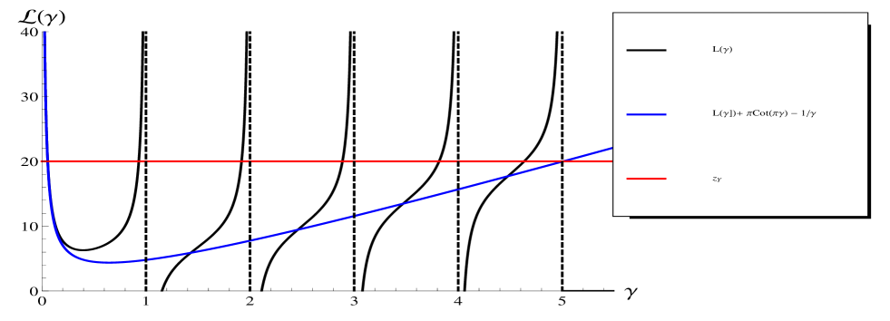
Figure 1: Function ${\cal L}\left(\gamma=d\phi\left(z\right)/dz\right)$ versus $\gamma$ (black line). Blue curve shows ${\cal L}\left(\gamma\right)+\pi\cot\left(\pi\gamma\right)-1/\gamma$ while the red one shows ${\cal L}\left(\gamma\right)=z_{Y}$.

1. For $z_{Y}\,>\,z_{Y}^{\mbox{min}}\,\approx 6.3$ there is a solution at $\phi^{\prime}_{z}\left(z\right)\,=\gamma\left(z\right)\,\ll\,1$ ( $\gamma\to 0$);

2. For all $z_{Y}$ we have solutions $\phi^{\prime}\left(z\right)\,\,=\,\,\,n\,z$ ($\gamma\to n$), where $n\,=\,1,2,3,\dots$;

3. For $z_{Y}\,>\,z_{Y}^{\mbox{min}}\,\approx 6.3$ we have the following solution:

   $$\phi\left(z\right)\,\,=\,\,\frac{1-\gamma_{cr}}{\chi\left(\gamma_{cr}\right)}\,z_{Y}\,z$$ (2.30)

In Fig. 1 the blue solid line shows

$$\tilde{\cal L}\,\,\equiv\,\,{\cal L}\left(\gamma\right)+\pi\cot\left(\pi\gamma\right)-1/\gamma.$$ (2.31)

All poles at $\gamma=n$ are excluded in this function while the behaviour at large $\gamma$ this function has the same as ${\cal L}\left(\gamma\right)$. This asymptotic behaviour at $\gamma$ close to $z_{Y}/C\left(\gamma_{cr}\right)$ can be translated in Eq. (2.30) (see also below Eq. (4.46) and Eq. (4.49)).

Therefore, one can see that we face two major problems in searching the solution: (i) at first sight we have infinite number of solutions even in this simplified case; and (ii) we need to find the solution if we exclude the singularities in ${\cal L}\left(\gamma\right)$.

The infinite number of solutions contradicts the common sense intuition that the physical problem has the only one solution being formulated correctly. In the next section 3 we show mathematical arguments that will discriminate different solutions and will select the only one solution. This physical solution will be found in section 4.

3 Semiclassical solution for $\phi\left(z,Y^{\prime}\right)$

3.1 Equations

For large $\phi\left(z,Y^{\prime}\right)$ Eq. (2.23) can be re-written in the form

$$\tilde{\omega}\,\,+\,\,{\cal L}\left(\gamma\right)\,\,-\,\,{\cal F}\left(\gamma\right)e^{-\phi}\,\,-\,\,z_{Y}\,\,=\,\,\tilde{\omega}\,\,+\,\,{\cal G}\left(\gamma,\phi\right)\,\,-\,\,z_{Y}\,\,=\,\,0$$ (3.32)

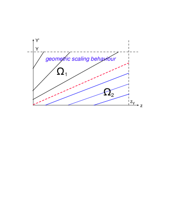
Figure 2: Two kinematic regions: $\Omega_{1}$ and $\Omega_{2}$. The solid lines describe two sets of trajectories in $\Omega_{1}$ and $\Omega_{2}$. The trajectories in $\Omega_{1}$ start at $z=0$ with given value of $\phi_{0}$. The trajectories in $\Omega_{2}$ start at any point of $z$ at $Y^{\prime}=0$. The initial value of $\gamma_{0}=\phi_{0}\,\exp\left(z_{0}\right)$. The dotted red line is the common characteristic line for both $\Omega_{1}$ and $\Omega_{2}$. It has the form (see Eq. (4.45) and Eq. (4.44) below): $Y^{\prime}=z/C\left(\gamma_{cr}\right)$ .

We solve this equation in semi-classical approximation assuming that $\phi\left(z,Y^{\prime}\right)$ is a smooth function of both variables $z$ and $Y^{\prime}$. It is known (see Refs. [22] and references therein) that for the equation in the form

$$F(Y^{\prime},z,\phi,\,\gamma,\tilde{\omega})=0$$ (3.33)

with smooth $\phi$. We can introduce the set of characteristic lines : $z(t),Y^{\prime}(t),\phi(t),$ $\tilde{\omega}(t),$ and $\gamma(t)$ which are the functions of the variable $t$ ( artificial time), that satisfy the following equations:

$$(1.)\,\,\,\,\frac{dz}{d\,t}\,\,=\,\,F_{\gamma}\,\,=\,\,\frac{\partial{\cal G}\left(\gamma,\phi\right)}{\partial\gamma}$$

$$(2.)\,\,\,\,\,\,\,\frac{d\,Y^{\prime}}{d\,t}\,\,=\,\,F_{\tilde{\omega}}\,\,=\,\,1\,\,\,\,\,\,\,$$ (3.34)

$$(3.)\,\,\,\,\frac{d\,\tilde{\phi}}{d\,t}\,\,=\,\,\gamma\,F_{\gamma}\,+\,\tilde{\omega}\,F_{\tilde{\omega}}\,\,=\,\,\,\,\gamma\frac{\partial{\cal G}}{\partial\gamma}\,\,+\,\,\tilde{\omega}$$

$$(4.)\,\,\,\,\frac{d\,\gamma}{d\,t}\,\,=\,\,-(\,F_{z}\,+\,\gamma\,F_{\phi}\,)\,\,=\,\,-\,\gamma\,{\cal F}\left(\gamma\right)\,e^{-\phi}$$

$$(5.)\,\,\,\,\frac{d\,\tilde{\omega}}{d\,t}\,\,=\,\,-\,(\,F_{Y^{\prime}}\,+\,\tilde{\omega}\,F_{\phi}\,)\,\,=\,\,-\,\tilde{\omega}\,{\cal F}\left(\gamma\right)\,e^{-\phi}$$

From Eq. (3.34)-2 one can see that we can introduce $t=Y^{\prime}$. Taking the ration of Eq. (3.34)-4 to Eq. (3.34)-5 we obtain that

$$\tilde{\omega}\left(Y^{\prime}\right)\,\,=\,\,{\cal K}\left(\gamma_{0}\right)\,\gamma\left(Y^{\prime}\right)$$ (3.35)

where $\gamma_{0}\,\equiv\,\gamma\left(Y^{\prime}=0\right)$ is the initial value of $\gamma$ which has to be found from the initial conditions.

Plugging Eq. (3.35) into Eq. (3.32) we reduce the system of equation (see Eq. (3.34)) to the following set of the equations:

$$e^{-\phi}\,\,=\,\,\Big{(}{\cal L}\left(\gamma\right)\,\,-\,\,z_{Y}\,\,+\,\,\gamma\,{\cal K}\left(\gamma_{0}\right)\Big{)}{\Big{/}}{\cal F}\left(\gamma\right);$$ (3.36)

$$dz\left(Y^{\prime}\right)/dY^{\prime}\,\,=\,\,{\cal L}_{\gamma}\left(\gamma\right)\,\,-\,\,{\cal F}_{\gamma}\left(\gamma\right)\,e^{-\phi};$$ (3.37)

$$d\gamma/dY^{\prime}\,=\,-\,\gamma\,\Big{(}{\cal L}\left(\gamma\right)+{\cal K}\left(\gamma_{0}\right)\,\gamma-z_{Y}\Big{)}\equiv T\left(\gamma,\gamma_{0}\right);$$ (3.38)

It turns out the general set of trajectories can be divided in two groups: the trajectories that start at $z=0$ and at arbitrary $Y^{\prime}$ ( the vertical axis in Fig. 2) and the trajectories which starting points lie on the horizontal axis in Fig. 2 at $Y^{\prime}$ and arbitrary $z$. We need to consider these two sets separately.

3.2 Solutions in $\Omega_{1}$

In $\Omega_{1}$ we need to use the initial condition $\phi\left(z=0\right)=\phi_{0}$ to obtain the equation for ${\cal K}\left(\gamma_{0}\right)$.

$${\cal K}\left(\gamma_{0}\right)\,\,=\,\,\frac{1}{\gamma_{0}}\Big{(}-\,{\cal L}\left(\gamma_{0}\right)\,\,+\,\,{\cal F}\left(\gamma_{0}\right)\,e^{-\phi_{0}}\,\,+\,\,z_{Y}\Big{)}$$ (3.39)

Substituting Eq. (3.39) into Eq. (3.36)-Eq. (3.38) we have the final set of equations for the trajectories in the region $\Omega_{1}$.

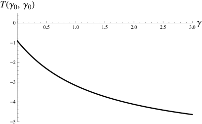
Figure 3: $T\left(\gamma_{0},\gamma_{0}\right)$ versus $\gamma_{0}$ in the region $\Omega_{1}$ . $N_{0}=0.1$ and $z_{Y}=200$.

In Fig. 3 we see that function ${\cal T}\left(\gamma_{0},\gamma_{0}\right)$ is negative for all values of $\gamma_{0}$. It means that $\gamma\left(Y^{\prime}\right)$ falls down and becomes frozen at the value $\bar{\gamma}_{0}\,=\,\gamma_{0,1}\left(\gamma_{0}\right)$ at which $T\left(\bar{\gamma}_{0},\gamma_{0}\right)\,=\,0$ (see Fig. 4). One can see that for $0\,<\,\gamma\,<\,1$ actually equation $T\left(\bar{\gamma}_{0},\gamma_{0}\right)\,=\,0$ has two solutions $\gamma_{0,1}$ and $\gamma_{0,2}$ but both are smaller than $\gamma_{0}$. For $\gamma\,>\,1$ we have the only one solution $\bar{\gamma}_{0}\,<\,\gamma_{0}$. Actually, $\bar{\gamma}_{0}$ is very close to $\gamma_{0}$. In other words, $\gamma$ decreases very fast to $\bar{\gamma}_{0}$. At $\gamma=\bar{\gamma}_{0}$ $T\left(\gamma=\bar{\gamma}_{0},\gamma_{0}\right)\,=\,0$. Since the scattering amplitude $N$ should be less that unity from the $s$-channel unitarity we expect that $\exp\left(-\phi\left(z,Y^{\prime}\right)\right)$ in entire kinematic region should be positive and not equal to zero.

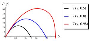
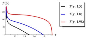
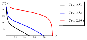
Fig. 4-a	Fig. 4-b	Fig. 4-c

Figure 4: $T\left(\gamma,\gamma_{0}\right)$ versus $\gamma$ for $\gamma_{0}=0\dots 1$(Fig. 4-a), for $\gamma=1\dots 2$( Fig. 4-b) and $\gamma=2\dots 3$(Fig. 4-c) in the region $\Omega_{1}$. $N_{0}=0.1$ and $z_{Y}=200$.

Fig. 5 shows that we have a different behaviour of the solution for $\exp\left(-\phi\big{(}z\left(Y^{\prime}\right)\right)\big{)}$ on the trajectories, which contradicts our expectation from the physics point of view.

Therefore, we can conclude that the semi-classical solution that satisfies the physical criterion, does not exist at any $\gamma_{0}$ in the region $\Omega_{1}$ when $\gamma$ close to $n$ with $n=0,1,2,3,\dots$.

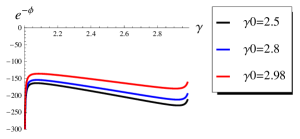
Fig. 5-a	Fig. 5-b	Fig. 5-c

Figure 5: $\exp\left(-\phi\left(\gamma,\gamma_{0}\right)\right)$ versus $\gamma$ for $\gamma_{0}=0\dots 1$(Fig. 5-a), for $\gamma=1\dots 2$( Fig. 5-b) and $\gamma=2\dots 3$(Fig. 5-c) in the region $\Omega_{1}$. $N_{0}=0.1$ and $z_{Y}=200$.

3.3 Solutions in $\Omega_{2}$

In the region $\Omega_{2}$ we have to repeat our analysis since the equation for ${\cal K}\left(\gamma_{0}\right)$ should be based on the initial condition: $\phi\left(z=z_{0},Y^{\prime}=0\right)\,=\,\phi_{0}\exp\left(z_{0}\right)$. Since $\gamma_{0}=\phi\left(z=z_{0},Y^{\prime}=0\right)$ for this initial condition Eq. (3.39) can be re-written in the form

$${\cal K}\left(\gamma_{0}\right)\,\,=\,\,\frac{1}{\gamma_{0}}\Big{(}-\,{\cal L}\left(\gamma_{0}\right)\,\,+\,\,{\cal F}\left(\gamma_{0}\right)\,e^{-\gamma_{0}}\,\,+\,\,z_{Y}\Big{)}$$ (3.40)

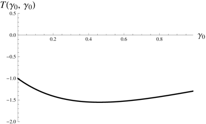
Figure 6: $T\left(\gamma_{0},\gamma_{0}\right)$ versus $\gamma_{0}$ in the region $\Omega_{2}$. $N_{0}=0.1$ and $z_{Y}=200$.

One can see in Fig. 6 that $T\left(\gamma_{0},\gamma_{0}\right)$ in this region is negative. Therefore, in this region as in region $\Omega_{1}$ $\gamma\left(z\right)$ falls down on the trajectory for all trajectories. It turns out that for each value of $\gamma_{0}$ function $T\left(\gamma,\gamma_{0}\right)$ vanishes at $\bar{\gamma}_{0}=\gamma_{0,1}\left(\gamma_{0}\right)$ ($T\left(\bar{\gamma}_{0},\gamma_{0}\right)=0$) (see Fig. 7). Therefore, the solution in region $\Omega_{2}$ has the same properties as the solution in region $\Omega_{1}$ (see Fig. 7 and Fig. 8.

Thus we can repeat the same conclusions for the region $\Omega_{2}$ as for $\Omega_{1}$: there is no solutions that satisfy the physical criteria.

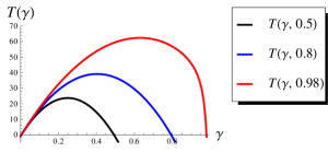
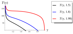
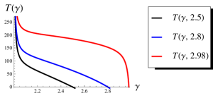
Fig. 7-a	Fig. 7-b	Fig. 4-c

Figure 7: $T\left(\gamma,\gamma_{0}\right)$ versus $\gamma$ for $\gamma_{0}=0\dots 1$(Fig. 7-a), for $\gamma=1\dots 2$( Fig. 7-b) and $\gamma=2\dots 3$(Fig. 7-c) in the region $\Omega_{2}$. $N_{0}=0.1$ and $z_{Y}=200$.

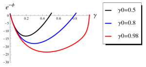
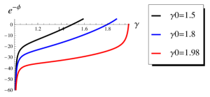
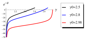
Fig. 8-a	Fig. 8-b	Fig. 8-c

Figure 8: $\exp\left(-\phi\left(\gamma,\gamma_{0}\right)\right)$ versus $\gamma$ for $\gamma_{0}=0\dots 1$(Fig. 8-a), for $\gamma=1\dots 2$( Fig. 8-b) and $\gamma=2\dots 3$(Fig. 8-c) in the region $\Omega_{2}$. $N_{0}=0.1$ and $z_{Y}=200$.

4 Asymptotic solution with $\gamma\longrightarrow z_{Y}\Big{/}\left(\bar{\alpha}_{S}\,\frac{\chi\left(\gamma_{cr}\right)}{1-\gamma_{cr}}\right)$

Finally, the only solution which we need to consider is the solution with large $\gamma=d\phi\left(z,Y^{\prime}\right)/dz\to z_{Y}/C\left(\gamma_{cr}\right)\gg 1$. Eq. (2.23) reduces to the simple form

$$\frac{\partial\phi\left(z,Y^{\prime}\right)}{\partial\bar{\alpha}_{S}Y^{\prime}}\,\,+\,\,C\left(\gamma_{cr}\right)\frac{\partial\phi\left(z,Y^{\prime}\right)}{\partial z}\,\,=\,\,z_{Y}~{}~{}~{}~{}~{}~{}~{}~{}~{}~{}~{}~{}\mbox{where}~{}~{}~{}~{}~{}~{}~{}~{}~{}C\left(\gamma_{cr}\right)\,\,=\,\,\frac{\chi\left(\gamma_{cr}\right)}{1\,-\,\gamma_{cr}}$$ (4.41)

with the following initial conditions:

$$\phi\left(z\,=\,0,Y^{\prime}\right)\,\,=\,\,\phi_{0}\,;~{}~{}~{}~{}~{}~{}~{}~{}~{}~{}~{}~{}~{}~{}~{}~{}~{}~{}~{}\phi\left(z,Y\,=\,0^{\prime}\right)\,\,=\,\,\phi_{0}\,e^{z};$$ (4.42)

We need to consider two separate kinematic regions $\Omega_{1}$ and $\Omega_{2}$ for searching the solutions for this equation (see Fig. 2): $Y^{\prime}\,\geq\,z/C\left(\gamma_{cr}\right)$ and $Y^{\prime}\,\leq\,z/C\left(\gamma_{cr}\right)$ [23]. In both regions the general solution to Eq. (4.41) takes the form

$$\phi\left(z,Y^{\prime}\right)\,\,=\,\,\frac{1}{2}\,z_{Y}\,\left(Y^{\prime}\,+\,z/C\left(\gamma_{cr}\right)\right)\,\,+\,\,G\left(Y^{\prime}\,-\,z/C\left(\gamma_{cr}\right)\right)$$ (4.43)

where $G$ is the arbitrary function that has to be found from Eq. (4.42). In region $\Omega_{2}$ one can see that

$$G_{2}\,=\,\phi_{0}\,\exp\Big{(}-C\left(\gamma_{cr}\right)\,\left(Y^{\prime}\,-\,z/C\left(\gamma_{cr}\right)\right)\Big{)}$$ (4.44)

from the second of Eq. (4.42). However, in region $\Omega_{1}$ we need to use the first of Eq. (4.42) and we obtain that

$$G_{1}\,\,=\,\,-\frac{1}{2}\,z_{Y}\,\left(Y^{\prime}\,-\,z/C\left(\gamma_{cr}\right)\right)\,\,+\,\,\phi_{0}$$ (4.45)

One can see that at $Y^{\prime}=z/C\left(\gamma_{cr}\right)$ two $\phi$’s: $\phi_{1}\left(z\right)\,\,=\,\,z_{Y}\,z\,\,+\,\,\phi_{0}$ and $\phi_{2}\left(z,Y^{\prime}\right)\,\,=\,\,\frac{1}{2}\,z_{Y}\,\left(Y^{\prime}\,+\,z/C\left(\gamma_{cr}\right)\right)\,\,+\phi_{0}\,\exp\Big{(}-C\left(\gamma_{cr}\right)\,\left(Y^{\prime}\,-\,z/C\left(\gamma_{cr}\right)\right)\Big{)}$ are equal, providing the needed matching.

Therefore, the simplified Eq. (4.41) leads to the geometric scaling solution for $Y^{\prime}\,\,\geq\,\,z/C\left(\gamma_{cr}\right)$ while for $Y^{\prime}\,\,\leq\,\,z/C\left(\gamma_{cr}\right)$ we have a solution with explicit scaling violation.

Armed with the asymptotic solution given by Eq. (4.45) and Eq. (4.44) we study the numerical solution to Eq. (2.23) in region $\Omega_{1}$ assuming the geometric scaling behaviour and considering the following iterative procedure. Plugging in Eq. (2.23) $\phi\left(z,Y^{\prime}\right)=\phi\left(z\right)$ and Eq. (2.31) we see that this equation takes the following form in this region

$$\frac{\chi\left(\gamma_{cr}\right)}{1-\gamma_{cr}}\,\frac{d\phi^{(i)}\left(z\right)}{dz}\,\,-\,\,2\left(\gamma_{E}+\ln\left(\frac{d\phi^{(i)}\left(z\right)}{dz}\right)\right)\,\,=\,\,z_{Y}\,\,\,-\,\,H\left(z\right)\,-\,H\left(z_{Y}-z\right)\,\,\,\,\,\mbox{with}\,\,\,\,\,H\left(z\right)\,\,=\,\,\int^{z}_{0}dz^{\prime}e^{-\phi^{(i-1)}\left(z^{\prime}\right)}$$ (4.46)

where $\gamma_{E}$ is the Euler constant ($\gamma_{E}\,=\,0.5777216$) and where $\phi^{(i)}$ is the solution of the $i$-th iteration of the equation. Deriving Eq. (4.46) we used that $\tilde{\cal L}\,\xrightarrow{\gamma\gg 1}\,\gamma_{E}\,+\,\ln\left(\gamma\right)$.

We solve Eq. (4.46) using iteration procedure with

$$\phi^{(i=0)}\,=\,\Big{\{}\left(z_{Y}\,+\,2\left(\gamma_{E}+\ln z_{Y}\right)\right)(1-\gamma_{cr})/\chi\left(\gamma_{cr}\right)\Big{\}}\,z.$$ (4.47)

The result of the third iteration is shown in Fig. 9. One can see from Fig. 9-a that the solution is very close to $\phi^{(0)}$ given by Eq. (4.47). $N^{\prime}_{z}$ reaches the unitarity limit at small values of $z$($z\leq 0.5$). In Fig. 9-c we plotted the difference between the l.h.s. and the r.h.s. of Eq. (2.23). This difference can be written in the form:

$$T^{(i)}\left(z\right)\,\,=$$ (4.48)

$$\,\,{\cal L}\left(\phi^{\prime(i)}_{z}\left(z\right)\right)-{\cal F}\left(\phi^{\prime(i)}_{z}\left(z\right)\right)\,e^{-\phi^{(i)}\left(z\right)}\,\,-\,\,\tilde{N}^{(i)}\left(z\right)\,\,-\,\,\tilde{N}^{(i)}\left(z_{Y}-z\right)$$

$$\mbox{where}\,\,\,\,e^{-\phi^{(i)}}\,\,=\,\,1-d\tilde{N}^{(i)}\left(z\right)/dz\,\,\,\,\mbox{and}\,\,\,\,d\phi^{(i)}/dz\,\,=\,\,\frac{d^{2}\tilde{N}^{(i)}\left(z\right)}{dz^{2}}/\left(1-d\tilde{N}^{(i)}\left(z\right)/dz\right)$$

$T^{(i)}\left(z\right)$ turns out to be small ( less than 1) leading to the accuracy of the solution about 2%.

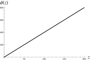
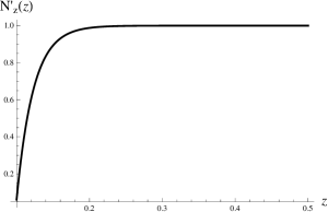
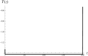
Fig. 9-a	Fig. 9-b	Fig. 9-c

Figure 9: The third iteration of Eq. (4.46): solutions for functions $\phi\left(z\right)$(Fig. 9-a) and the scattering amplitude $N^{\prime}_{z}\left(z\right)$ (Fig. 9-b) versus $z$.   In Fig. 9-c we plot function $T\left(z\right)$ (see Eq. (4.48)). In the figure the following parameters are taken: $N_{0}=0.1$ and $z_{Y}=200$.

For the region $\Omega_{2}$ (see Fig. 2) we solve a more general equation for $\phi\left(z,Y^{\prime}\right)$. In this case Eq. (4.46) takes the form

$$\frac{\partial\phi\left(z,Y^{\prime}\right)}{\partial\bar{\alpha}_{S}Y^{\prime}}\,\,+\,\frac{\chi\left(\gamma_{cr}\right)}{1-\gamma_{cr}}\,\frac{\partial\phi\left(z,Y^{\prime}\right)}{\partial z}\,\,-\,\,2\left(\gamma_{E}+\ln\left(\frac{d\phi\left(z,Y^{\prime}\right)}{dz}\right)\right)\,\,=\,\,z_{Y}\,\,+4\,N_{0}\,\,-\,\,H\left(z,Y^{\prime}\right)\,-\,H\left(z_{Y}-z,Y-Y^{\prime}\right)$$ (4.49)

where $\,H\left(z,Y^{\prime}\right)\,\,=\,\,\int^{z}_{0}dz^{\prime}e^{-\phi\left(z^{\prime},Y^{\prime}\right)}$. The initial conditions are given by Eq. (4.42).

The numerical solution is shown in Fig. 10. One can see that at large values of $Y^{\prime}$ solution approaches the geometric scaling solution of Eq. (4.46). We can use this physical solution, shown in Fig. 10 and Fig. 9, to study the N-N scattering in the next section.

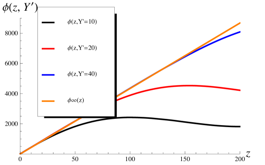
Figure 10: Function $\phi\left(z,Y^{\prime}\right)$ at different values of $Y^{\prime}$ as function of $z$. In the figure the following parameters are taken: $N_{0}=0.1$ and $z_{Y}=200$

5 Nucleus-nucleus scattering amplitude

We need to specify term $S_{E}$ in Eq. (2.1) for calculating the scattering amplitude with a nucleus. This term determines the interaction of the BFKL Pomeron with the nucleons of the nucleus and it has been written in Ref.[1] in the following form

$$S_{E}\,\,=\,\,\int d^{2}b\,d^{2}k\,\Big{(}\Phi\left(k,b,Y^{\prime}=0\right)\tau_{A_{2}}\left(k,b\right)\,\,\,+\,\,\,\Phi^{\dagger}\left(k,b,Y^{\prime}=Y\right)\tau_{A_{1}}\left(k,b\right)\Big{)}$$ (5.50)

where

$$\tau_{A}\left(k,b\right)\,\,=\,\,S_{A}\left(b\right)\,\sigma\left(k\right)\,\,\,\,\mbox{with}\,\,\,\,\,S_{A}\left(b\right)\,\,=\,\,\int^{+\infty}_{-\infty}\,d\,z\,\rho\left(z,b\right)\,\,\,\,\mbox{and}\,\,\,\,\sigma\left(k\right)\,=\,\int n\left(k,b\right)d^{2}b$$ (5.51)

In Eq. (5.51) $\rho$ is the density of the nucleons in the nucleus and $\sigma\left(k\right)$ is the cross section (imaginary part of the forward scattering amplitude) of the dipole with the nucleon at low energy while $n\left(k,b\right)$ is the dipole-nucleon scattering amplitude.

As we have eluded, in our treatment of nucleus-nucleus interaction we use the Glauber-type approach[26] integrating over all impact parameters of dipole-dipole and dipole-nucleon interaction since they are assumed to be much smaller than the impact parameters of nucleon-nucleon scattering (see for example Ref.[27] in which this approach is discussed in details). The latter is of the order of $R_{A}$, which is larger than the nucleon radius and the sizes of all interacting dipoles. As we have discussed, we assume that instead of the real nuclei we are dealing with the nuclei that consist of mesons made of heavy quark and antiquarks. For such mesons we can calculate $n\left(k\right)$ in the Born Approximation of perturbative QCD. In coordinate space $n\left(r\right)=\left(2\pi\alpha_{S}^{2}C_{F}/N_{c}\right)r^{2}\ln\left(R^{2}/r^{2}\right)\,\Theta\left(R-r\right)$ where $R$ is the radius of the meson which is of the order of $1/\left(\alpha_{S}\left(M_{Q}\right)M_{Q}\right)$ where $M_{Q}$ is the mass of heavy quark. In the momentum space we have the following $\tau_{A}\left(k,b\right)$

$$\tau_{A}\left(k,b\right)\,\,\,=\,\,\,S_{A}\left(b\right)\,\sigma\left(k\right)\,\,=\,\,S_{A}\left(b\right)\,\frac{\alpha_{S}^{2}C_{F}}{\pi N_{c}}\,\frac{1}{k^{2}\,+\,\alpha_{S}^{2}\,M^{2}_{Q}}$$ (5.52)

$\tau$ determine the initial conditions for the amplitude $N\left(k,b,Y^{\prime}\right)$ and $N^{\dagger}\left(k,b,Y^{\prime}\right)$, namely

$$N\left(k,b,Y^{\prime}=0\right)\,\,=\,\,\tau_{A_{1}}\left(b,k\right)\,;\,\,\,\,\,\,\,\,N^{\dagger}\left(k,b,Y^{\prime}=Y\right)\,\,=\,\,\tau_{A_{2}}\left(b,k\right)\,;$$ (5.53)

For simplicity, we consider the cylindric nuclei for which the $b$ dependence is given by $\Theta\left(R_{A}-b\right)$. In this model

$$S_{A}\left(b\right)\,\,=\,\,2\,\rho_{0}\,R_{A}\,\Theta\left(R_{A}-b\right)$$ (5.54)

In this simple model the entire $b$ dependence of $N\left(k,b,Y^{\prime}\right)$ and $N^{\dagger}\left(k,b,Y^{\prime}\right)$ turns out to be the same as in initial condition leading to

$$N\left(k,b,Y^{\prime}\right)\,\, = \,\,S_{A}\left(b\right)\,{\cal\sigma}\left(k,Y^{\prime}\right)\,\,=\,\,S_{A}\left(b\right)\,\frac{1}{k^{2}_{0}}{\cal N}\left(k,Y^{\prime}\right)$$

$$N^{\dagger}\left(k,b.Y^{\prime}\right)\,\, = \,\,S_{A}\left(b\right)\,{\sigma}^{\dagger}\left(k,Y^{\prime}\right)\,\,=\,\,S_{A}\left(b\right)\,\frac{1}{k^{2}_{0}}{\cal N}^{\dagger}\left(k,Y^{\prime}\right)$$ (5.55)

where $k_{0}$ is the typical transverse momentum in the proton ($k_{0}\propto\,\alpha_{S}M_{Q}$). Functions ${\cal N}$ and ${\cal N}^{\dagger}$ are dimensionless and for them we have the geometric scaling behaviour inside the saturation region [20] and in the vicinity of the saturation outside of the saturation region[19].

Using $\rho\left(z=0,b=0\right)=\rho_{0}=0.171/fm^{3}$ and $R_{A}=1.2\,A^{1/3}\,fm$ we can estimate the value of $\tau$ at $k=0$ for the gold: $\tau=8\rho_{0}\,R_{A}/(9\pi\,M^{2}_{Q})\,\,=\,\,0.32(1/fm^{2})/M^{2}_{Q}$ . One can see that $N_{0}=0.1$ which we used for the numerical solution can be reached even at $k=0$ if $M_{Q}\approx 0.36\,GeV$.

Calculating the scattering amplitude, we need first to sum all two nuclei reducible diagrams (see Fig. 11 for example). In such diagrams we can single out one or more states with two nuclei in the $s$-channel (see, for example, two such states in Fig. 11).

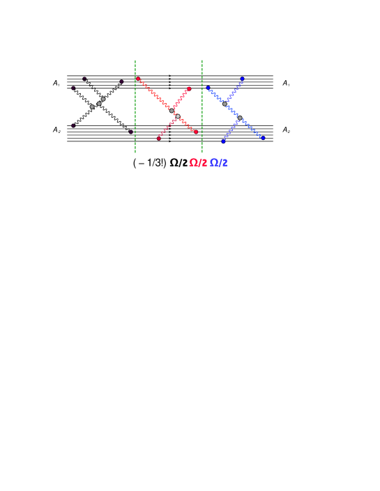
Figure 11: The example of two nuclei reducible diagram in the scattering amplitude for nucleus-nucleus interaction.

This sum can be written as follows

$$ImA\left(b,Y\right)\,\,=\,\,\Big{(}1\,\,\,-\,\,e^{-\frac{1}{2}\Omega\left(b,Y\right)}\Big{)}$$ (5.56)

The notation : $\Omega$ in Eq. (5.56), is introduced to be opacity for the nucleus-nucleus scattering in the Glauber-Gribov approach[26].

Using Eq. (5.50) one can see that the equation for the opacity $\Omega$ has the following form (see Fig. 12)

$$\Omega\left(b,Y\right)\,=\,\int d^{2}b^{\prime}\,d^{2}k\,\tau_{A_{1}}\left(\vec{b}\,-\,\vec{b}^{\prime},k\right)\,N\left(b^{\prime},k,Y^{\prime}=Y\right)\,=\,\int d^{2}b^{\prime}\,d^{2}k\,N^{\dagger}\left(\vec{b}\,-\,\vec{b}^{\prime},k,Y^{\prime}=0\right)\,\tau_{A_{2}}\left(b^{\prime},k\right)$$ (5.57)

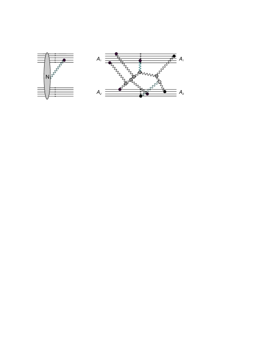
Figure 12: The equation for opacity $\Omega$.

Plugging in Eq. (5) we can rewrite Eq. (5.57) in the form

$$\Omega\left(b,Y\right)\,=\,T_{AA}\left(b\right)\int\,d^{2}k\,\sigma\left(\vec{b}\,-\,\vec{b}^{\prime},k\right)\,{\sigma}\left(k,Y^{\prime}=Y\right)\,\,=\,\,T_{AA}\left(b\right)\,\frac{1}{k^{2}_{0}}\int\,d^{2}k\,\sigma\left(\vec{b}\,-\,\vec{b}^{\prime},k\right)\,{\cal N}\left(k,Y^{\prime}=Y\right)$$ (5.58)

where

$$T_{AA}\left(b\right)\,\, = \left(2\rho_{0}R_{A}\right)^{2}\,\,\int d^{2}b^{\prime}\Theta\left(b^{\prime}-R_{A}\right)\Theta\left(|\vec{b}-\vec{b}^{\prime}|-R_{A}\right)\,\,$$

$$= \,\,\left(2\rho_{0}R_{A}\right)^{2}\,R^{2}_{A}\left(2\,\arccos\left(\frac{b}{2\,R_{A}}\right)-\frac{b}{2\,R_{A}}\sqrt{1-\frac{b^{2}}{4\,R^{2}_{A}}}\,\,\right)$$

As we have discussed the solution for ${\cal N}\left(z\right)$ at $z\leq z_{min}$ and ${\cal N}^{\dagger}\left(Z_{y}-z\right)$ for $z_{Y}-z\leq z_{min}$ are the solution to the linear BFKL equation which can be written in the following form

$$0\,\leq\,z\,\leq z_{min}\,\,\,\,\,\,\,\,\, N\left(k,Y\right)=\frac{1}{k^{2}_{0}}{\cal N}\left(z\right) =\,\,\int\,d^{2}k^{\prime}\,\sigma\left(k^{\prime}\right)\,{\sigma}_{BFKL}\left(k/k^{\prime},Y^{\prime}=Y\right)$$

$$=\,\,\frac{\alpha_{S}^{2}C_{F}}{\pi\,N_{c}}\frac{1}{k^{2}_{0}}\int\frac{dk^{\prime 2}}{k^{\prime 2}\,+\,\alpha_{S}^{2}M^{2}_{Q}}\,{\cal N}_{BFKL}\left(k/k^{\prime},Y^{\prime}=Y\right)$$

$$0\,\leq\,z_{Y}-z\,\leq\,z_{min}\,\,\,\,\,\,\,\,\, N^{\dagger}\left(k,Y\right)\,=\,\frac{1}{k^{2}_{0}}{\cal N}^{\dagger}\left(z\right) =\,\,\int\,d^{2}k^{\prime}\,\sigma\left(k^{\prime}\right)\,{\cal\sigma}^{\dagger}_{BFKL}\left(k/k^{\prime},Y^{\prime}=Y\right)$$

$$=\frac{\alpha_{S}^{2}C_{F}}{\pi\,N_{c}}\frac{1}{k^{2}_{0}}\int\frac{dk^{\prime 2}}{k^{\prime 2}\,+\,\alpha_{S}^{2}M^{2}_{Q}}\,{\cal N}^{\dagger}_{BFKL}\left(k/k^{\prime},Y^{\prime}=Y\right)$$

In the vicinity of the saturation scale ${\cal N}_{BFKL}$ and ${\cal N}^{\dagger}_{BFKL}$ in Eq. (5) and Eq. (5) can be written in the simple form [20]:

$${\cal N}_{BFKL}\left(k/k^{\prime},Y^{\prime}=Y\right)\,\,=\,\,N_{0}\,e^{\left(1-\gamma_{cr}\right)z^{\prime}}\,\,\,\,\,\mbox{and}\,\,\,\,\ {\cal N}^{\dagger}_{BFKL}\left(k/k^{\prime},Y^{\prime}=Y\right)\,\,=\,\,N_{0}\,e^{\left(1-\gamma_{cr}\right)\left(z_{Y}-z^{\prime}\right)}$$ (5.62)

where

$$z^{\prime}\,\,=\,\,\bar{\alpha}_{S}\,\frac{\chi\left(\gamma_{cr}\right)}{1-\gamma_{cr}}\,Y\,\,-\,\,\ln\left(k^{2}/k^{\prime 2}\right)\,$$ (5.63)

Taking the integration over $k^{\prime}$ in Eq. (5) and Eq. (5) we obtain:

$$0\,\leq\,z\,\leq z_{min}\,\,\,\,\,\,\,\,\, {\cal N}\left(z\right) =\,\,\frac{\alpha_{S}^{2}C_{F}}{\pi\,N_{c}}\frac{N_{0}}{1-\gamma_{cr}}\exp\Big{(}\left(1-\gamma_{cr}\right)z\Big{)}$$

$$0\,\leq\,z_{Y}-z\,\leq\,z_{min}\,\,\,\,\,\,\,\,\, {\cal N}^{\dagger}\left(z\right) =\,\,\,\frac{\alpha_{S}^{2}C_{F}}{\pi\,N_{c}}\frac{N_{0}}{1-\gamma_{cr}}\exp\Big{(}\left(1-\gamma_{cr}\right)\left(z_{Y}-z\right)\Big{)}$$ (5.64)

It should be noticed that in the above equations $l$ is defined as $l=\ln\left(k^{2}/(\alpha_{S}M_{Q})^{2}\right)$ (see Eq. (2.18) and Eq. (2.11)) with $k^{2}_{0}=(\alpha_{S}M_{Q})^{2}$.

Having these equation in mind we use a generalization of Eq. (5.58)

$$\Omega\left(b;Y\right)\,\,=\,\,T_{AA}\left(b\right)\int dl\,\,{\cal N}^{\dagger}\left(Y-Y^{\prime};L-l\right)\,{\cal N}\left(Y^{\prime};l\right)$$ (5.65)

Eq. (5.65) has been proposed and discussed in Ref.[17] and for the nucleus-nucleus scattering it is illustrated by Fig. 13. From this figure one can see that arbitrary BFKL Pomeron diagram for the case of nucleus-nucleus scattering can be written as the product of $N^{\dagger}N$. The extra Pomeron contribution that could connect two sets of diagrams for $N^{\dagger}$ and $N$(shown in black for $N$ and in red for $N^{\dagger}$ in Fig. 13) leads to a small corrections (see Ref.[4] for details). $Y^{\prime}$ is the arbitrary rapidity which is chosen from the condition $z=z_{min}$.

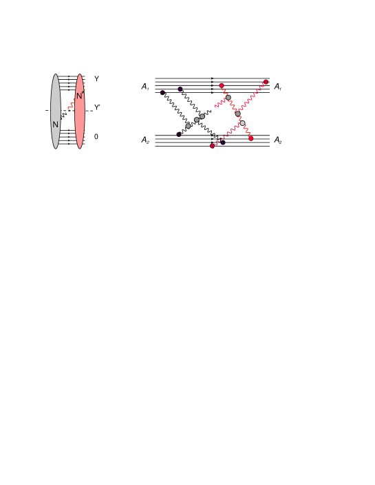
Figure 13: Graphic form of Eq. (5.65). Solid black lines denote the Pomerons and their interactions that contribute to $N$, while the same contributions for $N^{\dagger}$ are shown in red.

Using Eq. (4.44) for ${\cal N}^{\dagger}\left(Y-Y^{\prime};L-l\right)$ we can reduce Eq. (5.65) to the form

$$\Omega\left(b,z_{Y}\right)\,=\,T_{AA}\left(b\right)\,\frac{\alpha_{S}^{2}C_{F}}{\pi\,N_{c}\,\left(\alpha_{S}M_{Q}\right)^{2}}\frac{N_{0}}{1-\gamma_{cr}}\,\int_{z_{Y}+z_{min}}dz\,e^{\left(1-\gamma_{cr}\right)\left(z_{Y}-z\right)}\,{\cal N}\left(z\right)$$ (5.66)

This equation stems from the geometric scaling behaviour of the solution to the equations for $N$ and $N^{\dagger}$.

In the kinematic region $z\leq 2z_{min}$ both ${\cal N}$ and ${\cal N}^{\dagger}$ in Eq. (5.65) are the solution of the BFKL equation and $\Omega$ in this region can be written as follows using Eq. (2.12):

$$z_{Y}\,\,\leq\,2\,z_{min}:\,\,\,\,\,\,\Omega\left(b,z_{Y}\right)\,=\,\frac{T_{AA}\left(b\right)}{\left(\alpha_{S}M_{Q}\right)^{2}}\,\Big{(}\frac{\alpha_{S}^{2}C_{F}}{\pi\,N_{c}}\Big{)}^{2}\frac{N^{2}_{0}}{\left(1-\gamma_{cr}\right)^{2}}\exp\left(\left(1-\gamma_{cr}\right)z_{Y}\right)$$ (5.67)

For large $z\,>\,2\,z_{min}$ $N(z)$ is given by solution of Eq. (4.46). For estimates we can use for $N\left(z\right)$ in this region the solution in the form

$${\cal N}_{z>z_{min}}\left(z\right)\,\,=\,\,\int^{z}_{z_{min}}d\,z^{\prime}\Big{(}1\,\,-\,\,e^{-\phi^{(i=0)}\left(z^{\prime}\right)}\Big{)}\,\,+\,\,{\cal N}\left(z_{min}\right)$$ (5.68)

where $\phi^{(i=0)}$ is given by Eq. (4.47). The expression for $\Omega$ reads as follows

$$z_{Y}\,\,\geq\,\,2\,z_{min}: \Omega\left(b,z_{Y}\right)\,=\,\frac{T_{AA}}{\,\left(\alpha_{S}M_{Q}\right)^{2}}\Big{(}\frac{\alpha_{S}^{2}C_{F}}{\pi\,N_{c}}\Big{)}^{2}\,\frac{N_{0}}{1-\gamma_{cr}}\Big{\{}\int^{z_{Y}-z_{min}}_{z_{min}}d\,z\int^{z}_{z_{min}}d\,z^{\prime}\Big{(}1\,\,-\,\,e^{-\phi^{(i=0)}\left(z^{\prime}\right)}\Big{)}$$ (5.69)

$$+\frac{N_{0}}{(1-\gamma_{cr})}\exp\Big{(}2\,(1-\gamma_{cr})\,z_{min}\Big{)}\Big{\}}$$

The result of our estimates using Eq. (5.67) - Eq. (5.69) is plotted in Fig. 14. One can see that starting with small values of $z_{Y}\geq 8$ the amplitude at $b=0$ is close to the unitarity bound (see red line in Fig. 11). For comparison we plot in Fig. 14 also the amplitude which corresponds to the the exchange by one BFKL Pomeron in nucleon-nucleon scattering:

$$A_{P}\left(AA;z_{Y},b\right)\,\,=\,\,i\,\Big{(}1\,\,-\,\,\exp\left(-\frac{1}{2}\Omega_{P}\left(z_{Y},b\right)\right)\Big{)}$$ (5.70)

with $\Omega_{P}\left(z_{y},b\right)$ given by Eq. (5) at any value of $z_{Y}$.

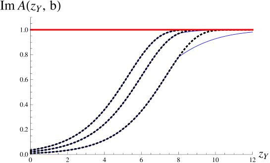
Figure 14: The scattering amplitude for gold-gold interaction versus $z\equiv z_{Y}$ at different values of $b$: the solid black line line is the result of this paper (see Eq. (5.69)), the red dotted curve describes the Glauber-Gribov formula for one BFKL Pomeron exchange (see Eq. (5.70)); and the red line shows the unitarity bound. The curves correspond $b=0,5\,fm$ and $10\,fm$ going from left to right,

The main conclusions that we can make from Fig. 14 is the fact that the exact solution for nucleus-nucleus scattering shows the same corrections as Glauber-Gribov formula. This happens because at $z_{Y}=2z_{min}$ the amplitude turns out to be very close to the unitarity bound. However, it should be stress that actually the exact solution leads to slower approaching to the unitarity bound since it turns out (see Fig. 15) that $\Omega\left(z_{Y},b\right)$ of Eq. (5.66) is much smaller than $\Omega_{P}\left(z_{Y},b\right)$ of Eq. (5.67) that corresponds to the exchange of one BFKL Pomeron at the entire kinematic region.

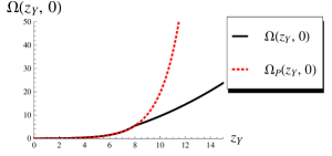
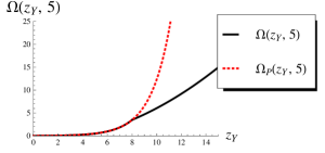
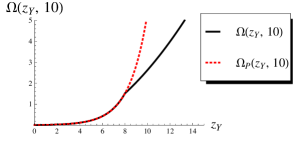
Figure 15: The opacity $\Omega\left(z_{Y},b\right)$ of Eq. (5.69) and $\Omega_{P}\left(z_{Y}\right)$ of Eq. (5) for gold-gold interaction at different $b$ versus $z\equiv z_{Y}$: black line is the result of this paper (see Eq. (5.67)), the red dotted curve describes the contribution to $\Omega$ from exchange of one BFKL Pomeron. The values of $b$ are given in $fermi$.

6 Conclusions

The main result of this paper is the solution in the form of Eq. (2.21) for amplitude $N\left(Y,Y^{\prime},l\right)=N\left(z,Y^{\prime}\right)$ with $\phi\left(z,Y^{\prime}\right)$ given by Eq. (4.43) and Eq. (4.46) and with the initial function $\phi^{(0)}\left(z,Y^{\prime}\right)$ determined by Eq. (4.42). We obtained this solution in two steps. First, we assume that Eq. (2.14) ($N\left(l,b;Y;Y_{0}\right)\,=\,N^{\dagger}\left(b;L-l,Y-Y_{0}\right)$) which is correct for the linear equation, is valid for the solution of the non-linear one. This conjecture allows us to reduce the system of two equations to one functional differential equation. Second, we solve this equation. The semi-classical approach was used to select out the infinite number of parasite solutions and the final solution was found analytically at large values of $Y^{\prime}$ as well as numerically in the entire region of Y’.

The solution, that has been found, looks as being different from the numerical solutions found in Refs.[2, 3], but it shares with them several common features. In particular, this solution exists only and $z\leq z_{min}\approx 4$. In our solution the amplitude $N^{\dagger}\left(Y,Y^{\prime},l\right)\,=\,N\left(z_{Y}-z\right)$. We have no proof that this solution is unique but we believe that the physics problem has the only one solution.

Using this solution we found the nucleus-nucleus scattering amplitude as a function of energy for ‘theoretical’ nuclei. This ’theoretical’ nucleus consists of the dipoles that are made of heavy quarks and antiquarks. We can use the perturbative QCD treating this nucleus. In reconstruction of the scattering amplitude we use Eq. (5.65) (see Fig. 12) which is the form of $t$-channel unitarity constraints and follows from Eq. (5.50) for $S_{E}$ term in the action of Eq. (2.1).

We showed that for $z_{Y}\,\leq\,2z_{min}$ the exact calculation give the same result as the Glauber-Gribov formula which is widely used for nucleus-nucleus scattering. It turns out that $z_{min}\approx 4$ is so large that our estimates lead to the result close to the Glauber-Gribov formula in the entire kinematic region of energies. Only at large impact parameters the exact formula for nucleus-nucleus scattering gives visible deviations from the estimates based on Glauber-Gribov approach. We believe that this observation is important for all practical estimates based on Glauber-Gribov approach.

In spite of the fact that the solved problem is still far away from the real physics environment we hope that our solution gives a reasonable first approximation to approach the nucleus-nucleus scattering for the nuclei that exist in reality.

7 Acknowledgements

We thank all participants of the HEP seminar at UTFSM for useful discussions. This research was supported by the Fondecyt (Chile) grants 1100648, 1095196 and DGIP 11.11.05.

References

- [1] M. A. Braun, Phys.Lett. B 483 (2000) 115, [arXiv:hep-ph/0003004]; Eur.Phys.J C 33 (2004) 113 [arXiv:hep-ph/0309293] ; Phys. Lett. B 632 (2006) 297, [Eur. Phys. J. C 48 (2006) 511], [arXiv:hep-ph/0512057].
- [2] S. Bondarenko and L. Motyka, Phys. Rev. D 75 (2007) 114015 [arXiv:hep-ph/0605185].
- [3] S. Bondarenko and M. A. Braun, Nucl. Phys. A 799 (2008) 151 [arXiv:0708.3629 [hep-ph]].
- [4] A. Kormilitzin, E. Levin, J. S. Miller, Nucl. Phys. A859 (2011) 87-113. [arXiv:1009.1329 [hep-ph]].
- [5] C. Contreras, E. Levin and J. S. Miller, Nucl. Phys. A 880 (2012) 29 [arXiv:1112.4531 [hep-ph]].
- [6] S. Bondarenko, M. Kozlov, E. Levin, Nucl. Phys. A727 (2003) 139-178, [hep-ph/0305150] and references therein.
- [7] L. V. Gribov, E. M. Levin and M. G. Ryskin, Phys. Rep. 100 (1983) 1.
- [8] A. H. Mueller and J. Qiu, Nucl. Phys. B268 (1986) 427.
-
[9]
L. McLerran and R. Venugopalan,
Phys. Rev. D49 (1994) 2233, 3352; D50 (1994) 2225;
D53 (1996) 458;
D59 (1999) 09400. - [10] A. H. Mueller, Nucl. Phys. B 415, 373 (1994); Nucl. Phys. B 437 (1995) 107 [arXiv:hep-ph/9408245].
- [11] I. Balitsky, [arXiv:hep-ph/9509348]; Phys. Rev. D60, 014020 (1999) [arXiv:hep-ph/9812311]; Y. V. Kovchegov, Phys. Rev. D60, 034008 (1999), [arXiv:hep-ph/9901281].
- [12] J. Jalilian-Marian, A. Kovner, A. Leonidov and H. Weigert, Phys. Rev. D59, 014014 (1999), [arXiv:hep-ph/9706377]; Nucl. Phys. B504, 415 (1997), [arXiv:hep-ph/9701284]; J. Jalilian-Marian, A. Kovner and H. Weigert, Phys. Rev. D59, 014015 (1999), [arXiv:hep-ph/9709432]; A. Kovner, J. G. Milhano and H. Weigert, Phys. Rev. D62, 114005 (2000), [arXiv:hep-ph/0004014] ; E. Iancu, A. Leonidov and L. D. McLerran, Phys. Lett. B510, 133 (2001); [arXiv:hep-ph/0102009]; Nucl. Phys. A692, 583 (2001), [arXiv:hep-ph/0011241]; E. Ferreiro, E. Iancu, A. Leonidov and L. McLerran, Nucl. Phys. A703, 489 (2002), [arXiv:hep-ph/0109115]; H. Weigert, Nucl. Phys. A703, 823 (2002), [arXiv:hep-ph/0004044].
- [13] L. McLerran, Nucl. Phys. A 862-863, 251 (2011) [arXiv:1105.4097 [hep-ph]]; Prog. Theor. Phys. Suppl. 187 (2011) 17 [arXiv:1011.3204 [hep-ph]]; Int. J. Mod. Phys. A 25 (2010) 5847 [arXiv:0812.1518 [hep-ph]]; F. Gelis, E. Iancu, J. Jalilian-Marian and R. Venugopalan, Ann. Rev. Nucl. Part. Sci. 60 (2010) 463 [arXiv:1002.0333 [hep-ph]]; F. Gelis, T. Lappi and R. Venugopalan, Int. J. Mod. Phys. E 16 (2007) 2595 [arXiv:0708.0047 [hep-ph]].
- [14] E. A. Kuraev, L. N. Lipatov, and F. S. Fadin, Sov. Phys. JETP 45, 199 (1977); Ya. Ya. Balitsky and L. N. Lipatov, Sov. J. Nucl. Phys. 28, 22 (1978).
- [15] L. N. Lipatov, Phys. Rep. 286 (1997) 131; Sov. Phys. JETP 63 (1986) 904 and references therein. ep-ph]].
- [16] J. Bartels and K. Kutak, Eur. Phys. J. C 53, 533 (2008). [arXiv:0710.3060 [hep-ph]] and references therein.
- [17] A. H. Mueller and A. I. Shoshi, Nucl. Phys. B 692 (2004) 175 [arXiv:hep-ph/0402193].
- [18] A. H. Mueller and D. N. Triantafyllopoulos, Nucl. Phys. B640 (2002) 331 [arXiv:hep-ph/0205167]; D. N. Triantafyllopoulos, Nucl. Phys. B648 (2003) 293 [arXiv:hep-ph/0209121].
- [19] E. Iancu, K. Itakura, L. McLerran, Nucl. Phys. A708 (2002) 327-352. [hep-ph/0203137]
- [20] J. Bartels, E. Levin, Nucl. Phys. B387 (1992) 617-637; A. M. Stasto, K. J. Golec-Biernat, J. Kwiecinski, Phys. Rev. Lett. 86 (2001) 596-599, [hep-ph/0007192]; L. McLerran, M. Praszalowicz, Acta Phys. Polon. B42 (2011) 99, [arXiv:1011.3403 [hep-ph]] B41 (2010) 1917-1926, [arXiv:1006.4293 [hep-ph]]. M. Praszalowicz, [arXiv:1104.1777 [hep-ph]], [arXiv:1101.0585 [hep-ph]].
- [21] E. Levin and K. Tuchin, Nucl. Phys. B 573 (2000) 833 [arXiv:hep-ph/9908317].
- [22] P.Hartman, “ Ordinary differential equations”, second ed., Birkhuser, Boston-Basel-Stuttgart, 1982.
- [23] A. Kormilitzin, E. Levin and S. Tapia Nucl. Phys. A 872 (2011) 245 [arXiv:1106.3268 [hep-ph]].
- [24] E. M. Levin and M. G. Ryskin, Yad. Fiz. 45 (1987) 234 [Sov. J. Nucl. Phys. 45 (1987) 150].
- [25] Y. V. Kovchegov and H. Weigert, Nucl. Phys. A 789 (2007) 260 [hep-ph/0612071].
- [26] R.J. Glauber, In: Lectures in Theor. Phys., v. 1, ed. W.E. Brittin and L.G. Duham. NY: Intersciences, 1959; V. N. Gribov, Sov. Phys. JETP 29 (1969) 483 [Zh. Eksp. Teor. Fiz. 56 (1969) 892].
- [27] E. Levin, J. Miller, B. Z. Kopeliovich and I. Schmidt, JHEP 0902 (2009) 048 [arXiv:0811.3586 [hep-ph]].