Improved Bounds on RIP for Generalized Orthogonal Matching Pursuit

Abstract

Generalized Orthogonal Matching Pursuit (gOMP) is a natural extension of OMP algorithm where unlike OMP, it may select $N(\geq 1)$ atoms in each iteration. In this paper, we demonstrate that gOMP can successfully reconstruct a $K$-sparse signal from a compressed measurement ${\bf y}={\bf\Phi x}$ by $K^{th}$ iteration if the sensing matrix ${\bf\Phi}$ satisfies restricted isometry property (RIP) of order $NK$ where $\delta_{NK}<\frac{\sqrt{N}}{\sqrt{K}+2\sqrt{N}}$. Our bound offers an improvement over the very recent result shown in [1]. Moreover, we present another bound for gOMP of order $NK+1$ with $\delta_{NK+1}<\frac{\sqrt{N}}{\sqrt{K}+\sqrt{N}}$ which exactly relates to the near optimal bound of $\delta_{K+1}<\frac{1}{\sqrt{K}+1}$ for OMP ($N=1$) as shown in [2].

I Introduction

Compressed sensing or compressive sampling (CS)[3, 4, 5] is a powerful technique to represent signals at a sub-Nyquist sampling rate while retaining the capacity of perfect (or near perfect) reconstruction of the signal, provided the signal is known to be sparse in some domain. In last few years, the CS technique has attracted considerable attention from across a wide array of fields like applied mathematics, statistics, and engineering, including signal processing areas such as MR imaging, speech processing, analog to digital conversion etc. Let a real valued, band-limited signal be sampled following Nyquist sampling rate over a finite observation interval, generating a $n\times 1$ signal vector ${\bf u}=(u_{1},u_{2},\cdots,u_{n})^{T}$. The vector ${\bf u}$ is known to be $K$-sparse under some transform domain

$${\bf u}={\bf\Psi}{\bf x}$$

where ${\bf\Psi}$ is $n\times n$ transform matrix and ${\bf x}$ is the corresponding $n$ dimensional transform coefficient vector that is approximated with at most $K$ non-zero entries. Suppose that the signal ${\bf u}$ is converted to a lower dimension ($m$) via linear random projection

$${\bf y}={\bf A}{\bf u}$$

where ${\bf y}$ is observation vector with $m\ll n$ and ${\bf A}$ is a flat $m\times n$ random matrix. According to the CS theory, it is then possible to reconstruct the signal ${\bf u}$ exactly from a very limited number of measurements $M=\mathcal{O}(K\text{log}_{e}n)$. Therefore, CS framework results in a potential challenge in reconstructing a $K$-sparse signal from a under determined system equation

$${\bf y}={\bf\Phi}{\bf x}$$

where ${\bf\Phi}={\bf A}{\bf\Psi}$ is a $m\times n$ dimensional sensing matrix.

Under the $K$-sparse assumption ${\bf x}$ can be reconstructed by solving the following $l_{0}$ minimization problem

$$\min_{{\bf x}\in\mathbb{R}^{n}}\left|\left|{\bf x}\right|\right|_{0}\textit{ subject to}\hskip 5.69054pt{\bf y}={\bf\Phi}{\bf x}.$$ (1)

[Note that uniqueness of the $K$-sparse solution requires every $2K$ column of ${\bf\Phi}$ to be linearly independent.] The above $l_{0}$ minimization problem provides the sparsest solution for ${\bf x}$. However, the $l_{0}$ minimization problem is a non-convex problem and is NP-hard. The feasible practical algorithm for this inverse problem may be broadly classified into two categories, namely convex relaxation and greedy pursuits.

I-1 Convex Relaxation

This approach translates the non-convex $l_{0}$ problem into relaxed convex problem using its closest convex $l_{1}$ norm. This imposes “Restricted Isometry Property (RIP)” condition of appropriate order on ${\bf\Phi}$ as defined below.

Definition 1.

A matrix ${\bf\Phi}^{m\times n}$ satisfies RIP of order K if there exists a constant $\delta\in(0,1)$ for all index set $I\subset\{1,2,\cdots,N\}$ with $|I|\leq K$ such that

$$(1-\delta)||{\bf q}||_{2}^{2}\leq||{\bf\Phi}_{I}{\bf q}||_{2}^{2}\leq(1+\delta)||{\bf q}||_{2}^{2}.$$ (2)

The RIP constant $\delta_{K}$ is defined as the smallest value of all $\delta$ for which the RIP is satisfied.

There are three main directions under this category, namely the basis pursuit (BP) [6], the basis pursuit de-noising (BPDN) [7] and the LASSO [8]. The reconstruction problem is formulated under them as,

$$1. \textit{BP:}\hskip 5.69054pt\min_{{\bf x}\in\mathbb{R}^{N}}\left|\left|{\bf x}\right|\right|_{1}\textit{ subject to}\hskip 5.69054pt{\bf y}={\bf\Phi}{\bf x}$$

$$2. \textit{BPDN:}\hskip 5.69054pt\min_{{\bf x}\in\mathbb{R}^{N}}\lambda\left|\left|{\bf x}\right|\right|_{1}+\left|\left|{\bf r}\right|\right|^{2}_{2}\textit{ s.t}\hskip 5.69054pt{\bf r}={\bf y}-{\bf\Phi}{\bf x}$$

$$3. \textit{LASSO:}\hskip 5.69054pt\min_{{\bf x}\in\mathbb{R}^{N}}\left|\left|{\bf y}-{\bf\Phi}{\bf x}\right|\right|^{2}_{2}\textit{ s.t}\hskip 5.69054pt\left|\left|{\bf x}\right|\right|_{1}\leqslant\epsilon$$

The BP problem can be solved by standard polynomial time algorithms of linear programming. The exact K-sparse signal reconstruction by BP algorithm based on RIP was first investigated in [9] with the following bound on $\delta$ : $\delta_{K}+\delta_{2K}+\delta_{3K}<1$. Later the bound was refined as $\delta_{2K}<\sqrt{2}-1$ [10], $\delta_{1.75K}<\sqrt{2}-1$ [11] and $\delta_{2K}<0.4652$ [12]. The BPDN and LASSO problem can be solved by efficient quadratic programming (QP) like primal-dual interior method. However, the regularization parameters $\lambda$ and $\epsilon$ play a crucial role in the performance of these algorithms. The convex relaxation technique provides uniform guarantee for sparse recovery. However, the complexity of $\ell_{1}$ minimization technique is large enough ($\mathcal{O}(n^{3})$) for some applications (e.g. real time video processing).

I-2 Greedy Pursuits

This approach recovers the $K$-sparse signal by iteratively constructing the support set of the sparse signal (i.e. index of non-zero elements in the sparse vector). At each iteration, it updates its support set by appending the index of one or more columns (called atoms) of the matrix ${\bf\Phi}$ (often called dictionary) by some greedy principles. This category includes algorithms like orthogonal matching pursuit (OMP) [13], generalized orthogonal matching pursuit (gOMP) [1, 14], orthogonal least square (OLS) [15],compressive sampling matching pursuit (CoSaMP) [16], subspace pursuit (SP) [17] and so on. These algorithms offer very fast convergence rate with high accuracy in reconstruction performance, but they lack proper theoretical convergence guaranty. Among these greedy algorithms, OMP is widely used because of its simplicity. The theoretical guaranty of OMP algorithm for an exact recovery of the sparse signal under a $K+1^{th}$ order RIP condition on ${\bf\Phi}$ is improved in the following way: $\delta_{K+1}<\frac{1}{3\sqrt{K}}$ in [18], $\delta_{K+1}<\frac{1}{1+2\sqrt{K}}$ in [19], $\delta_{K+1}<\frac{1}{\sqrt{2K}}$ in [14] and $\delta_{K+1}<\frac{1}{\sqrt{K}+1}$ in [2, 20] .

I-A Our contribution in this paper

In this paper, we have analyzed the theoretical performance of gOMP algorithm in a different approach and our theoretical result improves the bound on RIP of order $NK$ from $\delta_{NK}<\frac{\sqrt{N}}{\sqrt{K}+3\sqrt{N}}$ [1] to $\delta_{NK}<\frac{\sqrt{N}}{\sqrt{K}+2\sqrt{N}}$. we have also presented another approach which results in a RIP bound of order $NK+1$ with $\delta_{NK+1}<\frac{\sqrt{N}}{\sqrt{K}+\sqrt{N}}$. Finally, we have discussed the theoretical performance of this algorithm under noisy measurement and proposed a bound on signal to noise ratio (SNR=$\frac{||{\bf y}||_{2}}{||{\bf n}||_{2}}$) for correct reconstruction of support set.

I-B Organization of the paper

Rest of the paper is organized as follows. Next section presents the notations used in this paper and a brief review of OMP and gOMP algorithms. In section III, theoretical analysis of gOMP algorithm for noiseless observations is presented. In section IV, analysis of this algorithm in presence of noise is provided. Discussion is presented in section V and conclusions are drawn in section VI.

II Notations and a brief review of OMP and gOMP algorithms

II-A Notations

The following natations will be used in this paper. Let the columns of ${\bf\Phi}$ matrix be called as atoms where ${\bf\Phi}=[{\bf\phi}_{1}{\bf\phi}_{2}{\bf\phi}_{3}...{\bf\phi}_{n}]$. The matrix ${\bf\Phi}_{A}$ represents the sub-matrix of ${\bf\Phi}$ with columns indexed by the elements present in set A. Similarly x_A represents the sub-vector of x with elements whose indices are given in set A. T is the true support set of x and $\Lambda^{k}$ is the estimated support set after k iterations of algorithm. ${\bf\Phi}_{\Lambda^{k}}^{\dagger}=({\bf\Phi}_{\Lambda^{k}}^{T}{\bf\Phi}_{\Lambda^{k}})^{-1}{\bf\Phi}_{\Lambda^{k}}^{T}$ is the pseudo-inverse of ${\bf\Phi}i_{\Lambda^{k}}$. Here we assume that ${\bf\Phi}_{\Lambda^{k}}$ has full column rank ($\Lambda^{k}<m$). ${\bf P}_{\Lambda^{k}}={\bf\Phi}_{\Lambda^{k}}{\bf\Phi}_{\Lambda^{k}}^{\dagger}$ is the projection operator onto column space of ${\bf\Phi}_{\Lambda^{k}}$ and ${\bf P}_{\Lambda^{k}}^{\perp}={\bf I}-{\bf P}_{\Lambda^{k}}$ is the projection operator upon the rejection space of span($\Lambda^{k}$). ${\bf A}_{\Lambda^{k}}={\bf P}_{\Lambda^{k}}^{\perp}{\bf\Phi}$ is a matrix obtained by orthogonalizing (projecting onto rejection space) the columns of ${\bf\Phi}$ against span(${\bf\Phi}_{\Lambda^{k}}$).
For referring to previous results we use the following notation. Suppose an equation follows from the result of Lemma 1 then L1 is mentioned at the top of the inequality/equality like $\stackrel{{\scriptstyle L1}}{{>}}$. Similarly if an equation follows from another equation or defination or theorem then it is mentioned as $\stackrel{{\scriptstyle(1)}}{{=}}$ or $\stackrel{{\scriptstyle D1}}{{=}}$ or $\stackrel{{\scriptstyle T1}}{{>}}$ respectively.

II-B A brief review of OMP and gOMP algorithms

The algorithm is presented in Table 1. The OMP algorithm starts with an empty support set ${\Lambda}^{0}$ and keep selecting a single atom in every iteration based on highest correlation with residual signal ${\bf r}^{k-1}$ until the support set is full with the index of $K$ atoms. At $k^{th}$ iteration, the residual signal ${\bf r}^{k}$ is updated using the difference between signal ${\bf y}$ and its orthogonal projection on the subspace spanned by the atoms corresponding to the current support set ${\Lambda}^{k}$. Generalized OMP algorithm is very similar to OMP where N largest correlated atoms are selected in each step. This simple modification in identification step results in improved reconstruction performance for $K$-sparse signal [1].

TABLE I: OMP algorithm

Input: measurement y$\in\mathbb{R}^{m}$,sensing matrix${\bf\Phi}^{m\times n}$

Initialization: counter k=0, residue ${\bf r}^{0}$=y,

estimated support set $\Lambda^{k}=\emptyset$

While k$<$K and $||{\bf r}^{k}||_{2}<||{\bf r}^{k-1}||_{2}$

k=k+1

Identification: $h^{k}$=arg maxj $|\langle r^{k-1},{\bf\Phi}_{j}\rangle|$

Augment: $\Lambda^{k}=\Lambda^{k-1}\cup\{h^{k}\}$

Estimate: ${\bf x}_{\Lambda^{k}}=$arg min${}_{z:supp(z)\in\Lambda^{k}}||y-{\bf\Phi}_{\Lambda^{k}}z||_{2}$

Update: ${\bf r}^{k}=y-{\bf\Phi}_{\Lambda^{k}}{\bf x}_{\Lambda^{k}}$

End While

Output: ${\bf x}=$arg min${}_{z:supp(z)\in\Lambda^{K}}||y-{\bf\Phi}_{\Lambda^{k}}z||_{2}$

In gOMP algorithm the Identification step is

only different. We select a vector ${\bf h}^{k}\in\mathbb{R}^{N}$

which has N largest entries in $|{\bf\Phi}^{T}r^{k-1}|$.($NK<m$)

III Analysis of gOMP

To analyse gOMP algorithm we use some commonly used properties of RIP as summarized in Lemma 1.

Lemma 1.

(Lemma 1 in [17][16])
    a) $\delta_{K_{1}}<\delta_{K_{2}}\forall K_{1}<K_{2}$ (monotonicity)
   b) $(1-\delta_{|I|})||{\bf q}||_{2}\leq||{\bf\Phi}_{I}^{T}{\bf\Phi}_{I}{\bf q}||_{2}\leq(1+\delta_{|I|})||{\bf q}||_{2}$
   c) $||{\bf\Phi}_{I}^{T}{\bf q}||_{2}<\sqrt{1+\delta_{|I|}}||{\bf q}||_{2}$
d) $\langle{\bf\Phi}_{I}{\bf q},{\bf\Phi}_{J}{\bf p}\rangle\leq||{\bf q}||_{2}||{\bf\Phi}_{I}^{T}{\bf\Phi}_{J}{\bf p}||_{2}<\delta_{|I|+|J|}||{\bf p}||_{2}||{\bf q}||_{2}$
for $I,J\subset\{1,2,...,n\},|I|$, ${\bf q}\in\mathbb{R}^{I}$ and ${\bf p}\in\mathbb{R}^{J}$

Note that, the algorithm can reconstruct a $K$-sparse signal by $K^{th}$ iterations if atleast one correct index is chosen in each iteration. Now, let in $k+1^{th}$ iteration $\beta^{k}_{i}=\langle{\bf\Phi},{\bf r^{k}}\rangle$ for $i\in T$ and $\alpha^{k}_{j}=\langle{\bf\Phi}_{j},{\bf r^{k}}\rangle$ for $j\notin T$ where $\beta^{k}_{i}$ ’s and $\alpha^{k}_{j}$ ’s are arranged in descending order. So $\beta^{k}_{1}>\beta^{k}_{2}...>\beta^{k}_{N}$ are N largest correlations in support set and similarly $\alpha^{k}_{1}>\alpha^{k}_{2}...>\alpha^{k}_{N}$ are N largest correlations of incorrect indices. Now if we ensure that $\beta^{k}_{1}>\alpha^{k}_{N}$ then atleast $\beta^{k}_{1}$ will appear in the overall N largest correlated atoms which are selected. Hence, we find the lower bound of $\beta^{k}_{1}$ and upper bound of $\alpha^{k}_{N}$ and compare them. In this paper, we propose two RIP bounds which are presented as Theorem 1 and Theorem 2.

Theorem 1.

gOMP can recover x exactly when ${\bf\Phi}$ satisfies RIP of order $NK$ with

$$\delta_{NK}<\frac{\sqrt{N}}{\sqrt{K}+2\sqrt{N}}$$

Proof.

To start with we use the same upper bound on $\alpha^{k}_{N}$ as presented in [1]. Interested readers may refer [1] for proof of the following lemma.

Lemma 2.

(Lemma 3.6 in [1])
$\alpha^{k}_{N}<\dfrac{\delta_{NK}}{1-\delta_{NK}}\dfrac{||{\bf x}_{T-\Lambda^{k}}||_{2}}{\sqrt{N}}$

Now we go about finding a better bound on $\beta^{k}_{1}$. We observe that ${\bf r}^{k}={\bf P}_{\Lambda^{k}}^{\perp}{\bf y}$ and $\beta^{k}_{1}=||{\bf\Phi}^{T}_{T}{\bf r}^{k}||_{\infty}$ and for any $i\in\Lambda^{k}$

$$\langle{\bf\phi}_{i},{\bf r}^{k}\rangle=\langle{\bf\phi}_{i},{\bf P}^{\perp}_{\Lambda^{k}}{\bf r}^{k}\rangle=\langle{\bf P}^{\perp}_{\Lambda^{k}}{\bf\phi}_{i},{\bf r}^{k}\rangle=0$$ (3)

So,

$$||{\bf\Phi}_{T}^{T}{\bf r}^{k}||_{\infty}>\frac{1}{\sqrt{K}}||{\bf\Phi}^{T}_{T}{\bf r}^{k}||_{2}\text{ (as }|T|=K)$$

$$\stackrel{{\scriptstyle(3)}}{{=}}\frac{1}{\sqrt{K}}||{\bf\Phi}_{T-\Lambda^{k}}^{T}{\bf r}^{k}||_{2}=\frac{1}{\sqrt{K}}||{\bf\Phi}^{T}_{T-\Lambda^{k}}{\bf P}_{\Lambda^{k}}^{\perp}{\bf y}||_{2}$$

$$=\frac{1}{\sqrt{K}}||{\bf\Phi}^{T}_{T-\Lambda^{k}}({\bf P}_{\Lambda^{k}}^{\perp})^{T}{\bf P}_{\Lambda^{k}}^{\perp}{\bf y}||_{2}\text{ (as }{\bf P}={\bf P}^{T}\text{\&}{\bf P}={\bf P}^{2})$$

$$=\frac{1}{\sqrt{K}}||({\bf P}_{\Lambda^{k}}^{\perp}{\bf\Phi}_{T-\Lambda^{k}})^{T}{\bf P}_{\Lambda^{k}}^{\perp}{\bf\Phi}_{T}{\bf x}_{T}||_{2}$$

$$\stackrel{{\scriptstyle(3)}}{{=}}\frac{1}{\sqrt{K}}||({\bf P}_{\Lambda^{k}}^{\perp}{\bf\Phi}_{T-\Lambda^{k}})^{T}{\bf P}_{\Lambda^{k}}^{\perp}{\bf\Phi}_{T-\Lambda^{k}}{\bf x}_{T-\Lambda^{k}}||_{2}$$ (4)

Now, to proceed further we require the following lemma.

Lemma 3.

(Extension of lemma 3.2 from [18])
${\bf A}_{I_{1}}^{m\times n}$ satisfies modified RIP of $\frac{\delta_{|I_{1}|+|I_{2}|}}{1-\delta_{|I_{1}|+|I_{2}|}}$

$$(1-\frac{\delta_{|I_{1}|+|I_{2}|}}{1-\delta_{|I_{1}|+|I_{2}|}})||{\bf u}||_{2}^{2}<||{\bf A}_{I_{1}}{\bf u}||_{2}^{2}<(1+\delta_{|I_{1}|+|I_{2}|})||{\bf u}||_{2}^{2}$$

and also

$$(1-(\frac{\delta_{|I_{1}|+|I_{2}|}}{1-\delta_{|I_{1}|+|I_{2}|}})^{2})||{\bf\Phi}{\bf u}||_{2}^{2}<||{\bf A}_{I_{1}}{\bf u}||_{2}^{2}<||{\bf\Phi}{\bf u}||_{2}^{2}$$

where u$\in\mathbb{R}^{n}$, $I_{1},I_{2}\in\{1,...,n\}$ $supp({\bf u})\in I_{2}$ and $I_{1}\cap I_{2}=\emptyset$

Proof: In Appendix A

Now Let ${\bf x}^{\prime}=\begin{bmatrix}{\bf x}_{T-\Lambda^{k}}\\ 0\end{bmatrix}$ , ${\bf x}^{\prime}\in\mathbb{R}^{n}$. So, ${\bf A}_{\Lambda^{k}}{\bf x}^{\prime}={\bf P}^{\perp}_{\Lambda^{k}}{\bf\Phi}{\bf x}^{\prime}={\bf P}^{\perp}_{\Lambda^{k}}\begin{bmatrix}{\bf\Phi}_{T-\Lambda^{k}}&{\bf\Phi}_{(T-\Lambda^{k})^{c}}\end{bmatrix}\begin{bmatrix}{\bf x}_{T-\Lambda^{k}}\\ 0\end{bmatrix}={\bf P}^{\perp}_{\Lambda^{k}}{\bf\Phi}_{T-\Lambda^{k}}{\bf x}_{T-\Lambda^{k}}$ and also ${\bf P}^{\perp}_{\Lambda^{k}}{\bf\Phi}_{T}{\bf x}_{T}={\bf P}^{\perp}_{\Lambda^{k}}\begin{bmatrix}{\bf\Phi}_{T-\Lambda^{k}}&{\bf\Phi}_{(T\cap\Lambda^{k})}\end{bmatrix}\begin{bmatrix}{\bf x}_{T-\Lambda^{k}}\\ {\bf x}_{T\cap\Lambda^{k}}\end{bmatrix}\stackrel{{\scriptstyle(3)}}{{=}}{\bf P}^{\perp}_{\Lambda^{k}}{\bf\Phi}_{T-\Lambda^{k}}{\bf x}_{T-\Lambda^{k}}$. Hence we get

$${\bf A}_{\Lambda^{k}}{\bf x}^{\prime}={\bf P}^{\perp}_{\Lambda^{k}}{\bf\Phi}{\bf x}^{\prime}={\bf P}^{\perp}_{\Lambda^{k}}{\bf\Phi}_{T}{\bf x}_{T}$$

$$={\bf r}^{k}={\bf P}^{\perp}_{\Lambda^{k}}{\bf\Phi}_{T-\Lambda^{k}}{\bf x}_{T-\Lambda^{k}}$$ (5)

Hence, from Lemma 3, with $I_{1}=\Lambda^{k}$ and $I_{2}=supp({\bf x}^{\prime})=T-\Lambda^{k}$ and $I_{1}\cap I_{2}=\emptyset,|I_{1}|+|I_{2}|=Nk+K-l$ where $T\cap\Lambda^{k}=l$ we get

$$||{\bf A}_{\Lambda^{k}}{\bf x}^{\prime}||_{2}^{2}>(1-\dfrac{\delta_{Nk+K-l}}{1-\delta_{Nk+K-l}})||{\bf x}^{\prime}||_{2}^{2}$$

$$\stackrel{{\scriptstyle L1a}}{{>}}(1-\dfrac{\delta_{NK}}{1-\delta_{NK}})||{\bf x}_{T-\Lambda^{k}}||_{2}^{2}$$ (6)

Moreover,

$$||{\bf A}_{\Lambda^{k}}{\bf x}^{\prime}||_{2}^{2}\stackrel{{\scriptstyle(5)}}{{=}}||{\bf P}^{\perp}_{\Lambda^{k}}{\bf\Phi}_{T-\Lambda^{k}}{\bf x}_{T-\Lambda^{k}}||_{2}^{2}$$

$$=\langle{\bf P}^{\perp}_{\Lambda^{k}}{\bf\Phi}_{T-\Lambda^{k}}{\bf x}_{T-\Lambda^{k}},{\bf P}^{\perp}_{\Lambda^{k}}{\bf\Phi}_{T-\Lambda^{k}}{\bf x}_{T-\Lambda^{k}}\rangle$$

$$=\langle({\bf P}^{\perp}_{\Lambda^{k}}{\bf\Phi}_{T-\Lambda^{k}})^{T}P^{\perp}_{\Lambda^{k}}{\bf\Phi}_{T-\Lambda^{k}}{\bf x}_{T-\Lambda^{k}},{\bf x}_{T-\Lambda^{k}}\rangle$$

$$<||({\bf P}^{\perp}_{\Lambda^{k}}{\bf\Phi}_{T-\Lambda^{k}})^{T}P^{\perp}_{\Lambda^{k}}{\bf\Phi}_{T-\Lambda^{k}}{\bf x}_{T-\Lambda^{k}}||_{2}||{\bf x}_{T-\Lambda^{k}}||_{2}$$ (7)

Combining (6) and (7) we get

$$||({\bf P}^{\perp}_{\Lambda^{k}}{\bf\Phi}_{T-\Lambda^{k}})^{T}P^{\perp}_{\Lambda^{k}}{\bf\Phi}_{T-\Lambda^{k}}{\bf x}_{T-\Lambda^{k}}||_{2}$$

$$>(1-\dfrac{\delta_{NK}}{1-\delta_{NK}})||{\bf x}_{T-\Lambda^{k}}||_{2}$$ (8)

Therefore combining this result with (4) and (8) we get

$$\beta^{k}_{1}>\dfrac{1}{\sqrt{K}}(1-\dfrac{\delta_{NK}}{1-\delta_{NK}})||{\bf x}_{T-\Lambda^{k}}||_{2}$$ (9)

Making lower bound on $\beta^{k}_{1}$ greater than upper bound of $\alpha^{k}_{N}$ (from Lemma 2) bring us to the result. ∎

The next theorem states the other bound for gOMP success.

Theorem 2.

gOMP can recover x exactly when ${\bf\Phi}$ satisfies RIP of order $NK+1$ with

$$\delta_{NK+1}<\frac{\sqrt{N}}{\sqrt{K}+\sqrt{N}}$$

Proof.

Let us begin by examining the residue ${\bf r}^{k}$ in the $k+1^{th}$ iteration. In [2] it was shown that ${\bf r}^{k}\in span({\bf\Phi}_{T})$ for OMP where estimated support set $\Lambda^{k}\subset T$. Now we show that in cases where $\Lambda^{k}$ and T are in general modelled as shown in Fig.1, ${\bf r}^{k}$ is indeed spanned by ${\bf\Phi}_{T\cup\Lambda^{k}}$.

$${\bf r}^{k} ={\bf y}-{\bf\Phi}_{\Lambda^{k}}{\bf\Phi}^{\dagger}_{\Lambda^{k}}{\bf y}$$

$$={\bf\Phi}_{T}{\bf x}_{T}-{\bf P}_{\Lambda^{k}}{\bf y}$$

$$={\bf\Phi}_{T-\Lambda^{k}}{\bf x}_{T-\Lambda^{k}}+{\bf\Phi}_{T\cap\Lambda^{k}}{\bf x}_{T\cap\Lambda^{k}}$$

$$\hskip 11.38109pt-{\bf P}_{\Lambda^{k}}({\bf\Phi}_{T-\Lambda^{k}}{\bf x}_{T-\Lambda^{k}}+{\bf\Phi}_{T\cap\Lambda^{k}}{\bf x}_{T\cap\Lambda^{k}})$$

$$={\bf\Phi}_{T-\Lambda^{k}}{\bf x}_{T-\Lambda^{k}}-{\bf P}_{\Lambda^{k}}{\bf\Phi}_{T-\Lambda^{k}}{\bf x}_{T-\Lambda^{k}}$$

$$={\bf\Phi}_{T-\Lambda^{k}}{\bf x}_{T-\Lambda^{k}}-{\bf\Phi}_{\Lambda^{k}}{\bf z}_{\Lambda^{k}}$$ (10)

$$={\bf\Phi}_{T\cup\Lambda^{k}}{\bf x}^{\prime\prime}_{T\cup\Lambda^{k}}$$ (11)

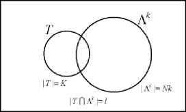
Figure 1: Venn diagram for correct and estimated support set

where (10) follows from the fact that ${\bf P}_{\Lambda^{k}}{\bf\Phi}_{T-\Lambda^{k}}{\bf x}_{T-\Lambda^{k}}\in span({\bf\Phi}_{\Lambda^{k}})$ and it can be viewed as ${\bf\Phi}_{\Lambda^{k}}{\bf z}_{\Lambda^{k}}$ where ${\bf z}_{\Lambda^{k}}\in\mathbb{R}^{\Lambda^{k}}$ and ${\bf z}_{\Lambda^{k}}={\bf\Phi}^{\dagger}_{\Lambda^{k}}{\bf\Phi}_{T-\Lambda^{k}}{\bf x}_{T-\Lambda^{k}}$. So ${\bf x}^{\prime\prime}_{T\cup\Lambda^{k}}$ is a vector in $\mathbb{R}^{T\cup\Lambda^{k}}$. Observe that

$${\bf x}^{\prime\prime}_{T\cup\Lambda^{k}}=\begin{bmatrix}x_{T-\Lambda^{k}}\\ z_{\Lambda^{k}}\end{bmatrix}$$ (12)

Let W be the set of remaining incorrect indices over which $\alpha^{k}_{i}$’s are chosen ($W\in(T\cup\Lambda^{k})^{c}$). So,

$$\alpha^{k}_{N} =min(\langle\Phi_{i},{\bf r}^{k}\rangle)\hskip 8.53581pt(i\in W)$$

$$<\frac{\sum\alpha_{i}}{N}<\sqrt{\frac{\sum\alpha_{i}^{2}}{N}}\text{ (as }|W|=N)$$

$$=\frac{||{\bf\Phi}_{W}^{T}{\bf r}^{k}||_{2}}{\sqrt{N}}$$

$$\stackrel{{\scriptstyle(11)}}{{=}}\frac{1}{\sqrt{N}}||{\bf\Phi}_{W}^{T}{\bf\Phi}_{T\cup\Lambda^{k}}{\bf x}^{\prime\prime}_{T\cup\Lambda^{k}}||_{2}$$

$$\stackrel{{\scriptstyle L1d}}{{=}}\frac{1}{\sqrt{N}}\delta_{N+Nk+K-l}||{\bf x}^{\prime\prime}_{T\cup\Lambda^{k}}||_{2}$$

$$\stackrel{{\scriptstyle L1a}}{{<}}\frac{1}{\sqrt{N}}\delta_{NK+1}||{\bf x}^{\prime\prime}_{T\cup\Lambda^{k}}||_{2}$$ (13)

where (13) comes from the fact that $l\geq k$ and $k\leq K-1$.

Now for finding lower bound of $\beta^{k}_{1}$ in terms of $||{\bf x}^{\prime\prime}_{T\cup\Lambda^{k}}||_{2}$ we proceed in this way.

$$\beta^{k}_{1}=||{\bf\Phi}_{T}^{T}{\bf r}^{k}||_{\infty}$$

$$>\frac{1}{\sqrt{K}}||{\bf\Phi}^{T}_{T}{\bf r}^{k}||_{2}\hskip 11.38109pt(as|T|=K)$$

$$=\frac{1}{\sqrt{K}}||\begin{bmatrix}{\bf\Phi}_{T}&{\bf\Phi}_{\Lambda^{k}-T}\end{bmatrix}^{T}{\bf r}^{k}||_{2}$$ (14)

$$=\frac{1}{\sqrt{K}}||{\bf\Phi}^{T}_{T\cup\Lambda^{k}}{\bf\Phi}_{T\cup\Lambda^{k}}{\bf x}^{\prime\prime}_{T\cup\Lambda^{k}}||_{2}$$

$$\stackrel{{\scriptstyle L1b}}{{>}}\frac{1}{\sqrt{K}}(1-\delta_{Nk+K-l})||{\bf x}^{\prime\prime}_{T\cup\Lambda^{k}}||_{2}$$

$$\stackrel{{\scriptstyle L1a}}{{>}}\frac{1}{\sqrt{K}}(1-\delta_{NK})||{\bf x}^{\prime\prime}_{T\cup\Lambda^{k}}||_{2}$$ (15)

where (14) comes as ${\bf\Phi}^{T}_{\Lambda^{k}-T}{\bf r}^{k}=0$ which follows from (3). Now from (13) and (15) ensuring $\beta^{k}_{1}>\alpha^{k}_{N}$ gives us the result. ∎

IV Analysis in presence of noise

In case of noise we can model the measurement as ${\bf y^{\prime}}={\bf y}+{\bf n}={\bf\Phi}{\bf x}+{\bf n}$ where ${\bf n}$ is the added noise. We can show the performance of this algorithm in presence of noise in two ways. One is by finding the upper bound of reconstruction error energy $||{\bf x}-{\bf x}_{\Lambda^{k}}||_{2}$ (as presented in [1])and other is by providing a condition for exact reconstruction subject to upper bound on measurement SNR=$\frac{||{\bf y}||_{2}}{||{\bf n}||_{2}}$.

Theorem 3.

If $k=K$ forms the stopping criterion in gOMP with ${\bf\Phi}$ satisfying $\delta_{NK+K}<1$ and $\delta_{NK}<\frac{\sqrt{N}}{\sqrt{K}+2\sqrt{N}}$ then $||{\bf x}-{\bf x}_{\Lambda^{k}}||_{2}<C_{K_{1}}||{\bf n}||_{2}$ where

$C_{K_{1}}=\frac{(1-\delta_{NK})(\sqrt{N}(1+\delta_{K})+\sqrt{K(1+\delta_{N})(1+\delta_{K})})}{(\sqrt{N}-(\sqrt{K}+2\sqrt{N})\delta_{NK})\sqrt{1-\delta_{NK+K}}}+\frac{2}{\sqrt{1-\delta_{NK+K}}}$

Proof: In Appendix B

Theorem 4.

If $k=K$ forms the stopping criterion in gOMP with ${\bf\Phi}$ satisfying $\delta_{NK+K}<1$ and $\delta_{NK+1}<\frac{\sqrt{N}}{\sqrt{K}+\sqrt{N}}$ then $||{\bf x}-{\bf x}_{\Lambda^{k}}||_{2}<C_{K_{2}}||{\bf n}||_{2}$ where

$C_{K_{2}}=\frac{(\sqrt{N}(1+\delta_{K})+\sqrt{K(1+\delta_{N})(1+\delta_{K})})}{(\sqrt{N}-(\sqrt{K}+\sqrt{N})\delta_{NK+1})\sqrt{1-\delta_{NK+K}}}+\frac{2}{\sqrt{1-\delta_{NK+K}}}$

Proof: In Appendix C

The above bounds provide a estimate on upper bound on reconstruction energy. But they do not guarantee estimation of correct support set. In some cases it may happen that the reconstruction error energy is bounded but the chosen support set is completely different. This may prove expensive because in most cases knowledge of correct support set is more important than knowledge of exact value at that position. So easily verifiable bounds guaranteeing reconstruction of correct support set are necessary.

In communication we often judge the performance by the SNR of the received signal. Before applying sparse reconstruction we do not have the information of energy of vector x. But we do have knowledge of energy of clean measurement from transmitter’s end. Hence by calculating the SNR at the receiver’s end we can have an idea whether a particular algorithm can be implemented for reconstruction or not. This can be a good measure of performance analysis for reconstruction algorithms. So we present a bound on $\frac{||y||_{2}}{||n||_{2}}$ for which correct support set is estimated. Before stating the theorem let us analyse the assumption made: $|{\bf x}_{i}|>\frac{|{\bf x}_{j}|}{\gamma}\forall i,j\in T$. This implies that all non zero values of x are bounded within some ratio of the maximum. We see that the sparse systems are modelled by setting the values of elements in x below some threshold as zero. Hence this assumption can always be made. If suppose x has a non-zero value below $\frac{|x_{max}|}{\gamma}$ then it can be modelled as a $K-1$ sparse system by setting that value to zero without affecting the output much.

Theorem 5.

If measurement ${\bf y}={\bf\Phi}{\bf x}$ is corrupted with noise ${\bf n}$ then gOMP algorithm can still recover the true support of x provided $\frac{||{\bf y}||_{2}}{||{\bf n}||_{2}}>C_{K_{3}}$ where

$$C_{K_{3}}=\frac{\sqrt{K(1+\delta_{N})}+\sqrt{N(1+\delta_{K})}}{\frac{\sqrt{N}(1-\delta_{K})(1-2\delta_{NK})}{\gamma\sqrt{(1+\delta_{K})}(1-\delta_{NK})^{2}}-\sqrt{K(1+\delta_{N})}}$$

Proof.

At first let us make use of the assumption and provide a result which would be used in subsequent proof

Lemma 4.

With usual notations we see that

$$||{\bf\Phi}_{T-\Lambda^{k}}{\bf x}_{T-\Lambda^{k}}||_{2}>\sqrt{\frac{{(K-l)(1-\delta_{K})}}{{K(1+\delta_{K})}}}\frac{||{\bf\Phi}_{T}x_{T}||_{2}}{\gamma}$$

proof: In Appendix D

Let us again compute the bounds on $\alpha^{k}_{N}$ and $\beta^{k}_{1}$

$$\alpha^{k}_{N}<\frac{||{\bf\Phi}_{W}^{T}{\bf P}_{\Lambda^{k}}^{\perp}{\bf y^{\prime}}||_{2}}{\sqrt{N}}$$

$$\stackrel{{\scriptstyle L1c}}{{<}}\frac{\sqrt{1+\delta_{N}}||{\bf P}_{\Lambda^{k}}^{\perp}{\bf y^{\prime}}||_{2}}{\sqrt{N}}$$

$$<\frac{\sqrt{1+\delta_{N}}||{\bf y^{\prime}}||_{2}}{\sqrt{N}}$$

$$<\frac{\sqrt{1+\delta_{N}}(||{\bf\Phi}_{T}{\bf x_{T}}||_{2}+||{\bf n}||_{2})}{\sqrt{N}}$$ (16)

$$\beta^{k}_{1}>\frac{1}{\sqrt{K-l}}||{\bf\Phi}^{T}_{T-\Lambda^{k}}{\bf P}_{\Lambda^{k}}^{\perp}({\bf\Phi}_{T-\Lambda^{k}}{\bf x}_{T-\Lambda^{k}}+{\bf n})||_{2}$$

$$\stackrel{{\scriptstyle L1c}}{{>}}\frac{1}{\sqrt{K-l}}||{\bf\Phi}^{T}_{T-\Lambda^{k}}{\bf P}_{\Lambda^{k}}^{\perp}{\bf\Phi}_{T-\Lambda^{k}}{\bf x}_{T-\Lambda^{k}}||_{2}$$

$$-\frac{\sqrt{1+\delta_{K}}}{\sqrt{K}}||{\bf n}||_{2}$$

$$\stackrel{{\scriptstyle(7)}}{{>}}\frac{||{\bf A}_{\Lambda^{k}}{\bf x}^{\prime}||_{2}^{2}}{\sqrt{K-l}||{\bf x}_{T-\Lambda^{k}}||_{2}}-\frac{\sqrt{1+\delta_{K}}}{\sqrt{K}}||{\bf n}||_{2}$$

$$\stackrel{{\scriptstyle L3}}{{>}}\frac{(1-(\frac{\delta_{NK}}{1-\delta_{NK}})^{2})||{\bf\Phi}_{T-\Lambda^{k}}{\bf x}_{T-\Lambda^{k}}||^{2}_{2}}{\sqrt{K-l}||{\bf x}_{T-\Lambda^{k}}||_{2}}$$

$$-\frac{\sqrt{1+\delta_{K}}}{\sqrt{K}}||{\bf n}||_{2}$$

$$\stackrel{{\scriptstyle D1}}{{>}}\frac{(1-2\delta_{NK})\sqrt{1-\delta_{K}}||{\bf\Phi}_{T-\Lambda^{k}}{\bf x}_{T-\Lambda^{k}}||_{2}}{\sqrt{K-l}(1-\delta_{NK})^{2}}$$

$$-\frac{\sqrt{1+\delta_{K}}}{\sqrt{K}}||{\bf n}||_{2}$$

$$\stackrel{{\scriptstyle L4}}{{>}}\frac{(1-2\delta_{NK})(1-\delta_{K})||{\bf\Phi}_{T}{\bf x}_{T}||_{2}}{(1-\delta_{NK})^{2}\gamma\sqrt{K(1+\delta_{K})}}-\frac{\sqrt{1+\delta_{K}}}{\sqrt{K}}||{\bf n}||_{2}$$ (17)

Making $\alpha^{k}_{N}<\beta^{k}_{1}$ ( (16) $<$ (17) ) for correct choice of index we get the desired SNR bound. ∎

V Discussion

The proposed bound in Theorem 1 is better than the one from [1] because while obtaining lower bound of $\beta^{k}_{1}$ instead of applying successive inequalities we use a more direct inequality presented in Lemma 3 which leads us to a higher lower bound. This bound is also better than the bound proposed in [14] ($\delta_{NK}<\frac{\sqrt{K}}{(2+\sqrt{2})\sqrt{K}}$) for $N<1.45K$. But according to [1] gOMP performs better than OMP for small values of N only.

It is difficult to compare the bounds presented in Theorem 1 and Theorem 2 since $\delta_{NK}<\delta_{NK+1}$ and $\frac{\sqrt{N}}{\sqrt{K}+\sqrt{N}}>\frac{\sqrt{N}}{\sqrt{K}+2\sqrt{N}}$. But intuitively we can see that bound on $\delta_{NK+1}$ is more optimal since it reduces to near optimal bound on OMP for special case of $N=1$. The proposition on SNR seems to be a good approach since it is an easily measurable quantity and can be used in future research for comparing greedy algorithm’s performance under noise.

VI Conclusions

In this paper, we have given an elegent proof of the theoretical performance of gOMP algorithm. Our analysis improves the bound on RIP of order $NK$ from $\delta_{NK}<\frac{\sqrt{N}}{\sqrt{K}+3\sqrt{N}}$ [1] to $\delta_{NK}<\frac{\sqrt{N}}{\sqrt{K}+2\sqrt{N}}$. In the same paper, we have presented another bound of order $NK+1$ with RIP constant $\delta_{NK+1}<\frac{\sqrt{N}}{\sqrt{K}+\sqrt{N}}$. We have also presented improved theoretical performance of gOMP algorithm under noisy measurements.

Appendix A Proof of lemma 3

We know that

$$||{\bf\Phi}{\bf u}||_{2}^{2}=||{\bf P}_{I_{1}}{\bf\Phi}{\bf u}||_{2}^{2}+||{\bf P}_{I_{1}}^{\perp}{\bf\Phi}{\bf u}||_{2}^{2}$$

$$\Rightarrow ||{\bf A}_{I_{1}}{\bf u}||_{2}^{2}=||{\bf\Phi}{\bf u}||_{2}^{2}-||{\bf P}_{I_{1}}{\bf\Phi}{\bf u}||_{2}^{2}$$ (A.1)

Now $\langle{\bf P}_{I_{1}}{\bf\Phi}{\bf u},{\bf\Phi}{\bf u}\rangle=({\bf\Phi}{\bf u})^{T}{\bf P}_{I_{1}}^{T}{\bf\Phi}{\bf u}=({\bf\Phi}{\bf u})^{T}{\bf P}_{I_{1}}^{T}{\bf P}_{I_{1}}{\bf\Phi}{\bf u}=||{\bf P}_{I_{1}}{\bf\Phi}{\bf u}||_{2}^{2}$. Further we see that ${\bf P}_{I_{1}}{\bf\Phi}{\bf u}\in span({\bf\Phi}_{I_{1}})$. So ${\bf P}_{I_{1}}{\bf\Phi}{\bf u}={\bf\Phi}{\bf z}$ for some ${\bf z}\in\mathbb{R}^{n}$ with $supp({\bf z})\in{I_{1}}$.

$$\frac{||{\bf P}_{I_{1}}{\bf\Phi}{\bf u}||_{2}}{||{\bf\Phi}{\bf u}||_{2}}=\frac{\langle{\bf P}_{I_{1}}{\bf\Phi}{\bf u},{\bf\Phi}{\bf u}\rangle}{||{\bf P}_{I_{1}}{\bf\Phi}{\bf u}||_{2}||{\bf\Phi}{\bf u}||_{2}}=\frac{\langle{\bf\Phi}{\bf z},{\bf\Phi}{\bf u}\rangle}{||{\bf\Phi}{\bf z}||_{2}||{\bf\Phi}{\bf u}||_{2}}$$

$$\stackrel{{\scriptstyle D1,L1d}}{{<}}\frac{\delta_{|I_{1}|+|I_{2}|}}{\sqrt{1-\delta_{|I_{1}|}}\sqrt{1-\delta_{|I_{2}|}}}$$

$$\stackrel{{\scriptstyle L1a}}{{<}}\frac{\delta_{|I_{1}|+|I_{2}|}}{1-\delta_{|I_{1}|+|I_{2}|}}$$ (A.2)

So from (A.1) and (A.2) we get$||{\bf A}_{I_{1}}{\bf u}||_{2}^{2}>(1-(\dfrac{\delta_{|I_{1}|+|I_{2}|}}{1-\delta_{|I_{1}|+|I_{2}|}})^{2})||{\bf\Phi}{\bf u}||_{2}^{2}>(1-(\dfrac{\delta_{|I_{1}|+|I_{2}|}}{1-\delta_{|I_{1}|+|I_{2}|}})^{2})(1-\delta_{|I_{2}|})||{\bf u}||_{2}^{2}\stackrel{{\scriptstyle L1a}}{{>}}(1-\dfrac{\delta_{|I_{1}|+|I_{2}|}}{1-\delta_{|I_{1}|+|I_{2}|}})||{\bf u}||_{2}^{2}$. Applying $||{\bf P}_{I_{1}}{\bf\Phi}{\bf u}||_{2}^{2}>0$ in (A.1) the upper bound becomes$||{\bf A}_{I_{1}}{\bf u}||_{2}^{2}<||{\bf\Phi}{\bf u}||_{2}^{2}<(1+\delta_{|I_{2}|})||{\bf u}||_{2}^{2}\stackrel{{\scriptstyle L1a}}{{<}}(1+\delta_{|I_{1}|+|I_{2}|})||{\bf u}||_{2}$.

Appendix B Proof of theorem 3

First we need to find the bounds on $\alpha^{k}_{N}$ and $\beta^{k}_{1}$ in presence of noise in k+1^th iteration

$$\alpha^{k}_{N}<\frac{||{\bf\Phi}_{W}^{T}{\bf r}^{k}||_{2}}{\sqrt{N}}$$

$$=\frac{1}{\sqrt{N}}||{\bf\Phi}_{W}^{T}({\bf P}^{\perp}_{\Lambda^{k}}{\bf y}+{\bf P}^{\perp}_{\Lambda^{k}}{\bf n})||_{2}$$

$$<\frac{1}{\sqrt{N}}(||{\bf\Phi}_{W}^{T}P^{\perp}_{\Lambda^{k}}{\bf y}||_{2}+||{\bf\Phi}_{W}^{T}P^{\perp}_{\Lambda^{k}}{\bf n}||_{2})$$

$$\stackrel{{\scriptstyle L2,L1c}}{{<}}\frac{1}{\sqrt{N}}\frac{\delta_{NK}}{1-\delta_{NK}}||{\bf x}_{T-\Lambda^{k}}||_{2}+\frac{\sqrt{1+\delta_{N}}}{\sqrt{N}}||{\bf P}^{\perp}_{\Lambda^{k}}{\bf n}||_{2}$$

$$<\frac{1}{\sqrt{N}}\frac{\delta_{NK}}{1-\delta_{NK}}||{\bf x}_{T-\Lambda^{k}}||_{2}+\frac{\sqrt{1+\delta_{N}}}{\sqrt{N}}||{\bf n}||_{2}$$ (B.1)

and

$$\beta^{k}_{1}>\frac{1}{\sqrt{K}}||{\bf\Phi}^{T}_{T-\Lambda^{k}}{\bf P}_{\Lambda^{k}}^{\perp}{\bf y^{\prime}}||_{2}$$

$$>\frac{1}{\sqrt{K}}||{\bf\Phi}^{T}_{T-\Lambda^{k}}{\bf P}_{\Lambda^{k}}^{\perp}{\bf\Phi}_{T}{\bf x}_{T}||_{2}-\frac{1}{\sqrt{K}}||{\bf\Phi}^{T}_{T-\Lambda^{k}}{\bf P}_{\Lambda^{k}}^{\perp}{\bf n}||_{2}$$

$$\stackrel{{\scriptstyle(9),L1c}}{{>}}\frac{1}{\sqrt{K}}(1-\frac{\delta_{NK}}{1-\delta_{NK}})||{\bf x}_{T-\Lambda^{k}}||_{2}-\frac{\sqrt{1+\delta_{K}}}{\sqrt{K}}||{\bf P}_{\Lambda^{k}}^{\perp}{\bf n}||_{2}$$

$$>\frac{1}{\sqrt{K}}(1-\frac{\delta_{NK}}{1-\delta_{NK}})||{\bf x}_{T-\Lambda^{k}}||_{2}-\frac{\sqrt{1+\delta_{K}}}{\sqrt{K}}||{\bf n}||_{2}$$ (B.2)

Now at the end of algorithm it may happen that some incorrect atoms are chosen. Lets say this happens for the first time in the p+1^th step. Then at this particular step (B.1)$>$(B.2). Which implies

$$||{\bf x}_{T-\Lambda^{p}}||_{2}< \frac{(1-\delta_{NK})(\sqrt{N(1+\delta_{K})}+\sqrt{K(1+\delta_{N})})}{(\sqrt{N}-(\sqrt{K}+2\sqrt{N})\delta_{NK})}$$

$$\times||{\bf n}||_{2}$$ (B.3)

The error in reconstruction energy can be seen as

$$||{\bf x}-{\bf x}_{\Lambda^{K}}||_{2}\stackrel{{\scriptstyle D1}}{{<}}\frac{||{\bf\Phi}{\bf x}-{\bf\Phi}{\bf x}_{\Lambda^{K}}||_{2}}{\sqrt{1-\delta_{NK+K}}}$$

$$=\frac{||{\bf\Phi}{\bf x}-{\bf\Phi}{\bf\Phi}^{\dagger}_{\Lambda^{K}}{\bf y^{\prime}}||_{2}}{\sqrt{1-\delta_{NK+K}}}$$

$$=\frac{||{\bf y^{\prime}}-{\bf P}_{\Lambda^{K}}{\bf y^{\prime}}-{\bf n}||_{2}}{\sqrt{1-\delta_{NK+K}}}$$

$$<\frac{||{\bf P}^{\perp}_{\Lambda^{K}}{\bf y^{\prime}}||_{2}+||{\bf n}||_{2}}{\sqrt{1-\delta_{NK+K}}}$$

$$=\frac{||{\bf r}^{K}||_{2}+||{\bf n}||_{2}}{\sqrt{1-\delta_{NK+K}}}$$

$$\leq\frac{||{\bf r}^{p}||_{2}+||{\bf n}||_{2}}{\sqrt{1-\delta_{NK+K}}}(\text{as }||{\bf r}^{i}||_{2}\leq||{\bf r}^{j}||_{2}\text{ for }i>j)$$

$$=\frac{||{\bf P}^{\perp}_{\Lambda^{p}}({\bf\Phi}_{T}{\bf x}_{T}+{\bf n})||_{2}+||{\bf n}||_{2}}{\sqrt{1-\delta_{NK+K}}}$$

$$<\frac{||{\bf P}^{\perp}_{\Lambda^{p}}{\bf\Phi}_{T}{\bf x}_{T}||_{2}+||{\bf P}^{\perp}_{\Lambda^{p}}{\bf n}||_{2}+||{\bf n}||_{2}}{\sqrt{1-\delta_{NK+K}}}$$

$$<\frac{||{\bf P}^{\perp}_{\Lambda^{p}}{\bf\Phi}_{T-\Lambda^{p}}{\bf x}_{T-\Lambda^{p}}||_{2}+2||{\bf n}||_{2}}{\sqrt{1-\delta_{NK+K}}}$$

$$<\frac{||{\bf\Phi}_{T-\Lambda^{p}}{\bf x}_{T-\Lambda^{p}}||_{2}+2||{\bf n}||_{2}}{\sqrt{1-\delta_{NK+K}}}$$

$$\stackrel{{\scriptstyle D1}}{{<}}\frac{\sqrt{1+\delta_{K}}||{\bf x}_{T-\Lambda^{p}}||_{2}+2||{\bf n}||_{2}}{\sqrt{1-\delta_{NK+K}}}$$ (B.4)

By using (B.3) in (B.4) we get the desired bound.

Appendix C Proof of theorem 4

In this case we find the bounds on $\alpha^{k}_{N}$ and $\beta^{k}_{1}$ in presence of noise similar to our proof on second bound of gOMP. Proceding similar to (B.1) and (B.2) we get

$$\alpha^{k}_{N}<\frac{1}{\sqrt{N}}\delta_{NK+1}||{\bf x}^{\prime\prime}_{T\cup\Lambda^{k}}||_{2}+\frac{\sqrt{1+\delta_{N}}}{\sqrt{N}}||{\bf n}||_{2}$$ (C.1)

$$\beta^{k}_{1}>\frac{1-\delta_{NK}}{\sqrt{K}}||{\bf x}^{\prime\prime}_{T\cup\Lambda^{k}}||_{2}-\frac{\sqrt{1+\delta_{K}}}{\sqrt{K}}||{\bf n}||_{2}$$ (C.2)

So failure at p+1^th step implies

$$||{\bf x}^{\prime\prime}_{T\cup\Lambda^{p}}||_{2}<\frac{\sqrt{N(1+\delta_{K})}+\sqrt{K(1+\delta_{N})}}{(\sqrt{N}-(\sqrt{K}+\sqrt{N})\delta_{NK+1})}||n||_{2}$$ (C.3)

Now to get an upper bound in estimation error we proceed similarly as in (B.4)

$$||{\bf x}-{\bf x}_{\Lambda^{K}}||_{2}<\frac{\sqrt{1+\delta_{K}}||{\bf x}_{T-\Lambda^{p}}||_{2}+2||{\bf n}||_{2}}{\sqrt{1-\delta_{NK+K}}}$$

$$\stackrel{{\scriptstyle(12)}}{{<}}\frac{\sqrt{1+\delta_{K}}||{\bf x}^{\prime\prime}_{T\cup\Lambda^{p}}||_{2}+2||{\bf n}||_{2}}{\sqrt{1-\delta_{NK+K}}}$$

$$\stackrel{{\scriptstyle(C.3)}}{{<}}C_{K_{2}}||{\bf n}||_{2}$$ (C.4)

Appendix D Proof of Lemma 4

$$||{\bf\Phi}_{T-\Lambda^{k}}{\bf x}_{T-\Lambda^{k}}||_{2}\stackrel{{\scriptstyle D1}}{{>}}\sqrt{1-\delta_{K}}||{\bf x}_{T-\Lambda^{k}}||_{2}$$

$$>\sqrt{(1-\delta_{K})(K-l)}|{\bf x}_{min}|$$

$$>\sqrt{\frac{(1-\delta_{K})(K-l)}{K}}\frac{||{\bf x}_{T}||_{2}}{\gamma}$$

$$\stackrel{{\scriptstyle D1}}{{>}}\sqrt{\frac{(1-\delta_{K})(K-l)}{K(1+\delta_{K})}}\frac{||{\bf\Phi}_{T}x_{T}||_{2}}{\gamma}$$ (D.1)

References

- [1] J. Wang, S. Kwon, and B. Shim, “Generalized orthogonal matching pursuit,” IEEE Trans. on Signal Processing, vol. 60, no. 12, pp. 6202–6216, dec. 2012.
- [2] J. Wang and B. Shim, “On the recovery limit of sparse signals using orthogonal matching pursuit,” IEEE Trans. on Signal Processing, vol. 60, no. 9, pp. 4973–4976, sept. 2012.
- [3] D. Donoho, “Compressed sensing,” IEEE Trans. on Information Theory, vol. 52, no. 4, pp. 1289–1306, Apr. 2006.
- [4] E. Candes, “Compressive sampling,” in Int. Congress of Mathematics, vol. 3, 2006, pp. 1433–1452.
- [5] R. Baraniuk, “Compressed sensing,” IEEE Signal Processing Magazine, vol. 25, pp. 21–30, 2007.
- [6] S. Chen and D. Donoho, “Basis pursuit,” in Proc. 28th Asilomar Conf. Signals, Syst. Comput., 1994, pp. 41–44.
- [7] S. S. Chen, D. L. Donoho, and M. A. Saunders, “Atomic decomposition by basis pursuit,” SIAM J. Scientif. Comput., vol. 20, no. 1, pp. 33–61, 1998.
- [8] R. Tibshirani, “Regression shrinkage and selection via the lasso,” J. Royal. Statist. Soc B., vol. 58, pp. 267–288, 1996.
- [9] J. R. E. Candès and T. Tao, “Robust uncertainty principles: exact signal reconstruction from highly incomplete frequency information,” IEEE Trans. on Inf. Theory, vol. 52, no. 2, pp. 489–509, Feb. 2006.
- [10] E. J. Candès, “The restricted isometry property and its implications for compressed sensing,” in Compte Rendus de l’Academie des Sciences, ser. I, no. 346, 2008, pp. 589–592.
- [11] G. X. J. Z. T. Tony Cai, “On recovery of sparse signals via minimization,” IEEE Trans. on Inf. Theory, vol. 55, no. 7, pp. 3388–3397, 2009.
- [12] S. Foucart, “A note on guaranteed sparse recovery via -minimization,” Appl. Comput. Harmon.Anal., vol. 29, no. 1, pp. 97–103, 2010.
- [13] J.A. Tropp and A. Gilbert, “Signal recovery from random measurements via orthogonal matching pursuit,” IEEE Trans. on Info. Theory, vol. 53, no. 12, pp. 4655–4666, 2007.
- [14] E. Liu and V. N. Temlyakov, “The orthogonal super greedy algorithm and applications in compressed sensing,” Inverse Problem, vol. 58, no. 4, pp. 2040–2047, 2012.
- [15] S. A. B. S. Chen and W. . Luo, “Orthogonal least squares methods and their application to non-linear system identification,” Int. J. Contr., vol. 50, no. 5, pp. 1873–1896, 1989.
- [16] D. Needell and J. Tropp, “Cosamp : Iterative signal recovery from incomplete and inaccurate samples,” Appl. Comput. Harmon. Anal., vol. 26, pp. 301–321, 2009.
- [17] W. Dai and O. Milenkovic, “Subspace pursuit for compressive sensing signal reconstruction,” IEEE Trans. on Inf. Theory, vol. 55, no. 5, pp. 2230–2249, 2009.
- [18] M. A. Davenport and M. B. Wakin, “Analysis of orthogonal matching pursuit using the restricted isometry property,” IEEE Trans. on Information Theory, vol. 56, no. 9, pp. 4395–4401, 2010.
- [19] S. Huang and J. Zhu, “Recovery of sparse signals using OMP and its variants: Convergence analysis based on RIP,” Inverse Problem, vol. 27, no. 3, 2011.
- [20] Q. Mo and Y. Shen, “A remark on the restricted isometry property in orthogonal matching pursuit,” Information Theory, IEEE Transactions on, vol. 58, no. 6, pp. 3654 –3656, june 2012.