Low-Complexity Reduced-Rank Beamforming Algorithms

Abstract

A reduced-rank framework with set-membership filtering (SMF) techniques is presented for adaptive beamforming problems encountered in radar systems. We develop and analyze stochastic gradient (SG) and recursive least squares (RLS)-type adaptive algorithms, which achieve an enhanced convergence and tracking performance with low computational cost as compared to existing techniques. Simulations show that the proposed algorithms have a superior performance to prior methods, while the complexity is lower.

I Introduction

With the development of array signal processing techniques, beamforming has long been investigated for numerous applications in radar, sonar, seismology, and wireless communications [2], [3]. The most well-known beamforming technique is the optimal linearly constrained minimum variance (LCMV) beamformer [4, 5]. It exploits the second-order statistics of the received vector to minimize the array output power while constraining the array response in the direction of the signal of interest (SOI) to be constant. In general, the constraint corresponds to prior knowledge of the direction of arrival (DOA) of the SOI.

Many adaptive algorithms have been reported for the implementation of the LCMV beamformer, ranging from the low-complexity stochastic gradient (SG) algorithm to the more complex recursive least squares (RLS) algorithm [6]. According to the parameter estimation strategy of the algorithm, the SG and RLS algorithms can be included in the class of full-rank processing techniques[12]. The full-rank adaptive algorithms usually require a large number of snapshots to reach the steady-state when the number of elements in the beamformer is large, and the resulting convergence speed reduces significantly. In dynamic scenarios (e.g., when interferers enter or exit a given system), filters with many elements show a poor tracking performance when dealing with signals embedded in interference and noise. These situations are quite relevant in defence systems such as radar. Other strategies for interference suppression coming from the antenna community include the recent work by Massa et al. [7] that introduces a dynamic thinning strategy, the work by D’Urso et al. [8] that considers a hybrid optimization procedure that adjusts both clustering into subarrays and excitations of the subarrays, the contribution of Haupt [9] which uses subarrays a hybrid genetic algorithm to optimize the size of the subarrays their weights, the method of Haupt and Aten [10] which employs a genetic algorithm to optimize the orientation of each dipole in an array, and the technique by Haupt et al. [11] that uses partial adaptation of the beamforming weights.

These problems motivate us to investigate a more effective signal processing approach known as reduced-rank signal processing, which allows a designer to address the drawbacks of full-rank algorithms. The idea is to employ a transformation matrix that projects the received signal onto a lower dimensional subspace, and then the reduced-rank filter optimization occurs within this subspace. This has the advantage of improving the convergence and tracking performance. The advantage is more obvious when the number of sensor elements in the array is large. Well-known reduced-rank schemes include the multistage Wiener filter (MSWF) [13]-[16], the auxiliary vector filtering (AVF) [17],[18] the joint iterative optimization (JIO) [19]-[23] and the joint interpolation, decimation and filtering (JIDF)-based approaches [24]-[26]. They employ different procedures to construct the transformation matrix and to estimate the parameters. A common problem of these reduced-rank schemes is the relatively high computational load required to compute the transformation matrix.

An efficient approach to reducing the computational complexity is to employ a set-membership filtering (SMF) technique [27, 28] for the beamformer design. The SMF specifies a predetermined bound on the magnitude of the estimation error or the array output and performs data-selective updates to estimate the parameters. It involves two steps: $1)$ information evaluation (depending on the predetermined bound) and $2)$ parameter update (depending on step $1)$). If the parameter update does not occur frequently, and the information evaluation does not require much complexity, the overall complexity can be substantially reduced. The well-known SMF algorithms include the SG-based algorithms in [27] and the RLS-based algorithms in [28], [29]. These algorithms are examples of the application of the SMF technique in the full-rank signal processing context.

The objective of this paper is to introduce a constrained reduced-rank framework and algorithms for achieving a superior convergence and tracking performance with significantly lower computational cost comparable with their reduced-rank counterparts. We consider reduced-rank LCMV designs using the SMF concept that imposes a bounded constraint on the array output and the JIO strategy. The joint optimization of the transformation matrix and the reduced-rank filter are then performed for beamforming. The reduced-rank parameters only update if the bounded constraint cannot be satisfied. This partial update plays a positive role in increasing the convergence speed. The updated parameters belong to a set of feasible solutions. Considering the fact that the predetermined bound degrades the performance of the SMF technique due to the lack of knowledge of the environment, we utilize a parameter-dependent time-varying bound instead to guarantee a good performance. Related work can be found in [30], [31] but only focuses on the full-rank signal processing context. In this paper, we introduce this technique into the reduced-rank signal processing context. The proposed framework, referred here as JIO-SM, inherits the positive features of the reduced-rank JIO schemes that jointly and iteratively exchange information between the transformation matrix and the reduced-rank filter, and performs beamforming using the SMF data-selective updates. We propose constrained reduced-rank SG-based and RLS-based adaptive algorithms, namely, JIO-SM-SG and JIO-SM-RLS, for the design of the proposed beamformer. A discussion on the properties of the developed algorithms is provided. Specifically, a complexity comparison is presented to show the advantages of the proposed algorithms over their existing counterparts. A mean-squared error (MSE) expression to predict the performance of the proposed JIO-SM-SG algorithm is derived. We also analyze the properties of the optimization problem by employing the SMF constraint. Simulations are provided to show the performance of the proposed and existing algorithms.

The remainder of this paper is organized as follows: we outline a system model for beamforming in Section II. Based on this model, the full-rank and the reduced-rank LCMV beamformer are reviewed. The novel reduced-rank framework based on the JIO scheme and the SMF technique is presented in Section III, and the proposed adaptive algorithms are detailed in Section IV. A complexity study and the related analyses of the proposed algorithms are carried out in Section V. Simulation results are provided and discussed in Section VI, and conclusions are drawn in Section VII.

II System Model and LCMV Beamformer Design

In this section, we describe a system model to express the array received vector. Based on this model, the full-rank and the reduced-rank LCMV beamformers are introduced.

II-A System Model

Let us suppose that $q$ narrowband signals impinge on a uniform linear array (ULA) of $m$ ($m\geq q$) sensor elements. The sources are assumed to be in the far field with DOAs $\theta_{0}$,…,$\theta_{q-1}$. The received vector $\boldsymbol{x}\in\mathbb{C}^{m\times 1}$ can be modeled as

$$\centering{\boldsymbol{x}}={\boldsymbol{A}}({\boldsymbol{\theta}}){\boldsymbol{s}}+{\boldsymbol{n}},\@add@centering$$ (1)

where $\boldsymbol{\theta}=[\theta_{0},\ldots,\theta_{q-1}]^{T}\in{\mathbb{R}}^{q\times 1}$ is the vector with the signals’ DOAs, ${\boldsymbol{A}}({\boldsymbol{\theta}})=[{\boldsymbol{a}}(\theta_{0}),\ldots,{\boldsymbol{a}}(\theta_{q-1})]\in\mathbb{C}^{m\times q}$ comprises the normalized signal steering vectors ${\boldsymbol{a}}(\theta_{k})=[1,e^{-2\pi j\frac{u}{\lambda_{\textrm{c}}}cos{\theta_{k}}},\ldots$, $e^{-2\pi j(m-1)\frac{u}{\lambda_{\textrm{c}}}cos{\theta_{k}}}]^{T}\in\mathbb{C}^{m\times 1}$, $(k=0,\ldots,q-1)$, where $\lambda_{\textrm{c}}$ is the wavelength and $u$ ($u=\lambda_{\textrm{c}}/2$ in general) is the inter-element distance of the ULA. To avoid mathematical ambiguities, the steering vectors $\boldsymbol{a}(\theta_{k})$ are assumed to be linearly independent, ${\boldsymbol{s}}\in\mathbb{C}^{q\times 1}$ is the source data vector, ${\boldsymbol{n}}\in\mathbb{C}^{m\times 1}$ is the noise vector, which is assumed to be a zero-mean spatially and Gaussian process, and $(\cdot)^{T}$ stands for transpose.

II-B Full-rank LCMV Beamformer Design

The full-rank LCMV beamformer design is equivalent to determining a set of filter parameters $\boldsymbol{w}=[w_{1},\ldots,w_{m}]^{T}\in\mathbb{C}^{m\times 1}$ that provide the array output $y=\boldsymbol{w}^{H}\boldsymbol{x}$, where $(\cdot)^{H}$ represents Hermitian transpose. The filter parameters are calculated by solving the following optimization problem:

$$\textrm{minimize}~{}~{}\mathbb{E}[|y|^{2}]=\mathbb{E}[|\boldsymbol{w}^{H}\boldsymbol{x}|^{2}],~{}~{}~{}~{}~{}\textrm{subject~{}to}~{}~{}\boldsymbol{w}^{H}\boldsymbol{a}(\theta_{0})=\gamma,$$ (2)

where $\boldsymbol{a}(\theta_{0})$ is the full-rank steering vector of the SOI and $\gamma$ is a constant. The objective of (2) is to minimize the array output power while maintaining the contribution from $\theta_{0}$ constant.

The solution of the LCMV optimization problem is

$$\boldsymbol{w}_{\textrm{opt}}=\frac{\gamma\boldsymbol{R}^{-1}\boldsymbol{a}(\theta_{0})}{\boldsymbol{a}^{H}(\theta_{0})\boldsymbol{R}^{-1}\boldsymbol{a}(\theta_{0})},$$ (3)

where $\boldsymbol{R}=\mathbb{E}[\boldsymbol{x}\boldsymbol{x}^{H}]\in\mathbb{C}^{m\times m}$ is the received data covariance matrix. The filter $\boldsymbol{w}$ can be estimated in an adaptive way via SG or RLS algorithms, where $\boldsymbol{R}$ is calculated by its sample estimate. However, their convergence and tracking performance depends on the filter length $m$, and degrades when $m$ is large [6], [21].

II-C Reduced-rank LCMV Beamformer Design

An important feature of the reduced-rank schemes is to construct a transformation matrix $\boldsymbol{T}_{r}\in\mathbb{C}^{m\times r}$ that performs the dimensionality reduction that projects the full-rank received vector onto a lower dimension, which is given by

$$\bar{\boldsymbol{x}}=\boldsymbol{T}_{r}^{H}\boldsymbol{x},$$ (4)

where $\bar{\boldsymbol{x}}$ denotes the reduced-rank received vector and $r(1\leq r\leq m)$ is the rank. In what follows, all $r$-dimensional quantities are denoted with a “bar”.

The reduced-rank LCMV beamformer estimates the parameters $\bar{\boldsymbol{w}}=[\bar{w}_{1},\ldots,\bar{w}_{r}]^{T}\in\mathbb{C}^{r\times 1}$ to generate the array output $y=\bar{\boldsymbol{w}}^{H}\bar{\boldsymbol{x}}$. The reduced-rank filter is designed by solving the optimization problem:

$$\begin{split}\textrm{minimize}~{}~{}\mathbb{E}[|y|^{2}]&=\mathbb{E}[|\bar{\boldsymbol{w}}^{H}\bar{\boldsymbol{x}}|^{2}],\\ \textrm{subject~{}to}~{}~{}\bar{\boldsymbol{w}}^{H}\bar{\boldsymbol{a}}(\theta_{0})&=\gamma,\end{split}$$ (5)

where $\bar{\boldsymbol{a}}(\theta_{0})=\boldsymbol{T}_{r}^{H}\boldsymbol{a}(\theta_{0})$ is the reduced-rank steering vector with respect to the SOI. The solution of the reduced-rank LCMV optimization problem is

$$\begin{split}\bar{\boldsymbol{w}}_{\textrm{opt}}=\frac{\gamma\bar{\boldsymbol{R}}^{-1}\bar{\boldsymbol{a}}(\theta_{0})}{\bar{\boldsymbol{a}}^{H}(\theta_{0})\bar{\boldsymbol{R}}^{-1}\bar{\boldsymbol{a}}(\theta_{0})},\end{split}$$ (6)

where $\bar{\boldsymbol{R}}=\mathbb{E}[\bar{\boldsymbol{x}}\bar{\boldsymbol{x}}^{H}]=\boldsymbol{T}_{r}^{H}\boldsymbol{R}\boldsymbol{T}_{r}\in\mathbb{C}^{r\times r}$ is the reduced-rank data covariance matrix. The MSWF [15], [16], the AVF [17], and the JIO [19] are effective reduced-rank schemes to construct the transformation matrix aided by SG-based or RLS-based adaptive algorithms for parameter estimation. However, there is a number of problems and limitations with the existing techniques. The computational complexity of algorithms dealing with a large number of parameters can be substantial. It is difficult to predetermine the step size or the forgetting factor values to achieve a satisfactory tradeoff between fast convergence and misadjustment [3]. The RLS algorithm present problems with numerical stability and divergence [6]. Furthermore, the computational cost is high if the transformation matrix has to be updated for each snapshot.

III Proposed JIO-SM Framework

In order to address some of the problems stated in Section II, we introduce a new constrained reduced-rank framework to address them by combining the SMF techniques with the reduced-rank JIO scheme, as depicted in Fig. 1. In this structure, the transformation matrix is constructed using a bank of $r$ full-rank filters $\boldsymbol{t}_{j}=[t_{1,j},t_{2,j},\ldots,t_{m,j}]^{T}\in\mathbb{C}^{m\times 1}$, ($j=1,\ldots,r$), as given by $\boldsymbol{T}_{r}=[\boldsymbol{t}_{1},\boldsymbol{t}_{2},\ldots,\boldsymbol{t}_{r}]$. The transformation matrix processes the received vector $\boldsymbol{x}$ for reducing the dimension, and retains the key information of the original signal in the generated reduced-rank received vector $\bar{\boldsymbol{x}}$. The reduced-rank filter $\bar{\boldsymbol{w}}$ then computes the output $y$.

Figure 1: Proposed reduced-rank JIO-SM structure.

For the JIO scheme, the reduced-rank adaptive algorithms [19] are developed to update $\boldsymbol{T}_{r}$ and $\bar{\boldsymbol{w}}$ with respect to each time instant “$i$”. In the proposed JIO-SM structure, the SMF check is embedded to specify a time-varying bound $\delta$ (with respect to $i$) on the amplitude of the array output $y$. The time-varying bound is related to the previous transformation matrix and the reduced-rank weight vector. The parameter update is only performed if the constraint on the bound $|y|^{2}\leq|\delta|^{2}$ cannot be satisfied. At each time instant, some valid pairs $\{\boldsymbol{T}_{r},\bar{\boldsymbol{w}}\}$ are consistent with the bound. Therefore, the solution to the proposed JIO-SM scheme is a set in the parameter space. Some pairs of $\{\boldsymbol{T}_{r},\bar{\boldsymbol{w}}\}$ even satisfy the constrained condition with respect to different received vectors for different “$i$”. Thus, the proposed scheme only takes the data-selective updates and ensures all the updated pairs satisfy the constraint for the current time instant. In comparison, the conventional full-rank or reduced-rank filtering schemes only provide a point estimate with respect to the received vector for each time instant. This estimate may not satisfy the condition with respect to other received vectors (at least before the algorithm achieves the steady-state). Compared with the existing SMF techniques [27]-[29], the proposed scheme takes both $\boldsymbol{T}_{r}$ and $\bar{\boldsymbol{w}}$ into consideration with respect to the bounded constraint in order to promote an exchange of information between them. This procedure ensures the key information of the original signal to be utilized more effectively.

Let $\mathcal{H}_{i}$ denote the set containing all the pairs of $\{\boldsymbol{T}_{r},\bar{\boldsymbol{w}}\}$ for which the associated array output at time instant $i$ is upper bounded in magnitude by $\delta$, which is

$$\mathcal{H}_{i}=\big{\{}\boldsymbol{T}_{r}\in\mathbb{C}^{m\times r},\bar{\boldsymbol{w}}\in\mathbb{C}^{r\times 1}:~{}|y|^{2}\leq\delta^{2}\big{\}},$$ (7)

where $\mathcal{H}_{i}$ is bounded by a set of hyperplanes that correspond to the pairs of $\{\boldsymbol{T}_{r},\bar{\boldsymbol{w}}\}$. The set $\mathcal{H}_{i}$ is referred to as the constraint set. We then define the exact feasibility set $\Theta_{i}$ as the intersection of the constraint sets over the time instants $l=1,\ldots,i$, which is given by

$$\Theta_{i}={\bigcap_{l=1}^{i}}_{(s_{0},\boldsymbol{x})\in{\boldsymbol{S}}}\mathcal{H}_{l},$$ (8)

where $s_{0}$ is the SOI and $\boldsymbol{S}$ is the set including all possible data pairs $\{s_{0},\boldsymbol{x}\}$. The aim of (8) is to develop adaptive algorithms that update the parameters such that they will always remain within the feasibility set. In theory, $\Theta$ should encompass all the pairs of solutions $\{\boldsymbol{T}_{r},\bar{\boldsymbol{w}}\}$ that satisfy the bounded constraint until $i\rightarrow\infty$. In practice, $\boldsymbol{S}$ cannot be traversed all over. It implies that a larger space of the data pairs provided by the observations leads to a smaller feasibility set. Thus, as the number of data pairs (or “$i$”) increases, there are fewer pairs of $\{\boldsymbol{T}_{r},\bar{\boldsymbol{w}}\}$ that can be found to satisfy the constraint. Under this condition, we define the membership set $\Psi_{i}=\bigcap_{l=1}^{i}\mathcal{H}_{l}$ as the practical set of the proposed JIO-SM scheme. It is obvious that $\Theta$ is a limiting set of $\Psi$. These two sets will be equal if the data pairs traverse $\boldsymbol{S}$ completely.

The proposed JIO-SM framework introduces the principle of the SMF technique into the constrained reduced-rank signal processing for reducing the computational complexity. The reduced number of parameters and data-selective updates reduce the complexity. It should be remarked that, due to the time-varying nature of many practical environments, the time-varying bound should be selected appropriately to account for the characteristics of the environment. Moreover, the use of an appropriate bound will lead to highly effective variable step-sizes and forgetting factors for the SG-based and RLS-based algorithms, respectively, an increased convergence speed and improved tracking ability. We will detail their relations next.

IV Proposed JIO-SM Adaptive Algorithms

We derive SG-based and RLS-based adaptive algorithms for the proposed JIO-SM scheme. They are developed according to the reduced-rank LCMV optimization problem that incorporates the time-varying bounded constraint on the amplitude of the array output. The problem is defined as:

$$\begin{split}&\textrm{minimize}~{}~{}~{}\mathbb{E}[|\bar{\boldsymbol{w}}^{H}\boldsymbol{T}_{r}^{H}\boldsymbol{x}|^{2}]=\bar{\boldsymbol{w}}^{H}\bar{\boldsymbol{R}}\bar{\boldsymbol{w}}\\ &\textrm{subject~{}to}~{}~{}~{}\bar{\boldsymbol{w}}^{H}\bar{\boldsymbol{a}}(\theta_{0})=\gamma~{}\textrm{and}~{}|\bar{\boldsymbol{w}}^{H}\boldsymbol{T}_{r}^{H}\boldsymbol{x}|^{2}=\delta^{2},\end{split}$$ (9)

The optimization problem in (9) is a function of $\boldsymbol{T}_{r}$ and $\bar{\boldsymbol{w}}$. In order to obtain a solution, we employ an alternating optimization strategy, which is equivalent to fixing $\bar{\boldsymbol{w}}$ and computing $\boldsymbol{T}_{r}$ with a suitable adaptive algorithm followed by another step with $\boldsymbol{T}_{r}$ fixed and the use of another adaptive algorithm to adjust $\bar{\boldsymbol{w}}$. This will be pursued in what follows with constrained SG and RLS-type algorithms for which a time-varying bound $\delta[i]$ determines a set of solutions $\{\boldsymbol{T}_{r},\bar{\boldsymbol{w}}\}$ within the constraint set $\mathcal{H}$ at each time instant. Regarding the convergence of this type of strategy, a general alternating optimization strategy has been shown in [37] to converge to the global minimum. In our studies, problems with local minima have not been found although a proof of convergence is left for future work.

IV-A Proposed JIO-SM-SG Algorithm

In order to solve the optimization problem by the SG-based adaptive algorithm, we employ the Lagrange multiplier method [6] to transform the constrained problem into an unconstrained one, which is

$$J(\boldsymbol{T}_{r},\bar{\boldsymbol{w}})=\mathbb{E}\big{[}\bar{\boldsymbol{w}}^{H}\boldsymbol{T}_{r}^{H}\boldsymbol{x}\boldsymbol{x}^{H}\boldsymbol{T}_{r}\bar{\boldsymbol{w}}\big{]}+2\eta\mathfrak{R}\big{[}\bar{\boldsymbol{w}}^{H}\bar{\boldsymbol{a}}(\theta_{0})-\gamma\big{]},$$ (10)

where $\eta$ is the Lagrange multiplier and $\mathfrak{R}[\cdot]$ selects the real part of the quantity. It should be remarked that the bounded constraint $|\bar{\boldsymbol{w}}^{H}\boldsymbol{T}_{r}^{H}\boldsymbol{x}|^{2}=\delta^{2}$ is not included in (10). This is because a point estimate can be obtained from (10) whereas the bounded constraint determines a set of $\{\boldsymbol{T}_{r},\bar{\boldsymbol{w}}\}$ (also including the solution from (10)). We use the constraint on the steering vector of the SOI to obtain a solution and employ the constraint to expand it to a hyperplane (multiple solutions).

Assuming $\bar{\boldsymbol{w}}$ is known, taking the instantaneous gradient of (10) with respect to $\boldsymbol{T}_{r}$, equating it to a zero matrix and solving for $\eta$, we have

$$\boldsymbol{T}_{r}(i+1)=\boldsymbol{T}_{r}(i)-\mu_{T}y^{\ast}(i)\big{[}\boldsymbol{I}-\frac{\boldsymbol{a}(\theta_{0})\boldsymbol{a}^{H}(\theta_{0})}{{\boldsymbol{a}}^{H}(\theta_{0}){\boldsymbol{a}}(\theta_{0})}\big{]}\boldsymbol{x}(i)\bar{\boldsymbol{w}}^{H}(i),$$ (11)

where $\mu_{T}$ is the step size value for the update of the transformation matrix and $\boldsymbol{I}$ is the corresponding identity matrix. Note that we use the adaptive version to perform parameter estimation and thus we include “$i$” in the related quantities.

Assuming $\boldsymbol{T}_{r}$ is known, computing the instantaneous gradient of (10) with respect to $\bar{\boldsymbol{w}}$, equating it a null vector and solving for $\eta$, we obtain

$$\bar{\boldsymbol{w}}(i+1)=\bar{\boldsymbol{w}}(i)-\mu_{\bar{w}}y^{\ast}(i)\big{[}\boldsymbol{I}-\frac{\bar{\boldsymbol{a}}(\theta_{0})\bar{\boldsymbol{a}}^{H}(\theta_{0})}{\bar{\boldsymbol{a}}^{H}(\theta_{0})\bar{\boldsymbol{a}}(\theta_{0})}\big{]}\bar{\boldsymbol{x}}(i),$$ (12)

where $\mu_{\bar{w}}$ is the step size value for the update of the reduced-rank weight vector.

The SMF technique provides an effective way to adjust the step size values and to improve the performance. SMF algorithms with the predetermined bounds were reported in [28]. However, a predetermined bound always has the risk of underbounding (the bound is smaller than the actual one) or overbounding (the bound is larger than the actual one). Instead of the predetermined bound, we use a time-varying bound in the proposed JIO-SM-SG algorithm to adjust the step size values for offering a good tradeoff between the convergence and the misadjustment, which are

$$\mu_{T}(i)=\left\{\begin{array}[]{ccc}\frac{1-\frac{\delta(i)}{|y(i)|}}{\bar{\boldsymbol{w}}^{H}(i)\bar{\boldsymbol{w}}(i)\boldsymbol{x}^{H}(i)[\boldsymbol{I}-\boldsymbol{a}(\theta_{0})\boldsymbol{a}^{H}(\theta_{0})]{\boldsymbol{x}}(i)}&\textrm{if}|y(i)|^{2}\geq\delta^{2}(i)\\ 0&\textrm{otherwise}\\ \end{array}\right.$$ (13)

and

$$\mu_{\bar{w}}(i)=\left\{\begin{array}[]{ccc}\frac{1-\frac{\delta(i)}{|y(i)|}}{\bar{\boldsymbol{x}}^{H}(i)[\boldsymbol{I}-\frac{\bar{\boldsymbol{a}}(\theta_{0})\bar{\boldsymbol{a}}^{H}(\theta_{0})}{\bar{\boldsymbol{a}}^{H}(\theta_{0})\bar{\boldsymbol{a}}(\theta_{0})}]\bar{\boldsymbol{x}}(i)}&\textrm{if}~{}|y(i)|^{2}\geq\delta^{2}(i)\\ 0&\textrm{otherwise},\\ \end{array}\right.$$ (14)

where the derivations are provided in the appendix.

The proposed JIO-SM-SG algorithm consists of the equations (11)-(14), where the expression of the time-varying bound $\delta(i)$ will be addressed later in this section. From (11) and (12), the transformation matrix and the reduced-rank filter depend on each other, which provides a joint iterative exchange to utilize the key information of the reduced-rank received vector more effectively, and thus leads to an improved performance. The SMF technique with the time-varying bound is employed to determine a set of estimates $\{\boldsymbol{T}_{r}(i),\bar{\boldsymbol{w}}(i)\}$ that satisfy the bounded constraint (constraint set $\mathcal{H}_{i}$). The computational complexity is reduced significantly due to the data-selective updates. The proposed algorithm is more robust to dynamic scenarios compared to their SG-based counterparts.

IV-B Proposed JIO-SM-RLS Algorithm

The constrained optimization problem in (9) can be transformed into an unconstrained least squares (LS) one by the Lagrange multipliers. The Lagrangian is given by

$$\begin{split}&J(\boldsymbol{T}_{r},\bar{\boldsymbol{w}})=\sum_{l=1}^{i-1}\lambda_{1}^{i-l}(i)\bar{\boldsymbol{w}}^{H}(i)\boldsymbol{T}_{r}^{H}(i)\boldsymbol{x}(l)\boldsymbol{x}^{H}(l)\boldsymbol{T}_{r}(i)\bar{\boldsymbol{w}}(i)\\ &+2\lambda_{1}(i)\mathfrak{R}\big{[}|\bar{\boldsymbol{w}}^{H}(i)\boldsymbol{T}_{r}^{H}(i)\boldsymbol{x}(i)|^{2}-\delta^{2}(i)\big{]}+2\lambda_{2}\mathfrak{R}\big{[}\bar{\boldsymbol{w}}^{H}(i)\bar{\boldsymbol{a}}(\theta_{0})-\gamma\big{]},\end{split}$$ (15)

where $\lambda_{1}(i)$ plays the role of the forgetting factor and the Lagrange multiplier with respect to the bounded constraint. This coefficient is helpful to estimate the received covariance matrix in a recursive form and utilize the matrix inversion lemma. The coefficient $\lambda_{2}$ is another Lagrange multiplier for the constraint on the steering vector of the SOI.

Assuming $\bar{\boldsymbol{w}}(i-1)$ is known, taking the gradient of $\boldsymbol{T}_{r}(i)$ with respect to (15) and employing the matrix inversion lemma [6], we have

$$\boldsymbol{T}_{r}(i)=\frac{\gamma\boldsymbol{P}(i)\boldsymbol{a}(\theta_{0})}{\boldsymbol{a}^{H}(\theta_{0})\boldsymbol{P}(i)\boldsymbol{a}(\theta_{0})}\frac{\bar{\boldsymbol{w}}^{H}(i-1)}{\|\bar{\boldsymbol{w}}(i-1)\|^{2}},$$ (16)

where $\boldsymbol{R}(i)=\boldsymbol{R}(i-1)+\lambda_{1}(i)\boldsymbol{x}(i)\boldsymbol{x}^{H}(i)$ (note that this expression is given under an assumption that $\lambda_{1}(i)$ is close to $1$ in order to make it according with the setting of the forgetting factor [6], so as $\bar{\boldsymbol{R}}(i)$ in the following) and $\boldsymbol{P}(i)=\boldsymbol{R}^{-1}(i)$ is calculated in a recursive form

$$\boldsymbol{k}(i)=\frac{\boldsymbol{P}(i-1)\boldsymbol{x}(i)}{1+\lambda_{1}(i)\boldsymbol{x}^{H}(i)\boldsymbol{P}(i-1)\boldsymbol{x}(i)}$$ (17)

$$\boldsymbol{P}(i)=\boldsymbol{P}(i-1)-\lambda_{1}(i)\boldsymbol{k}(i)\boldsymbol{x}^{H}(i)\boldsymbol{P}(i-1).$$ (18)

The derivation of (16) is given in the appendix.

Given the assumptions that $\boldsymbol{T}_{r}(i)$ is known and $\lambda_{1}(i)\rightarrow 1$, computing the gradient of $\bar{\boldsymbol{w}}(i)$ with respect to (15), we get

$$\bar{\boldsymbol{w}}(i)=\frac{\gamma\bar{\boldsymbol{P}}(i)\bar{\boldsymbol{a}}(\theta_{0})}{\bar{\boldsymbol{a}}^{H}(\theta_{0})\bar{\boldsymbol{P}}(i)\bar{\boldsymbol{a}}(\theta_{0})},$$ (19)

where $\bar{\boldsymbol{R}}(i)=\bar{\boldsymbol{R}}(i-1)+\lambda_{1}(i)\bar{\boldsymbol{x}}(i)\bar{\boldsymbol{x}}^{H}(i)$ and $\bar{\boldsymbol{P}}(i)=\bar{\boldsymbol{R}}^{-1}(i)$ is calculated by

$$\bar{\boldsymbol{k}}(i)=\frac{\bar{\boldsymbol{P}}(i-1)\bar{\boldsymbol{x}}(i)}{1+\lambda_{1}(i)\bar{\boldsymbol{x}}^{H}(i)\bar{\boldsymbol{P}}(i-1)\bar{\boldsymbol{x}}(i)}$$ (20)

$$\bar{\boldsymbol{P}}(i)=\bar{\boldsymbol{P}}(i-1)-\lambda_{1}(i)\bar{\boldsymbol{k}}(i)\bar{\boldsymbol{x}}^{H}(i)\bar{\boldsymbol{P}}(i-1).$$ (21)

The coefficient $\lambda_{1}(i)$ is important to the updates of $\boldsymbol{T}_{r}(i)$ and $\bar{\boldsymbol{w}}(i)$. In order to obtain its expression, we substitute (16) and (19) into the constraint in (9), which leads to

$$\begin{split}\lambda_{1}(i)=\left\{\begin{array}[]{ccc}\frac{\boldsymbol{a}^{H}(\theta_{0})\boldsymbol{P}(i-1)[\delta(i)\boldsymbol{a}(\theta_{0})-\gamma^{2}\boldsymbol{x}(i)]}{\boldsymbol{a}^{H}(\theta_{0})\boldsymbol{k}(i)\boldsymbol{x}^{H}(i)\boldsymbol{P}(i-1)[\delta(i)\boldsymbol{a}(\theta_{0})-\gamma^{2}\boldsymbol{x}(i)]}&\textrm{if}~{}|y(i)|^{2}\geq\delta^{2}(i)\\ 0&\textrm{otherwise},\\ \end{array}\right.\end{split}$$ (22)

It is clear that $\lambda_{1}(i)$ involves the time-varying bound, the full-rank received vector and the related quantities. It provides a way to track the changes of $\delta(i)$ and control the weighting of $\boldsymbol{P}(i)$. The proposed JIO-SM-RLS algorithm corresponds to equations (16)-(22), where $\rho$ and $\varrho$ are small positive values for regularization, and $\boldsymbol{T}_{r}(0)$ and $\bar{\boldsymbol{w}}(0)$ are used for initialization. The joint iterative exchange of information between $\boldsymbol{T}_{r}(i)$ and $\bar{\boldsymbol{w}}(i)$ is achieved from their update equations. The coefficient $\lambda_{1}(i)$ is calculated only if the constraint cannot be satisfied, so as the parameters’ update. All the pairs of $\{\boldsymbol{T}_{r}(i),\bar{\boldsymbol{w}}(i)\}$ ensuring the bounded constraint until time instant $i$ are in the feasibility set $\Theta_{i}$. The proposed JIO-SM-RLS algorithm has better performance and lower computational cost than the existing reduced-rank algorithms.

IV-C Time-varying Bound

The time-varying bound $\delta(i)$ is a single coefficient to check if the parameter update is carried out or not. In other words, it is an important criterion to measure the quality of the parameters that could be included in the feasibility set $\Theta_{i}$. Besides, it is better if $\delta(i)$ could reflect the characteristics (time-varying nature) of the environment since it benefits the estimation and the tracking of the proposed algorithms. From (7) and (8), $\delta(i)$ cannot be chosen too stringent for avoiding an empty $\Theta_{i}$ with respect to a given model space of interest. Here, we introduce a parameter dependent bound (PDB) that is similar to the work reported in [30] but which considers both $\boldsymbol{T}_{r}(i)$ and $\bar{\boldsymbol{w}}(i)$. The proposed time-varying bound is

$$\delta(i)=\beta\delta(i-1)+(1-\beta)\sqrt{\alpha\|\boldsymbol{T}_{r}(i)\bar{\boldsymbol{w}}(i)\|^{2}\hat{\sigma}_{n}^{2}(i)},$$ (23)

where $\beta$ is a positive value close to $1$ ($\beta=0.99$ in general), which is set to guarantee an proper time-averaged estimate of the evolutions of the weight vector $\boldsymbol{w}(i)$, $\alpha$($\alpha>1$) is a tuning coefficient that impacts the update rate and the convergence, and $\hat{\sigma}_{n}^{2}(i)$ is an estimate of the noise power, which is assumed to be known at the receiver. The term $\|\boldsymbol{T}_{r}(i)\bar{\boldsymbol{w}}(i)\|^{2}\hat{\sigma}_{n}^{2}(i)$ is the variance of the inner product of the weight vector with the noise that provides information on the evolution of $\boldsymbol{T}_{r}(i)$ and $\bar{\boldsymbol{w}}(i)$. It formulates a relation between the estimated parameters and the environmental coefficients. This kind of update provides a smoother evolution of the weight vector trajectory and thus avoids too high or low values of the squared norm of the weight vector. As $\delta(i)$ is chosen properly, it ensures that the feasibility set $\Theta_{i}$ is nonempty and any point in it is a valid estimate with respect to the constraint set $\mathcal{H}_{i}$.

V Analysis

In this section, we give a complexity analysis of the proposed algorithms and compare them with the existing algorithms. An MSE expression to predict the performance of the proposed JIO-SM-SG algorithm is derived. We also give the stability analysis and study the properties of the optimization problem.

V-A Complexity Analysis

In [32], the computational complexity required for the existing full-rank and reduced-rank adaptive algorithms for each time instant (snapshot) is reported. Here, due to the data-selective updates, we calculate the complexity for the whole number of snapshots $N$ to provide a fair comparison. The computational cost is measured in terms of the number of complex arithmetic operations, i.e., additions and multiplications. The results are listed in Table I, where $r$ is the number of rank, $m$ is the number of sensor elements, $N$ is the number of snapshots, and $\tau$ ($0<\tau\leq 1$) is the update rate for the adaptive algorithms with the SMF technique, which is obtained by finding the number of updates for a fixed $N$.

TABLE I: Computational complexity of algorithms

Algorithm	Additions	Multiplications
FR-SG [4]	$N(3m-1)$	$N(4m+1)$
FR-SM-SG [Diniz]	$2Nm+3\tau Nm$	$N(2m+5)+\tau N(4m+3)$
FR-RLS [6]	$N(4m^{2}-m-1)$	$N(5m^{2}+5m-1)$
FR-SM-RLS [31]	$2Nm+\tau N(4m^{2}-1)$	$N(2m+5)+\tau N(5m^{2}+6m+2)$
MSWF-SG [13]	$N(rm^{2}+(r+1)m+2r-2)$	$N(rm^{2}+2rm+5r+2)$
MSWF-RLS [12]	$N(rm^{2}+(r+1)m+4r^{2}-3r-1)$	$N((r+1)m^{2}+2rm+5r^{2}+4r)$
AVF [17]	$N((4r+5)m^{2}+(r-1)m-2r-1)$	$N((5r+8)m^{2}+(3r+2)m)$
JIO-SG [21]	$N(4rm+m+2r-3)$	$N(4rm+m+7r+3)$
JIO-SM-SG	$2Nrm+\tau N(3rm+2m+2r-4)$	$N(2rm+m+r+5)+\tau N(3rm+2m+8r+7)$
JIO-RLS [32]	$N(4m^{2}+(2r-1)m+4r^{2}-4r-1)$	$N(5m^{2}+(3r+3)m+6r^{2}+4r)$
JIO-SM-RLS	$2Nmr+\tau N(4m^{2}+rm+m+4r^{2}-6r-1)$	$N(2rm+m+r+5)+\tau N(5m^{2}+2rm+5m+6r^{2}+3r+3)$

From Table I, we find that the complexity of the existing and proposed algorithms depends more on $N$ and $m$ (especially for large arrays) since they are much larger than $r$, which is often selected around a small range. The value of the update rate $\tau$ impacts the complexity significantly. Specifically, for a small value of $\tau$, the complexity of the algorithms with the SMF technique is much lower than their counterparts with $100\%$ updates since the parameter estimation procedures only perform with a small number of snapshots. For a very large $\tau$ (e.g., $\tau=1$), the SM-based algorithm is a little more complex than their counterparts due to the calculations of the time-varying bound, step size values (for the SG-based algorithms), and the forgetting factor (for the RLS-based algorithms). In most cases, it only needs a small number of updates to achieve parameter estimation and thus reduces the computational cost.

Fig. 2 provides a more direct way to illustrate the complexity requirements for the algorithms compared. It shows the complexity in terms of additions and multiplications versus the number of sensor elements $m$. Note that the values of $r$ and $\tau$ are different with respect to different algorithms, which are set to make a good tradeoff between the output performance and the complexity. Their specific values are given in the figure. It is clear that the reduced-rank adaptive algorithms are more complex than the full-rank ones due to the generation of the transformation matrix. The adaptive algorithms with the SMF technique save the computational cost significantly. The proposed JIO-SM-SG and JIO-SM-RLS algorithms have a complexity slightly higher than their full-rank algorithms but much lower than the existing reduced-rank methods. As $N$ or/and $m$ increase, this advantage is more obvious. It is worth mentioning that the complexity reduction due to the data-selective updates does not degrade the performance. This will be shown in the simulation results.

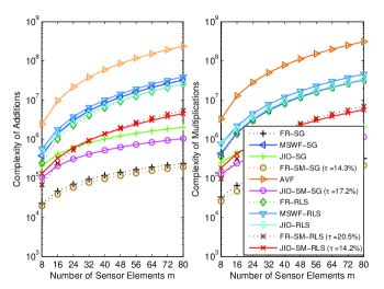
Figure 2: Complexity in terms of arithmetic operations versus the number of sensor elements $m$.

V-B Stability Analysis

In order to establish conditions for the stability of the proposed JIO-SM-SG algorithm, we define $\boldsymbol{e}_{T}(i)=\boldsymbol{T}_{r}(i)-\boldsymbol{T}_{r,\textrm{opt}}$ and $\boldsymbol{e}_{\bar{w}}(i)=\bar{\boldsymbol{w}}(i)-\bar{\boldsymbol{w}}_{\textrm{opt}}$ with $\boldsymbol{T}_{r,\textrm{opt}}$ and $\bar{\boldsymbol{w}}_{\textrm{opt}}$ being the optimal solutions of the transformation matrix and the reduced-rank filter, respectively. The expression of $\boldsymbol{T}_{r,\textrm{opt}}$ can be obtained by taking the gradient of (10) with respect to $\boldsymbol{T}_{r}$, i.e., $\boldsymbol{T}_{r,\textrm{opt}}=\frac{\gamma\boldsymbol{R}\boldsymbol{a}(\theta_{0})}{\boldsymbol{a}^{H}(\theta_{0})\boldsymbol{R}\boldsymbol{a}(\theta_{0})}\frac{\bar{\boldsymbol{w}}_{\textrm{opt}}^{H}}{\|\bar{\boldsymbol{w}}_{\textrm{opt}}\|^{2}}$, where $\bar{\boldsymbol{w}}_{\textrm{opt}}$ has been given in (6). By substituting (11) and (12) into $\boldsymbol{e}_{T}(i)$ and $\boldsymbol{e}_{\bar{w}}(i)$, respectively, and rearranging the terms, we have

$$\begin{split}\boldsymbol{e}_{T}(i+1)=\boldsymbol{T}_{1}(i)\boldsymbol{e}_{T}(i)-\mu_{T}(i)\boldsymbol{T}_{2}(i)+\mu_{T}(i)\boldsymbol{T}_{3}(i),\end{split}$$ (24)

$$\boldsymbol{e}_{\bar{w}}(i+1)=\bar{\boldsymbol{W}}_{1}(i)\boldsymbol{e}_{\bar{w}}(i)-\mu_{\bar{w}}(i)\bar{\boldsymbol{W}}_{2}(i),$$ (25)

where
$\boldsymbol{T}_{1}(i)=\boldsymbol{I}-\mu_{T}(i)[\boldsymbol{I}-\frac{\boldsymbol{a}(\theta_{0})\boldsymbol{a}^{H}(\theta_{0})}{{\boldsymbol{a}}^{H}(\theta_{0}){\boldsymbol{a}}(\theta_{0})}]\boldsymbol{x}(i)\boldsymbol{x}^{H}(i)$;
$\boldsymbol{T}_{2}(i)=[\boldsymbol{I}-\frac{\boldsymbol{a}(\theta_{0})\boldsymbol{a}^{H}(\theta_{0})}{{\boldsymbol{a}}^{H}(\theta_{0}){\boldsymbol{a}}(\theta_{0})}]\boldsymbol{x}(i)\boldsymbol{x}^{H}(i)\bar{\boldsymbol{w}}^{H}(i)\boldsymbol{e}_{\bar{w}}(i)\boldsymbol{T}_{r}(i)$;
$\boldsymbol{T}_{3}(i)=[\boldsymbol{I}-\frac{\boldsymbol{a}(\theta_{0})\boldsymbol{a}^{H}(\theta_{0})}{{\boldsymbol{a}}^{H}(\theta_{0}){\boldsymbol{a}}(\theta_{0})}]\boldsymbol{x}(i)\boldsymbol{x}^{H}(i)[(1-\bar{\boldsymbol{w}}^{H}(i)\bar{\boldsymbol{w}}_{\textrm{opt}})\boldsymbol{T}_{r}(i)-\boldsymbol{T}_{r,\textrm{opt}}]$;
$\bar{\boldsymbol{W}}_{1}(i)=\boldsymbol{I}-\mu_{\bar{w}}(i)[\boldsymbol{I}-\frac{\bar{\boldsymbol{a}}(\theta_{0})\bar{\boldsymbol{a}}^{H}(\theta_{0})}{\bar{\boldsymbol{a}}^{H}(\theta_{0})\bar{\boldsymbol{a}}(\theta_{0})}]\bar{\boldsymbol{x}}(i)\bar{\boldsymbol{x}}^{H}(i)$;
$\bar{\boldsymbol{W}}_{2}(i)=[\boldsymbol{I}-\frac{\bar{\boldsymbol{a}}(\theta_{0})\bar{\boldsymbol{a}}^{H}(\theta_{0})}{\bar{\boldsymbol{a}}^{H}(\theta_{0})\bar{\boldsymbol{a}}(\theta_{0})}]\bar{\boldsymbol{x}}(i)\bar{\boldsymbol{x}}^{H}(i)\bar{\boldsymbol{w}}_{\textrm{opt}}$.

Since we are dealing with a joint optimization procedure, both the transformation matrix and the reduced-rank filter have to be considered jointly. Besides, the time-varying bound should be investigated. By substituting (13) and (14) into (24) and (25), respectively, and taking expectations, we get

$$\begin{bmatrix}\mathbb{E}[\boldsymbol{e}_{T}(i+1)]\\ \mathbb{E}[\boldsymbol{e}_{\bar{w}}(i+1)]\\ \end{bmatrix}=\begin{bmatrix}\boldsymbol{U}_{1}&\boldsymbol{0}\\ \boldsymbol{0}&\bar{\boldsymbol{U}}_{2}\\ \end{bmatrix}\begin{bmatrix}\mathbb{E}[\boldsymbol{e}_{T}(i)]\\ \mathbb{E}[\boldsymbol{e}_{\bar{w}}(i)]\\ \end{bmatrix}+\begin{bmatrix}\boldsymbol{V}_{1}\\ \bar{\boldsymbol{V}}_{2}\\ \end{bmatrix},$$ (26)

where
$\boldsymbol{U}_{1}=\boldsymbol{I}-\frac{\big{(}1-\frac{\delta(i)}{|y(i)|}\big{)}[\boldsymbol{I}-\frac{\boldsymbol{a}(\theta_{0})\boldsymbol{a}^{H}(\theta_{0})}{{\boldsymbol{a}}^{H}(\theta_{0}){\boldsymbol{a}}(\theta_{0})}]\boldsymbol{x}(i)\boldsymbol{x}^{H}(i)}{\|\bar{\boldsymbol{w}}(i)\|^{2}\boldsymbol{x}^{H}(i)[\boldsymbol{I}-\frac{\boldsymbol{a}(\theta_{0})\boldsymbol{a}^{H}(\theta_{0})}{{\boldsymbol{a}}^{H}(\theta_{0}){\boldsymbol{a}}(\theta_{0})}]\boldsymbol{x}(i)}$;
$\bar{\boldsymbol{U}}_{2}=\boldsymbol{I}-\frac{\big{(}1-\frac{\delta(i)}{|y(i)|}\big{)}[\boldsymbol{I}-\frac{\bar{\boldsymbol{a}}(\theta_{0})\bar{\boldsymbol{a}}^{H}(\theta_{0})}{\bar{\boldsymbol{a}}^{H}(\theta_{0})\bar{\boldsymbol{a}}(\theta_{0})}]\bar{\boldsymbol{x}}(i)\bar{\boldsymbol{x}}^{H}(i)}{\bar{\boldsymbol{x}}^{H}(i)[\boldsymbol{I}-\frac{\bar{\boldsymbol{a}}(\theta_{0})\bar{\boldsymbol{a}}^{H}(\theta_{0})}{\bar{\boldsymbol{a}}^{H}(\theta_{0})\bar{\boldsymbol{a}}(\theta_{0})}]\bar{\boldsymbol{x}}(i)}$;
${\boldsymbol{V}}_{1}=\frac{\big{(}1-\frac{\delta(i)}{|y(i)|}\big{)}[-\boldsymbol{T}_{2}(i)+\boldsymbol{T}_{3}(i)]}{\|\bar{\boldsymbol{w}}(i)\|^{2}\boldsymbol{x}^{H}(i)[\boldsymbol{I}-\frac{\boldsymbol{a}(\theta_{0})\boldsymbol{a}^{H}(\theta_{0})}{{\boldsymbol{a}}^{H}(\theta_{0}){\boldsymbol{a}}(\theta_{0})}]\boldsymbol{x}(i)}$;
$\bar{\boldsymbol{V}}_{2}=-\frac{\big{(}1-\frac{\delta(i)}{|y(i)|}\big{)}\bar{\boldsymbol{W}}_{2}(i)}{\bar{\boldsymbol{x}}^{H}(i)[\boldsymbol{I}-\frac{\bar{\boldsymbol{a}}(\theta_{0})\bar{\boldsymbol{a}}^{H}(\theta_{0})}{\bar{\boldsymbol{a}}^{H}(\theta_{0})\bar{\boldsymbol{a}}(\theta_{0})}]\bar{\boldsymbol{x}}(i)}$.

From (26), it implies that the stability of the proposed JIO-SM-SG algorithm depends on the spectral radius of $\boldsymbol{U}=\textrm{diag}[\boldsymbol{U}_{1},\bar{\boldsymbol{U}}_{2}]$. The step size values should satisfy the condition that the eigenvalues of $\boldsymbol{U}^{H}\boldsymbol{U}$ are less than one for convergence. The variable step size values calculated by (13) and (14) follow this condition with the bounded constraint. Unlike the stability analysis of existing adaptive algorithms, the terms in the proposed algorithm are more involved and depend on each other as evidenced by the equations in $\boldsymbol{U}$, $\boldsymbol{V}_{1}$ and $\bar{\boldsymbol{V}}_{2}$.

V-C Prediction of The Trend of MSE

In this part, we derive expressions to predict the trend of the MSE for the proposed JIO-SM-SG algorithm. The following analysis begins with the conventional MSE analysis of [6] and then involves the novel parameters $\boldsymbol{T}_{r}(i)$ and $\bar{\boldsymbol{w}}(i)$ due to the joint optimization property. The data-selective updates of the SMF technique is also considered in the analysis by introducing a new coefficient $P_{e}(i)$ in the update equations.

Let us define the the estimation error at time instant $i$ to be

$$e(i)=d_{0}(i)-y(i)=e_{0}(i)-\boldsymbol{e}_{w}^{H}(i)\boldsymbol{x}(i),$$ (27)

where $d_{0}(i)$ denotes the transmitted data of the desired user, $\boldsymbol{e}_{w}(i)=\boldsymbol{w}(i)-\boldsymbol{w}_{\textrm{opt}}$ with $\boldsymbol{w}_{\textrm{opt}}$ being the optimal weight solution, and $e_{0}(i)=d_{0}(i)-\boldsymbol{w}_{\textrm{opt}}^{H}\boldsymbol{x}(i)$. The filter $\boldsymbol{w}(i)=\boldsymbol{T}_{r}(i)\bar{\boldsymbol{w}}(i)$ with $m$ parameters is the $r$-rank approximation of a full-rank filter obtained with an inverse transformation [21] processed by $\boldsymbol{T}_{r}(i)$.

The MSE following the time instant $i$ is given by

$$\begin{split}J_{\textrm{mse}}(i)&=\mathbb{E}[|e(i)|^{2}]\\ &=J_{\textrm{min}}+\mathbb{E}[\boldsymbol{e}_{w}^{H}(i)\boldsymbol{R}\boldsymbol{e}_{w}(i)]\\ &=J_{\textrm{min}}+\sigma_{x}^{2}\textrm{tr}\{\textrm{cov}[\boldsymbol{e}_{w}(i)]\}\end{split}$$ (28)

where $J_{\textrm{min}}$ is the minimum MSE (MMSE) produced by the optimal LCMV solution and $\sigma_{x}^{2}\textrm{tr}\{\textrm{cov}[\boldsymbol{e}_{w}(i)]\}$ denotes the excess MSE (EMSE) with $\sigma_{x}^{2}=B_{0}^{2}b_{0}^{2}+B_{1}^{2}b_{1}^{2}+\ldots+B_{q-1}^{2}b_{q-1}^{2}$ being the summed variance of the transmitted data and $B_{k}$ ($k=0,\ldots,q-1$) being the amplitude. Assuming $d_{k}$ is independent and identically distributed (i.i.d.), the MMSE can be expressed by

$$\begin{split}J_{\textrm{min}}&=\mathbb{E}[|e_{0}(i)|^{2}]\\ &=\mathbb{E}[|d_{0}(i)|^{2}]-\boldsymbol{w}_{\textrm{opt}}^{H}\boldsymbol{a}(\theta_{0})-\boldsymbol{a}^{H}(\theta_{0})\boldsymbol{w}_{\textrm{opt}}+\boldsymbol{w}_{\textrm{opt}}^{H}\boldsymbol{R}\boldsymbol{w}_{\textrm{opt}}.\end{split}$$ (29)

Considering the inverse transformation, the weight error vector becomes,

$$\begin{split}\boldsymbol{e}_{w}(i)&=\boldsymbol{T}_{r}(i)\bar{\boldsymbol{w}}(i)-\boldsymbol{T}_{r,\textrm{opt}}\bar{\boldsymbol{w}}_{\textrm{opt}}\\ &=\boldsymbol{e}_{T}(i)\boldsymbol{e}_{\bar{w}}(i)+\boldsymbol{T}_{r,\textrm{opt}}\boldsymbol{e}_{\bar{w}}(i)+\boldsymbol{e}_{T}(i)\bar{\boldsymbol{w}}_{\textrm{opt}}.\end{split}$$ (30)

To provide further analysis, we use (11) and (12) and consider the data-selective updates of the SMF technique given by

$$\boldsymbol{T}_{r}(i+1)=\boldsymbol{T}_{r}(i)-P_{e}(i)\mu_{T}(i)y^{\ast}(i)\big{[}\boldsymbol{I}-\frac{\boldsymbol{a}(\theta_{0})\boldsymbol{a}^{H}(\theta_{0})}{{\boldsymbol{a}}^{H}(\theta_{0}){\boldsymbol{a}}(\theta_{0})}\big{]}\boldsymbol{x}(i)\bar{\boldsymbol{w}}^{H}(i),$$ (31)

$$\bar{\boldsymbol{w}}(i+1)=\bar{\boldsymbol{w}}(i)-P_{e}(i)\mu_{\bar{w}}(i)y^{\ast}(i)\big{[}\boldsymbol{I}-\frac{\bar{\boldsymbol{a}}(\theta_{0})\bar{\boldsymbol{a}}^{H}(\theta_{0})}{\bar{\boldsymbol{a}}^{H}(\theta_{0})\bar{\boldsymbol{a}}(\theta_{0})}\big{]}\bar{\boldsymbol{x}}(i),$$ (32)

where $\mu_{T}(i)$ and $\mu_{\bar{w}}(i)$ are the variable step size values following the time-varying bound, and $P_{e}(i)$ is a coefficient modeling the probability of updating the filter parameters with respect to a given time instant $i$, namely, $P_{e}(i)=P[|y(i)|^{2}>\delta^{2}(i)]$. Note that $P_{e}(i)$ is same for (31) and (32) since $\boldsymbol{T}_{r}(i)$ and $\bar{\boldsymbol{w}}(i)$ depend on each other and update jointly.

Substituting (31) and (32) into (30) and making some rearrangements, we have

$$\begin{split}\boldsymbol{e}_{w}(i+1)=&\boldsymbol{e}_{w}(i)-P_{e}(i)\mu_{T}(i)y^{\ast}(i)\boldsymbol{G}_{r}(i)\bar{\boldsymbol{w}}(i)\\ &-P_{e}(i)\mu_{\bar{w}}(i)y^{\ast}(i)\boldsymbol{T}_{r}(i)\bar{\boldsymbol{g}}(i)\\ &+P_{e}^{2}(i)\mu_{T}(i)\mu_{\bar{w}}(i)[y^{\ast}(i)]^{2}\boldsymbol{G}_{r}(i)\boldsymbol{g}(i),\end{split}$$ (33)

where $\boldsymbol{G}_{r}(i)=\big{[}\boldsymbol{I}-\boldsymbol{a}(\theta_{0})\boldsymbol{a}^{H}(\theta_{0})\big{]}\boldsymbol{x}(i)\bar{\boldsymbol{w}}^{H}(i)$, and $\bar{\boldsymbol{g}}(i)=\big{[}\boldsymbol{I}-\frac{\bar{\boldsymbol{a}}(\theta_{0})\bar{\boldsymbol{a}}^{H}(\theta_{0})}{\bar{\boldsymbol{a}}^{H}(\theta_{0})\bar{\boldsymbol{a}}(\theta_{0})}\big{]}\bar{\boldsymbol{x}}(i)$. By using (13) and (14) and applying $y(i)=\bar{\boldsymbol{w}}^{H}(i)\bar{\boldsymbol{x}}(i)$ to (30), we get

$$\begin{split}\boldsymbol{e}_{w}(i+1)=[\boldsymbol{I}-\boldsymbol{V}(i)]\boldsymbol{e}_{w}(i)-\boldsymbol{V}(i)\boldsymbol{w}_{\textrm{opt}}+\tau(i)\boldsymbol{G}_{r}(i)\bar{\boldsymbol{g}}(i),\end{split}$$ (34)

where
$\boldsymbol{V}(i)=P_{e}(i)[1-\frac{\delta(i)}{|y(i)|}][\frac{\boldsymbol{G}_{r}(i)\bar{\boldsymbol{w}}(i)\boldsymbol{x}^{H}(i)}{\bar{\boldsymbol{w}}^{H}(i)\boldsymbol{G}_{r}^{H}(i)\boldsymbol{x}(i)}+\frac{\boldsymbol{T}_{r}(i)\bar{\boldsymbol{g}}(i)\boldsymbol{x}^{H}(i)}{\bar{\boldsymbol{x}}^{H}(i)\bar{\boldsymbol{g}}(i)}]$;
$\tau(i)=P_{e}^{2}(i)[y^{\ast}(i)]^{2}\frac{[1-\frac{\delta(i)}{|y(i)|}]^{2}}{\bar{\boldsymbol{w}}^{H}(i)\boldsymbol{G}_{r}^{H}(i)\boldsymbol{x}(i)\bar{\boldsymbol{x}}^{H}(i)\bar{\boldsymbol{g}}(i)}$.

The last step is to give a $P_{e}(i)$ in order to provide good estimates. In [33], a fixed probability that approximates the update rate of the parameters is introduced. Here, we use a modified version and involve the time-varying bound in our time-varying probability, which is

$$P_{e}(i)=2Q\big{(}\frac{\delta(i)}{\sigma_{n}}\big{)}+P_{\textrm{min}},$$ (35)

where $Q(\cdot)$ is the complementary Gaussian cumulative distribution given by $Q(x)=\int_{x}^{\infty}\frac{1}{\sqrt{2\pi}}e^{-t^{2}/2}dt$, and $P_{\textrm{min}}$ is prior information about the minimum update rate for the proposed algorithm to reach a relatively high performance. Both $P_{e}(i)$ and $P_{\textrm{min}}$ are different with respect to different $N$ and reflect the data-selective updating behavior as $N$ increases. The term $P_{\textrm{min}}$ is a certain value if the number of snapshots is fixed.

The weight error vector can be calculated via its updating equation (34). The MSE value of the proposed JIO-SM-SG algorithm at a given time instant $i$ can be obtained by substituting (34) into (28), which is

$$\begin{split}&J_{\textrm{mse}}(i+1)=J_{\textrm{min}}\\ &+\sigma_{x}^{2}\textrm{tr}\Big{\{}\textrm{cov}\big{\{}[\boldsymbol{I}-\boldsymbol{V}(i)]\boldsymbol{e}_{w}(i)-\boldsymbol{V}(i)\boldsymbol{w}_{\textrm{opt}}+\tau(i)\boldsymbol{G}_{r}(i)\bar{\boldsymbol{g}}(i)\big{\}}\Big{\}}\end{split}$$ (36)

This analysis provides a means to predict the trend of the MSE performance of the proposed algorithm. In the next section, we use the simulation result to verify the validity of the analysis.

V-D Analysis of The Optimization Problem

In this part, we provide an analysis based on the optimization problem in (9) and show a condition that allows the designer to avoid local minima associated with the proposed optimization problem. The analysis also considers the bounded constraint and the constraint on the steering vector of the SOI to illustrate the properties of the problem. Our analysis starts from the transformation of the array output $y(i)$ in a more convenient form and then substitutes its expression into the constrained optimization problem to render the analysis. For simplicity, we drop the time instant $i$ in the quantities.

From (1), the array output can be written as:

$$\begin{split}y&=\bar{\boldsymbol{w}}^{H}\boldsymbol{T}_{r}^{H}\big{\{}\sum_{k=0}^{q-1}\boldsymbol{a}(\theta_{k})s_{k}+\boldsymbol{n}\big{\}}\\ &=\bar{\boldsymbol{w}}^{H}\sum_{k=0}^{q-1}\sum_{j=1}^{r}\boldsymbol{S}_{k}\big{[}\boldsymbol{t}_{j}^{H}\boldsymbol{a}(\theta_{k})\boldsymbol{\nu}_{j}\big{]}+\bar{\boldsymbol{w}}^{H}\boldsymbol{I}\sum_{j=1}^{r}\boldsymbol{t}_{j}^{H}\boldsymbol{n}\boldsymbol{\nu}_{j},\end{split}$$ (37)

where $\boldsymbol{S}_{k}\in\mathbb{C}^{r\times r}$ is a diagonal matrix with all its main diagonal entries equal to the transmitted data of the $k$th user, i.e., $s_{k}$, $\boldsymbol{t}_{j}\in\mathbb{C}^{m\times 1}$ is the $j$th column vector of the transformation matrix $\boldsymbol{T}_{r}$, and $\boldsymbol{\nu}_{j}\in\mathbb{C}^{r\times 1}$ is a vector containing a $1$ in the $j$th position and zeros elsewhere. In order to proceed, we define

$$\begin{split}\mathbb{S}_{k}=\begin{bmatrix}\boldsymbol{0}&\boldsymbol{0}\\ \boldsymbol{S}_{k}&\boldsymbol{0}\end{bmatrix};\mathbb{S}_{n}=\begin{bmatrix}\boldsymbol{0}&\boldsymbol{0}\\ \boldsymbol{S}_{n}&\boldsymbol{0}\end{bmatrix};\boldsymbol{f}_{k}=\begin{bmatrix}\bar{\boldsymbol{w}}^{\ast}\\ \boldsymbol{T}_{r}^{T}\boldsymbol{a}_{k}^{\ast}\end{bmatrix};\boldsymbol{f}_{n}=\begin{bmatrix}\bar{\boldsymbol{w}}^{\ast}\\ \boldsymbol{T}_{r}^{T}\boldsymbol{n}^{\ast}\end{bmatrix},\end{split}$$ (38)

where $\mathbb{S}_{k}\in\mathbb{C}^{2r\times 2r}$, $\mathbb{S}_{n}\in\mathbb{C}^{2r\times 2r}$ are the signal matrix containing the transmitted signal of the $k$th user and the noise matrix containing $\boldsymbol{n}$, respectively, and $\boldsymbol{f}_{k}\in\mathbb{C}^{2r\times 1}$ and $\boldsymbol{f}_{n}\in\mathbb{C}^{2r\times 1}$ are the parameter vector containing the steering vector of the $k$th user and the noise vector related to $\boldsymbol{n}$, respectively.

According to (38), the array output can be expressed by

$$y=\sum_{k=0}^{q-1}\boldsymbol{f}_{k}^{H}\mathbb{S}_{k}\boldsymbol{f}_{k}+\boldsymbol{f}_{n}^{H}\mathbb{S}_{n}\boldsymbol{f}_{n},$$ (39)

where we notice that, if $k=0$, it has $\boldsymbol{f}_{0}^{H}\mathbb{S}_{0}\boldsymbol{f}_{0}=\bar{\boldsymbol{w}}^{H}\boldsymbol{T}_{r}^{H}\boldsymbol{a}(\theta_{0})s_{0}=\gamma s_{0}$, which is based on the constraint on the steering vector of the SOI in (9). The expression in (39) involves this constraint in the array output and thus will simplify the derivation when substituting into the optimization problem. This is also the reason why we use (39) instead of $y=\bar{\boldsymbol{w}}^{H}\boldsymbol{T}_{r}^{H}\boldsymbol{x}$ for the analysis.

Before taking the analysis further, we use two assumptions. First, the signals are assumed to be transmitted independently. Second, we consider a noise free case [34] or a sufficiently high signal-to-noise ratio (SNR) condition. Under these assumptions, using the Lagrange multiplier method, the optimization problem in (9) can be written as

$$\begin{split}J(\boldsymbol{T}_{r},\bar{\boldsymbol{w}})&=\mathbb{E}[|y|^{2}]+2\lambda\mathfrak{R}[|y|^{2}-\delta^{2}]\\ &=\mathbb{E}[\sum_{k=0}^{q-1}\boldsymbol{f}_{k}^{H}\mathbb{S}_{k}\boldsymbol{f}_{k}\boldsymbol{f}_{k}^{H}\mathbb{S}_{k}^{H}\boldsymbol{f}_{k}]\\ &~{}~{}~{}+2\lambda\mathfrak{R}[\sum_{k=0}^{q-1}\sum_{l=0}^{q-1}\boldsymbol{f}_{k}^{H}\mathbb{S}_{k}\boldsymbol{f}_{k}\boldsymbol{f}_{l}^{H}\mathbb{S}_{l}^{H}\boldsymbol{f}_{l}-\delta^{2}],\end{split}$$ (40)

where the constraint on the steering vector of the SOI is not included since it has been enclosed in (39).

In order to evaluate the property of (40), we can verify if the Hessian matrix $\boldsymbol{H}_{0}$ [35] with respect to $\boldsymbol{f}_{0}$ of the desired user is positive semi-definite for all nonzero vector $\boldsymbol{u}$ with $\boldsymbol{u}^{H}\boldsymbol{H}_{0}\boldsymbol{u}\geq 0$. Computing the Hessian of the above optimization problem for the desired user we obtain

$$\begin{split}\boldsymbol{H}_{0}&=\frac{\partial}{\partial\boldsymbol{f}_{0}^{H}}\frac{\partial J}{\partial\boldsymbol{f}_{0}}\\ &=\mathbb{E}\big{[}\boldsymbol{H}_{01}+\boldsymbol{H}_{02}\big{]}+2\lambda\mathfrak{R}\big{[}\boldsymbol{H}_{01}+\boldsymbol{H}_{02}+\boldsymbol{H}_{03}\big{]},\end{split}$$ (41)

where
$\boldsymbol{H}_{01}=\mathbb{S}_{0}\boldsymbol{f}_{0}\boldsymbol{f}_{0}^{H}\mathbb{S}_{0}^{H}+\mathbb{S}_{0}^{H}\boldsymbol{f}_{0}\boldsymbol{f}_{0}^{H}\mathbb{S}_{0}$;
$\boldsymbol{H}_{02}=\boldsymbol{f}_{0}^{H}\mathbb{S}_{0}^{H}\boldsymbol{f}_{0}\mathbb{S}_{0}+\boldsymbol{f}_{0}^{H}\mathbb{S}_{0}\boldsymbol{f}_{0}\mathbb{S}_{0}^{H}$;
$\boldsymbol{H}_{03}=\sum_{k=1}^{q-1}\boldsymbol{f}_{k}^{H}\mathbb{S}_{k}^{H}\boldsymbol{f}_{k}\mathbb{S}_{k}+\sum_{l=1}^{q-1}\boldsymbol{f}_{l}^{H}\mathbb{S}_{l}\boldsymbol{f}_{l}\mathbb{S}_{l}^{H}$. According to the constraint, $\boldsymbol{H}_{02}=2\mathfrak{R}[\gamma^{\ast}s_{0}^{\ast}\mathbb{S}_{0}]$. From (41), $\boldsymbol{H}_{01}$ yields a positive semi-definite matrix, while $\boldsymbol{H}_{03}$ is an undetermined term. Thus, for avoiding the local minima associated with the optimization problem, a sufficient condition is to guarantee

$$\boldsymbol{H}_{0}^{\prime}=\mathbb{E}[\boldsymbol{H}_{02}]+2\lambda\mathfrak{R}[\boldsymbol{H}_{02}+\boldsymbol{H}_{05}],$$ (42)

to be positive semi-definite, i.e., $\boldsymbol{u}^{H}\boldsymbol{H}_{0}^{\prime}\boldsymbol{u}\geq 0$. This task can be achieved by selecting an appropriate Lagrange multiplier $\lambda$. For the Hessian matrix with respect to the other users, $\boldsymbol{H}_{k}$ ($k=1,\ldots,q-1$), we could use the same way to avoid the local minima of the optimization problem.

VI Simulations

In this section, we evaluate the performance of the proposed JIO-SM-SG and JIO-SM-RLS adaptive algorithms for designing LCMV beamformers and compare them with existing algorithms. Specifically, we compare the proposed algorithms with the full-rank (FR) SG and RLS algorithms [6] with/without the SMF technique, and the reduced-rank algorithms based on the MSWF [12] and the AVF [17] techniques. In all simulations, we assume that there is one desired user in the system and the related DOA is known beforehand by the receiver. All the results are averaged by $1000$ runs. The input signal-to-interference ratio (SIR) is SIR=$-20$ dB. We consider the binary phase shift keying (BPSK) modulation scheme and set $\gamma=1$ for the studied algorithms. Simulations are performed with a ULA containing $m=64$ sensor elements with half-wavelength interelement spacing. We consider $m$ large in order to show their advantages of the proposed algorithms in terms of performance and computational complexity when the number of elements in the beamformer is large.

In Fig. 3, we assess the impact of the rank $r$ on the output signal-to-interference-plus-noise ratio (SINR) performance of the proposed and existing algorithms. There are $q=25$ users in the system whose DoAs are generated with uniform random variables between $0$ and $180$ degrees. The input SNR is SNR=$10$ dB. In order to show the convergence behavior, we set the total number of snapshots to $N=300$. The value of the rank $r$ is chosen between $1$ and $10$ because reduced-rank adaptive algorithms usually show the best performance for these values [13, 32]. A reduced-rank algorithm with a lower rank (e.g., $r=3$) often converges quickly whereas a reduced-rank technique with a larger rank (e.g., $r=8$) reaches a higher SINR level at steady state. We have chosen the parameters $\alpha=22$, $\beta=0.99$, $\mu_{T}(1)=\mu_{\bar{w}}(1)=0.05$ for the proposed JIO-SM-SG algorithm, and $\alpha=26$, $\beta=0.992$, $\rho=1.3\times 10^{-3}$, $\varrho=1.0\times 10^{-4}$ for the proposed JIO-SM-RLS algorithm in order to optimize the performance of the algorithms. By changing these parameters, the performance will be degraded, the update rate will decrease if the threshold $\delta$ is large, whereas the update rate will increase if the threshold $\delta$ is small. Note that $\lambda_{1}(i)$ should be in accordance with the setting of the forgetting factor and thus $0.1\leq\lambda_{1}(i)\leq 0.998$ is used for implementation. Fig. 3 suggests that the most adequate rank for the proposed algorithms to obtain the best performance in this example is $r=5$, which is equal to or lower in comparison to the existing reduced-rank algorithms. Besides, we also checked that this rank value is rather insensitive to the number of users or interferers in the system, to the number of sensor elements, and work efficiently for the scenarios considered in the next examples. Since the best $r$ is usually much smaller than the number of elements $m$, it leads to a significant computational reduction. In general, we may expect some variations for the optimal rank $r$ which should be in the range $3<r<10$. In the following simulations, we use $r=5$ for the proposed algorithms.

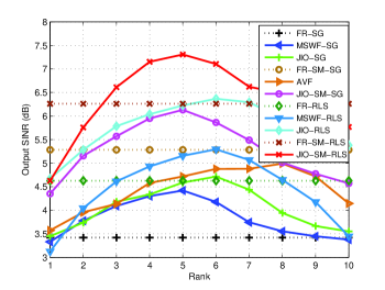
Figure 3: Output SINR versus the number of rank $r$.

In Fig. 4, we evaluate the SINR performance of the proposed and existing algorithms versus the number of snapshots. It includes two experiments, which compare the SG-based and the RLS-based algorithms. The AVF algorithm is included in both experiments to make a clear comparison. The scenario and the coefficients for the proposed algorithms are the same as in Fig. 3. The number of snapshots is $N=1000$. In Fig. 4 (a), the JIO-based algorithms show a better convergence rate than other full-rank and reduced-rank algorithms. The proposed JIO-SM-SG algorithm has a good performance and only requires $17.2\%$ updates ($172$ updates for $1000$ snapshots), reducing the computational cost. Fig. 4 (b) exhibits a similar result for the RLS-based algorithms. The JIO-SM-RLS converges quickly to the steady-state, which is close to the minimum variance distortionless response (MVDR) solution [3]. The update rate is $\tau=14.2\%$, which is much lower than its reduced-rank counterparts that require $100\%$ updates.

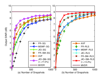
Figure 4: Output SINR versus the number of snapshots for (a) SG-based algorithms; (b) RLS-based algorithms.

Fig. 5 shows the SINR performance of the proposed algorithms with the fixed and time-varying bounds. The scenario is the same as that in Fig. 3. From Fig. 5 (a), we find that the curve with the fixed bound $\delta=1.0$ has comparable SINR values to the proposed one as the number of snapshots increases. The reason is that we use the BPSK modulation scheme and thus the absolute value of the ideal array output should equal $1$, which follows the constraint and achieves high SINR values. However, it requires more updates ($\tau=44.8\%$) and has to afford a much higher computational load. The curves with higher ($\delta=1.4$) or lower ($\delta=0.8$) bounds exhibit the worse convergence performance. The proposed JIO-SM-SG algorithm with the time-varying bound performs the data-selective updates to obtain a good tradeoff between the complexity and the performance. The same result can be found in Fig. 5 (b) for the proposed JIO-SM-RLS algorithm, which uses even less updates to obtain an enhanced performance.

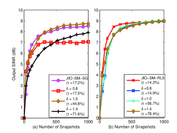
Figure 5: Output SINR versus the number of snapshots for (a) SG-based algorithms; (b) RLS-based algorithms.

In the next experiment, we consider a non-stationary scenario, namely, when the number of users changes in the system, and check the tracking performance of the proposed algorithms. The system starts with $q=20$ users including one desired user. The coefficients are $r=5$, $\alpha=18$, $\beta=0.99$, $\mu_{T}(1)=\mu_{\bar{w}}(1)=0.05$ for the proposed JIO-SM-SG algorithm and $r=5$, $\alpha=19$, $\beta=0.995$, $\rho=1.3\times 10^{-3}$, $\varrho=1\times 10^{-4}$ for the proposed JIO-SM-RLS algorithm. From Fig. 6, the proposed algorithms achieve a superior convergence performance to the other compared algorithms. The environment experiences a sudden change at $i=1500$. We have $10$ interferers entering the system. This change degrades the SINR performance for all the algorithms. The proposed algorithms track this change and converge rapidly to the steady-state since the data-selective updates reduce the number of parameter estimation and thus keep a faster convergence rate. Besides, the time-varying bound provides information for them to follow the changes of the scenario. It is clear that the proposed algorithms still keep low update rates ($\tau=15.3\%$ for the JIO-SM-SG and $\tau=16.0\%$ for the JIO-SM-RLS even under non-stationary conditions.

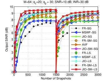
Figure 6: Output SINR versus the number of snapshots in dynamic scenario with additional users enter and/or leave the system.

In the last experiment, the simulated and analytical results in Subsection V-C for the proposed JIO-SM-SG algorithm are compared. The simulated curves are obtained via simulations in Fig. 7 and the predicted ones are from (36). In this scenario, there are $q=20$ users in the system and INR$=25$ dB. We compare the results with two different SNR values, i.e., SNR$=5$ dB and SNR$=10$ dB. The coefficients are $\alpha=9.7$, $\beta=0.99$, $\mu_{T}(1)=\mu_{\bar{w}}(1)=0.05$, and $r=5$. To get the predicted MSE, we set $P_{\textrm{min}}=17.0\%$ (for SNR=$5$ dB) and $P_{\textrm{min}}=16.3\%$ (for SNR=$10$ dB), which are in accordance with the update rates of the simulated MSE and provide a fair comparison. From Fig. 7, the predicted curves agree with the simulated ones, especially when $i\geq 200$, verifying the validity of our analysis. Note that there is a small gap between the simulated and predicted curves at the beginning. The reason is that the number of snapshots is insufficient for the proposed JIO-SM-SG algorithm to provide accurate estimates if $i\leq m$ (or before the algorithm converges to the steady-state). The update rates for the simulated curves are quite low and thus decrease the computational cost for the proposed algorithm.

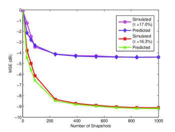
Figure 7: MSE performance versus the number of snapshots for the proposed JIO-SM-SG algorithm.

VII Concluding Remarks

We have introduced a new reduced-rank framework that incorporates the SMF technique into the reduced-rank JIO scheme for beamforming. According to this framework, we have considered reduced-rank LCMV designs with a bounded constraint on the amplitude of the array output, and developed SG-based and RLS-based adaptive algorithms for beamforming. The proposed algorithms have employed the received data to construct a space of feasible solutions for the updates. They have a superior convergence and an enhanced tracking performance over their existing counterparts due to the iterative exchange of information between the transformation matrix and the reduced-rank weight vector. In addition, the proposed algorithms can save computational costs due to the data-selective updates. A time-varying bound was employed to adjust the step size values for the SG-based algorithm and the forgetting factor values for the RLS-based algorithm, making the proposed algorithms more robust to dynamic scenarios. The results have shown the advantages of the proposed algorithms and verified the analytical formulas derived.

Derivation of JIO-SG Algorithm

The recursions for the JIO-SG algorithms are derived from (10). Fixing $\bar{\boldsymbol{w}}$ and computing the gradient terms of (10) with respect to ${\boldsymbol{T}}_{r}$ and using a gradient descent rule [Diniz], we have

$${\boldsymbol{T}}_{r}[i+1]={\boldsymbol{T}}_{r}[i]-\mu_{T}(y^{*}[i]{\boldsymbol{x}}[i]\bar{\boldsymbol{w}}^{H}[i]+2\eta{\boldsymbol{a}}(\theta_{0})\bar{\boldsymbol{w}}^{H}[i]).$$ (43)

Substituting the above into the constraint $\bar{\boldsymbol{w}}^{H}[i]{\boldsymbol{T}}_{r}^{H}[i]{\boldsymbol{a}}(\theta_{0})=\gamma$, we obtain the value of the Lagrange multiplier

$$\eta=1/2({\boldsymbol{a}}^{H}(\theta_{0}){\boldsymbol{a}}(\theta_{0}))^{-1}{\boldsymbol{a}}^{H}(\theta_{0}){\boldsymbol{x}}[i]y^{*}[i]$$ (44)

Substituting $\eta$ into (43), we obtain (11). The recursion for $\bar{\boldsymbol{w}}$ is obtained by an analogous gradient descent rule

$$\bar{\boldsymbol{w}}[i+1]=\bar{\boldsymbol{w}}[i]-\mu_{w}(y^{*}[i]{\boldsymbol{T}}_{r}^{H}[i]{\boldsymbol{x}}[i]+2\eta{\boldsymbol{T}}_{r}^{H}[i]{\boldsymbol{a}}(\theta_{0})).$$ (45)

Using the constraint again with the above recursion, we can obtain the value for the Lagrange multiplier for use in the update of $\bar{\boldsymbol{w}}$ and which results in (13).

Derivation of Variable Step Size Values

In this appendix, we derive the expressions in (13) and (14). We drop the time instant $i$ for simplicity. According to the optimization problem, substituting (11) into the bounded constraint in (9), we have

$$\Big{|}\bar{\boldsymbol{w}}^{H}\Big{\{}\boldsymbol{T}_{r}^{H}-\mu_{T}^{\ast}y\big{[}\bar{\boldsymbol{w}}{\boldsymbol{x}}^{H}-{\bar{\boldsymbol{w}}\boldsymbol{x}^{H}\boldsymbol{a}(\theta_{0})\boldsymbol{a}^{H}(\theta_{0})}\big{]}\Big{\}}\boldsymbol{x}\Big{|}=\delta$$ (46)

The above equation can be expressed in an alternative form, which is

$$\Big{|}y-\mu_{T}^{\ast}y\bar{\boldsymbol{w}}^{H}\bar{\boldsymbol{w}}\boldsymbol{x}^{H}\big{[}\boldsymbol{I}-\boldsymbol{a}(\theta_{0})\boldsymbol{a}^{H}(\theta_{0})\big{]}\boldsymbol{x}\Big{|}=\delta$$ (47)

Making an arrangement to (47), we obtain the variable step size expression for the transformation matrix in (13).

Also, substituting (12) into the bounded constraint, we obtain

$$\Big{|}\bar{\boldsymbol{w}}^{H}\bar{\boldsymbol{x}}-\mu_{\bar{w}}^{\ast}y\bar{\boldsymbol{x}}^{H}[\boldsymbol{I}-\frac{\bar{\boldsymbol{a}}(\theta_{0})\bar{\boldsymbol{a}}^{H}(\theta_{0})}{\bar{\boldsymbol{a}}^{H}(\theta_{0})\bar{\boldsymbol{a}}(\theta_{0})}]\bar{\boldsymbol{x}}\Big{|}=\delta,$$ (48)

where the expression of $\mu_{\bar{w}}$ in (14) can be obtained by performing mathematical transformations to (48).

Derivation of (16)

In this appendix, we derive the expression of the transformation matrix in (16). Given $\bar{\boldsymbol{w}}(i)\neq\boldsymbol{0}$, taking the gradient of (15) with respect to $\boldsymbol{T}_{r}(i)$, we have

$$\begin{split}\nabla J_{\boldsymbol{T}_{r}(i)}=&\sum_{l=1}^{i-1}\lambda_{1}^{i-l}(i)\boldsymbol{x}(l)\boldsymbol{x}^{H}(l)\boldsymbol{T}_{r}(i)\bar{\boldsymbol{w}}(i)\bar{\boldsymbol{w}}^{H}(i)\\ &+\lambda_{1}(i)\boldsymbol{x}(i)\boldsymbol{x}^{H}(i)\boldsymbol{T}_{r}(i)\bar{\boldsymbol{w}}(i)\bar{\boldsymbol{w}}^{H}(i)+\lambda_{2}\boldsymbol{a}(\theta_{0})\bar{\boldsymbol{w}}^{H}(i).\end{split}$$ (49)

Making $\nabla J_{\boldsymbol{T}_{r}(i)}=\boldsymbol{0}$ and right-multiplying the both sides by $\bar{\boldsymbol{w}}(i)$, and rearranging the expression, it becomes

$$\boldsymbol{T}_{r}(i)\bar{\boldsymbol{w}}(i)=-\lambda_{2}\big{[}\sum_{l=1}^{i-1}\lambda^{i-l}_{1}(i)\boldsymbol{x}(l)\boldsymbol{x}^{H}(l)+\lambda_{1}(i)\boldsymbol{x}(i)\boldsymbol{x}^{H}(i)\big{]}^{-1}\boldsymbol{a}(\theta_{0}).$$ (50)

Considering the assumption $\lambda_{1}(i)\rightarrow 1$ and using the matrix inversion lemma, we have

$$\begin{split}\boldsymbol{T}_{r}(i)\bar{\boldsymbol{w}}(i)&=-\lambda_{2}\big{[}\boldsymbol{R}(i-1)+\lambda_{1}(i)\boldsymbol{x}(i)\boldsymbol{x}^{H}(i)\big{]}^{-1}\boldsymbol{a}(\theta_{0})\\ &=-\lambda_{2}\boldsymbol{P}(i)\boldsymbol{a}(\theta_{0}),\end{split}$$ (51)

where $\boldsymbol{P}(i)$ has been given in (18).

Let $\boldsymbol{v}(i)=\boldsymbol{P}(i)\boldsymbol{a}(\theta_{0})$, the solution of $\boldsymbol{T}_{r}(i)$ can be regarded to find the solution to the linear equation

$$\boldsymbol{T}_{r}(i)\bar{\boldsymbol{w}}(i)=\boldsymbol{v}(i),$$ (52)

where there exists multiple $\boldsymbol{T}_{r}(i)$ satisfying this equation if only $\bar{\boldsymbol{w}}\neq\boldsymbol{0}$. We derive the minimum Frobenius-norm solution for stability. We write $\boldsymbol{T}_{r}(i)$ and $\boldsymbol{v}(i)$ in the form of

$$\boldsymbol{T}_{r}(i)=\begin{bmatrix}\bar{\boldsymbol{t}}_{1}(i)\\ \bar{\boldsymbol{t}}_{2}(i)\\ \vdots\\ \bar{\boldsymbol{t}}_{m}(i)\\ \end{bmatrix};~{}~{}{\boldsymbol{v}}(i)=\begin{bmatrix}v_{1}(i)\\ v_{2}(i)\\ \vdots\\ v_{m}(i)\\ \end{bmatrix},$$ (53)

where $\bar{\boldsymbol{t}}_{j}\in\mathbb{C}^{r\times 1}$ with $j=1,\ldots,m$ denotes the row vector of the transformation matrix. Thus, the search of the minimum Frobenius-norm solution is simplified to the following $m$ subproblems:

$$\textrm{minimize}~{}\|\bar{\boldsymbol{t}}_{j}(i)\|^{2},~{}~{}\textrm{subject~{}to}~{}~{}\bar{\boldsymbol{t}}_{j}(i)\bar{\boldsymbol{w}}(i)=v_{j}(i).$$ (54)

Solving the constrained optimization problem in (54), we have

$$\bar{\boldsymbol{t}}_{j}(i)=v_{j}(i)\frac{\bar{\boldsymbol{w}}^{H}(i)}{\|\bar{\boldsymbol{w}}(i)\|^{2}}.$$ (55)

Substituting (55) into (52) and considering the definition of $\boldsymbol{v}(i)$, the minimum Frobenius-norm solution is given by

$$\boldsymbol{T}_{r}(i)=-\lambda_{2}\boldsymbol{P}(i)\boldsymbol{a}(\theta_{0})\frac{\bar{\boldsymbol{w}}^{H}(i)}{\|\bar{\boldsymbol{w}}(i)\|^{2}},$$ (56)

where $\lambda_{2}$ can be obtained by incorporating (51) into the constraint with respect to $\boldsymbol{a}(\theta_{0})$, which is

$$\lambda_{2}=-\frac{\gamma}{\boldsymbol{a}^{H}(\theta_{0})\boldsymbol{P}(i)\boldsymbol{a}(\theta_{0})}.$$ (57)

References

- [1]
- [2] D. H. Johnson and D. E. Dudgeon, Array Signal Processing: Concepts and Techniques. Englewood Cliffs, NJ: Prentice-Hall, 1993.
- [3] H. L. Van Trees, Detection, Estimation, and Modulation, Part IV, Optimum Array Processing,” John Wiley & Sons, 2002.
- [4] O. L. Frost, “An algorithm for linearly constrained adaptive array processing,” IEEE Proc., AP-30, pp. 27-34, 1972.
- [5] R. C. de Lamare and R. Sampaio-Neto, “Low-Complexity Variable Step-Size Mechanisms for Stochastic Gradient Algorithms in Minimum Variance CDMA Receivers”, IEEE Trans. Signal Processing, vol. 54, pp. 2302 - 2317, June 2006.
- [6] S. Haykin, Adaptive Filter Theory, 4rd ed., Englewood Cliffs, NJ: Prentice-Hall, 1996.
- [7] A. Massa, P. Rocca, R. Haupt, ”Interference Suppression in Uniform Linear Arrays through a Dynamic Thinning Strategy,” IEEE Transactions on Antennas and Propagation, to appear.
- [8] M. D’Urso, T. Isernia, E. F. Meliado, ”An Effective Hybrid Approach for the Optimal Synthesis of Monopulse Antennas,” IEEE Transactions on Antennas and Propagation, vol.55, no.4, pp.1059-1066, April 2007.
- [9] R. L. Haupt, ”Optimized Weighting of Uniform Subarrays of Unequal Sizes,” IEEE Transactions on Antennas and Propagation, vol.55, no.4, pp.1207-1210, April 2007.
- [10] R. L. Haupt, D. W. Aten, ”Low Sidelobe Arrays via Dipole Rotation,” IEEE Transactions on Antennas and Propagation, vol.57, no.5, pp.1575-1579, May 2009.
- [11] R. L. Haupt, J. Flemish, D. Aten, ”Adaptive Nulling Using Photoconductive Attenuators,” IEEE Transactions on Antennas and Propagation, vol.59, no.3, pp.869-876, March 2011.
- [12] M. L. Honig and W. Xiao, “Performance of reduced-rank linear interference suppression,” IEEE Trans. Information Theory, vol. 47, pp. 1928-1946, July 2001.
- [13] J. S. Goldstein, I. S. Reed, and L. L. Scharf, “A multistage representation of the Wiener filter based on orthogonal projections,” IEEE Trans. Information Theory, vol. 44, pp. 2943-2959, Nov. 1998.
- [14] D.J. Rabideau, “Closed-loop multistage adaptive beamforming”, Proc. Conference Record of the Thirty-Third Asilomar Conference on Signals, Oct. 24-27 1999.
- [15] M. L. Honig and J. S. Goldstein, “Adaptive reduced-rank interference suppression based on the multistage Wiener filter,” IEEE Trans. Communications, vol. 50, pp. 986-994, June 2002.
- [16] R. C. de Lamare, M. Haardt, and R. Sampaio-Neto, “Blind adaptive constrained reduced-rank parameter estimation based on constant modulus design for CDMA interference suppression,” IEEE Trans. Signal Proc., vol. 56, pp. 2470-2482, Jun. 2008.
- [17] D. A. Pados and G. N. Karystinos, “An iterative algorithm for the computation of the MVDR filter,” IEEE Trans. Signal Processing, vol. 49, pp. 290-300, Feb. 2001.
- [18] B. L. Mathews, L. Mili, and A. I. Zaghloul, “Auxiliary vector selection algorithms for adaptive beamforming,” IEEE Conf. Antenna and Propagation Society International Symposium, vol. 3A, pp. 271-274, 2005.
- [19] R. C. de Lamare and R. Sampaio-Neto, “Reduced-rank adaptive filtering based on joint iterative optimization of adaptive filters,” IEEE Signal Processing Letters, vol. 14, pp. 980-983, Dec. 2007.
- [20] R. C. de Lamare, ”Adaptive Reduced-Rank LCMV Beamforming Algorithms Based on Joint Iterative Optimisation of Filters,” Electronics Letters, vol. 44, no. 9, April 24, pp. 565 - 566.
- [21] R. C. de Lamare, L. Wang, and R. Fa, “Adaptive reduced-rank LCMV beamforming algorithms based on joint iterative optimization of filters: design and analysis,” Signal Processing, vol. 90, pp. 640-652, Feb. 2010.
- [22] R. C. de Lamare and R. Sampaio-Neto, ”Reduced-Rank Space-Time Adaptive Interference Suppression With Joint Iterative Least Squares Algorithms for Spread-Spectrum Systems,” IEEE Trans. on Vehicular Technology, vol.59, no.3, March 2010, pp.1217-1228.
- [23] R. Fa and R. C. de Lamare, ”Reduced-Rank STAP Algorithms using Joint Iterative Optimization of Filters,” IEEE Trans. on Aerospace and Electronic Systems, vol.47, no.3, pp.1668-1684, July 2011.
- [24] R. C. de Lamare and R. Sampaio-Neto, “Adaptive Reduced-Rank Processing Based on Joint and Iterative Interpolation, Decimation, and Filtering,” IEEE Trans. on Signal Processing, vol. 57, no. 7, July 2009, pp. 2503 - 2514.
- [25] R. Fa, R. C. de Lamare and L. Wang, “Reduced-rank STAP schemes for airborne radar based on switched joint interpolation, decimation and filtering algorithm”, IEEE Trans. Sig. Proc., 2010, vol. 58, no. 8, pp.4182-4194.
- [26] R.C. de Lamare, R. Sampaio-Neto and M. Haardt, ”Blind Adaptive Constrained Constant-Modulus Reduced-Rank Interference Suppression Algorithms Based on Interpolation and Switched Decimation,” IEEE Trans. on Signal Processing, vol.59, no.2, pp.681-695, Feb. 2011.
- [27] S. Gollamudi, S. Nagaraj, S. Kapoor, and Y. Huang, “Set-membership filtering and a set-membership normalized LMS algorithm with an adaptive step size,” IEEE Signal Processing Letters, vol. 5, pp. 111-114, May 1998.
- [28] S. Nagaraj, S. Gollamudi, S. Kapoor, and Y. Huang, “BEACON: an adaptive set-membership filtering technique with spars updates,” IEEE Trans. Signal Processing, vol. 47, pp. 2928-2940, Nov. 1999.
- [29] L. Guo and Y. F. Huang, “Frequency-domain set-membership filtering and its applications,” IEEE Trans. Signal Processing, vol. 55, pp. 1326-1338, Apr. 2007.
- [30] L. Guo and Y. F. Huang, “Set-membership adaptive filtering with parameter-dependent error bound tuning,” IEEE Proc. Int. Conf. Acoust. Speech and Signal Processing, 2005.
- [31] R. C. de Lamare and P. S. R. Diniz, “Set-membership adaptive algorithms based on time-varying error bounds for CDMA interference suppression,” IEEE Trans. Vehicular Technology, vol. 58, pp. 644-654, Feb. 2009.
- [32] L. Wang, R. C. de Lamare, and M. Yukawa, “Adaptive reduced-rank constrained constant modulus algorithms based on joint iterative optimization of filters for beamforming,” IEEE Trans. Signal Processing, vol. 58, pp. 2983-2997, June 2010.
- [33] M. V. S. Lima and P. S. R. Diniz, “Steady-state analysis of the set-membership affine projection algorithm,” Proc. IEEE ICASSP, Dallas, Texas, pp. 3802-3805, Mar. 2010.
- [34] C. J. Xu, G. Z. Feng, and K. S. Kwak, “A modified constrained constant modulus approach to blind adaptive multiuser detection,” IEEE Trans. Communications, vol. 49, pp. 1642-1648, Sep. 2001.
- [35] D. Luenberger and Y. Ye, Linear and Nonlinear Programming, 3rd. Ed. Springer Science&Business Media, 2008.
- [36]
- [37] U. Niesen, D. Shah, and G. W. Wornell, “Adaptive Alternating Minimization Algorithms”, IEEE Trans. Inform. Theory, vol. 55, no. 3, pp. 1423-1429, Mar. 2009.
- [38]