Electromagnetic quasinormal modes of rotating black strings and the AdS/CFT correspondence

Abstract:

We investigate the quasinormal spectrum of electromagnetic perturbations of rotating black strings. Among the solutions of Einstein equations in the presence of a negative cosmological constant there are asymptotically anti-de Sitter (AdS) black holes whose horizons have the topology of a cylinder. The stationary version of these AdS black holes represents rotating black strings. The conformal field theory (CFT) dual of a black string lives in a Minkowski space with a compact dimension. On the basis of the AdS/CFT duality, we interpret a CFT plasma moving with respect to the preferred rest frame introduced by the topology as the holographic dual to a rotating black string. We explore the consequences of this correspondence by investigating the electromagnetic perturbations of a black string for different rotation parameter values. As usual the electromagnetic quasinormal modes (QNM) correspond to the poles of retarded Green’s functions of $R$-symmetry currents in the boundary field theory. The hydrodynamic regime of the QNM dispersion relations are analytically studied. Finally, we investigate numerically the effect of rotation on all the family of black-string electromagnetic quasinormal modes. We interpret these results from the CFT perspective and notice the emergence of effects like Doppler shift of the frequencies and dilation of the thermalization times.

1 Introduction

During the last decade the AdS/CFT correspondence [1, 2, 3, 4] at nonzero temperature and density has become part of the basic toolkit for those who seek to investigate in- and out-of-equilibrium properties of systems described by quantum field theories at strong coupling regime. There is now a variety of bottom-up and top-down AdS/QCD models being used to study many problems in strong interactions like the computation of deep inelastic structure functions, the hadronic spectra and the energy loss by heavy quarks in a plasma (for reviews on the subject see refs. [5, 6, 7, 8, 9, 10, 11]). More recently, the AdS/CFT duality has been applied to study condensed-matter systems. High-temperature superconductivity, quantum and classical Hall effects, and the (non-)Fermi liquid behavior of some materials are among the physical phenomena that were investigated by means of holographic methods. An excellent account of these developments can be found in refs. [12, 13, 14].

Investigations within the AdS/CFT framework have also uncover new aspects of blackhole physics as the existence of a scalar-hair instability of Reissner-Nordström-$\mbox{AdS}_{4}$ black holes in the regime of low Hawking’s temperature [15, 16]. Such an effect opens the possibility of a charged black hole having a superfluid phase, and the consequent existence of holographic superfluids [17]. Another important outcome was the association of hydrodynamics to black hole physics not only in asymptotically AdS spacetimes, but even for more general backgrounds. In fact, the first suggestions of applying fluid mechanics to the study of event-horizon dynamics come from the old ‘membrane paradigm’ approach [18, 19, 20, 21, 22]. However, this idea has only began to take form with the computation of transport coefficients via AdS/CFT, and received a great impulse with the advent of the so-called fluid/gravity correspondence: a one-to-one mapping between solutions of the relativistic Navier-Stokes equation and the long-wavelength regime of perturbations of black holes [23, 24, 25, 26]. Among some of the interesting results arising from fluid/gravity duality are the universality of the ratio of the shear viscosity to the entropy density for all large-$N$ gauge theories with a dual Einstein gravity [27]; the equivalent for static fluids between area minimization of the fluid and area maximization of the black hole horizon; and the connection between surface tension of the fluid and surface gravity of the corresponding black hole [28].

The AdS/CFT duality gave rise to a series of results involving traditional black holes, as well as it allowed new interpretations of blackhole spacetimes with unusual topology, specially in higher than four spacetime dimensions. One of the first studied blackhole solutions with a non-spherical topology in anti-de Sitter spacetime involves a plane-symmetric black hole solution [29, 30, 31]. In addition to the change of the asymptotic behavior of the blackhole spacetime, the presence or absence of a cosmological constant determines the different topologies that a black hole may have. In asymptotically flat four-dimensional spacetimes, a series of theorems assures that the event horizon of black holes are necessarily spherical. This is a characteristic of all black holes forming the Kerr-Newman family. However, the situation changes as soon as we add a negative cosmological constant term to the Einstein field equations. The corresponding solutions do not represent globally hyperbolic spacetimes and the theorems regarding the blackhole topology cannot be applied. It also allows solutions of the Einstein equations which have all the properties of a blackhole solution, but with event horizons presenting non-trivial topologies. Particularly, there are asymptotically AdS spacetimes for which the spherical horizons of the Schwarzschild-AdS black holes are exchanged by a plane or a hyperboloid. In the plane-symmetric case, in addition to the usual planar $\mathbb{R}^{2}$ topology, it is possible to identify points in the plane surface in order to generate horizons with multiply connected topologies. The resulting surface can be orientable as the cylinder and the flat torus or non-orientable like the Möbius band and Klein bottle [32]. In the cylindrical case, the so-called black string (or cylindrical black hole) can also be put to rotate through a ‘forbidden’ coordinate transformation in the sense of Stachel [33], which mixes time with angular coordinates and generates new geometries representing rotating blackhole-like background, i.e., a rotating black string [34]. The rotating black string is the object of study in the present work. In the case of the toroidal topology, the black hole can also be put to rotate, but the analysis is similar and we do not deal with it here.

The quasinormal modes (QNM) of asymptotically anti-de Sitter black holes have been intensively studied in the last decade (For recent reviews on QNM, see e.g. [35, 36]). The main interest in such a study is the AdS/CFT interpretation in which the electromagnetic and gravitational quasinormal frequencies of anti-de Sitter black holes are associated respectively to the poles of retarded correlation functions of R-symmetry currents and stress-energy tensor in the holographically dual conformal field theory. According to the dictionary of the duality, a black hole in the AdS bulk is dual to a CFT thermal state in the AdS spacetime boundary, and, in particular, as we shall show in the present work, a rotating black string is the holographic dual to a CFT plasma moving with respect to the preferred rest frame introduced by the topology.

We investigate the quasinormal spectrum of electromagnetic perturbations of rotating black strings. Even though the quasinormal oscillations of rotating black holes with spherical horizon, such as the Kerr-AdS black holes, have been studied in detail in the literature, the case of rotating black strings has not being analyzed yet. We then take such a task and find the dispersion relations for a few values of the rotation parameter by using the Horowitz-Hubeny numerical method [37]. Approximate analytical expressions for the dispersion relations in the hydrodynamic limit are also found. From the CFT perspective we notice the emergence of effects like the Doppler shift of frequencies, wavelength contraction and dilation of the thermalization times.

The layout of the present article is as follows. In the next section, for completeness, it is reviewed a known plane-symmetric static blackhole solution of Einstein equations in $(3+1)$ dimensions and a brief summary of how the rotating black string can be found from the static solution. In the sequence the metric of the rotating black string is rewritten in a form that is completely covariant regarding to the spacetime boundary. In section 3 the electromagnetic perturbation equations are decoupled in transverse and longitudinal sectors. Analytical results are obtained and discussed in section 4. Section 5 is dedicated to presenting and analyzing the numerical results and, finally, in section 6 we conclude by commenting on the main results.

In relation to the units, we are going to use natural units throughout this paper, i.e., the speed of light $c$, Boltzmann constant $k_{\scriptscriptstyle{B}}$, and Planck constant $\hbar$ are all set to unity, $c=k_{\scriptscriptstyle{B}}=\hbar=1$. Capital Latin indices ($M,\,N,\,...$) run over all the spacetime dimensions, while Greek indices ($\mu,\,\nu,\,...$) run over the coordinates of the AdS boundary.

2 The background spacetime

2.1 The static black string

The background spacetime we start with is a plane-symmetric static blackhole solution of Einstein equations in $(3+1)$ dimensions. Such a spacetime presents a physical singularity, and a negative cosmological constant $\Lambda$, which renders the background geometry asymptotically anti-de Sitter. In Schwarzschild-like coordinates, the spacetime metric takes the form [29, 34, 30, 31]

$$ds^{2} = -\alpha^{2}r^{2}f(r)\,d\bar{t}^{\,2}+\dfrac{dr^{2}}{\alpha^{2}r^{2}\,f(r)}+\alpha^{2}r^{2}\left(dx^{2}+dy^{2}\right),$$ (1)

$$f(r) = 1-\frac{b}{\alpha^{3}r^{3}},$$ (2)

where $\alpha=1/R=\sqrt{-\Lambda/3}$ and $b$ is a constant related to the ADM mass of the source. As usual, usual, coordinates $\bar{t}$ and $r$ are assumed to have the ranges $-\infty<{\bar{t}}<+\infty$, $0\leq r<+\infty$. The two-dimensional surfaces ($S$) of constant $\bar{t}$ and constant $r$ may have different topologies. In addition to the usual topology of a plane ($\mathbb{R}\times\mathbb{R}$), if one or two of the coordinates $x$ and $y$ are periodic the surface $S$ has the topology of a cylinder ($\mathbb{R}\times\mathbb{S}^{1}$) or of a torus ($\mathbb{S}^{1}\times\mathbb{S}^{1}$), respectively (see, e.g., [38] for a review and more references on this subject). Other multiply connected choices are the Möbius band and the Klein bottle, but these are not interesting for the present study because the corresponding spaces are non-orientable.

In this work we are interested in studying the QNM of rotating AdS black holes and the interesting cases are the cylindrical black holes ($\mathbb{R}\times\mathbb{S}^{1}$) and the toroidal black holes ($\mathbb{S}^{1}\times\mathbb{S}^{1}$). We consider such cases because, as it was shown in ref. [34], these black solutions allow the addition of angular momentum by coordinate transformations (see, also [33]), generating new spacetimes which represent rotating black strings and rotating black tori, respectively. On the other hand, if the dimensions are not compactified the spacetime (1) can not be put to rotate thereby.

To clarify notation, it is interesting to redefine coordinates as follows: $\alpha x\rightarrow\bar{\varphi}$ and $y\rightarrow z$, with $0\leq\bar{\varphi}<2\pi$ and $-\infty<z<+\infty$, for the cylindrical case; or $\alpha x\rightarrow\bar{\varphi}$ and $\alpha y\rightarrow\bar{\theta}$, with $0\leq\bar{\varphi}<2\pi$ and $0\leq\bar{\theta}<2\pi$, for the toroidal case. Since the ranges of the angular (compactified) coordinates are arbitrary, we have chosen these particular ranges for convenience. As mentioned above, parameter $b$ is related to the mass per unit length $M$ of the static black string, $b=4M$, with $M$ standing for the linear mass density, in the cylindrical case, and with $M$ representing the total gravitational mass of the black hole, in the toroidal case.

The spacetime (1) presents an event horizon at $r={r_{h}}$, with

$$r_{h}=\dfrac{b^{1/3}}{\alpha}=\dfrac{\left(4M\right)^{1/3}}{\alpha}$$ (3)

and an essential singularity at $r=0$. The Hawking temperature of the black hole is given by

$${\mathcal{T}}=\frac{3r_{h}\alpha^{2}}{4\pi}=\frac{3r_{h}}{4\pi R^{2}},$$ (4)

where we have put $\hbar=1$.

2.2 The rotating black string

For the sake of clarity in presentation, and to avoid confusion, we restrict the description to the cylindrical case (black string). The analysis of the toroidal black hole is easily obtained by further compactifying along the $y$ direction in metric (1). The consequences of such an additional compactification shall not be analyzed in the present work.

According to Stachel [33], a forbidden coordinate transformation of a static black string (cylindrical black hole) generates a rotating black string. In this way, Lemos [34] obtained a rotating black string from the metric given in equation (1). We then consider such a solution here by performing the following linear transformation that mixes the timelike and angular coordinates:

$$\left\{\begin{aligned} &\bar{t}=\gamma\left(t-{a}\,\varphi\right),\\ &\bar{\varphi}=\gamma\left(\varphi-a\alpha^{2}t\right).\end{aligned}\right.$$ (5)

After changing from $(x,\,y)$ to $(\bar{\varphi},\,z)$ in (1) and applying the local transformation (5) to the resulting metric one obtains

$$ds^{2}=-{\alpha^{2}r^{2}}\gamma^{2}f(r)\left(dt-ad\varphi\right)^{2}+{\alpha^{2}r^{2}}\gamma^{2}\left(\dfrac{d\varphi}{\alpha}-{a\,\alpha}dt\right)^{2}+{\alpha^{2}r^{2}}dz^{2}+\frac{dr^{2}}{\alpha^{2}r^{2}f(r)}\;,$$ (6)

where $\gamma$ and $a$ are chosen to satisfy $\gamma^{2}\left(1-{\alpha^{2}}a^{2}\right)=1$ in order to have the usual anti-de Sitter form of metric at spatial infinity. Then one has

$${\gamma}=\dfrac{1}{\sqrt{1-a^{2}\alpha^{2}}}.$$ (7)

The ranges of the new coordinates are $-\infty<{t}<+\infty$, $0\leq r<+\infty$, $0\leq{\varphi}<2\pi$ and $-\infty<z<+\infty$, so that metric (6) represents a rotating cylindrical black hole spacetime.

The stationary metric (6), of course, satisfies Einstein equations with negative cosmological constant $\Lambda=-3\alpha^{2}$. Due to the non-trivial spacetime topology, (5) is a global forbidden coordinate transformation and thus metrics (1) and (6) represent two distinct spacetimes.

As shown initially by Lemos [34] and generalized by including electric charge in ref. [39], for cylindrical topology ($\mathbb{R}\times\mathbb{S}^{1}$), and for $a^{2}\alpha^{2}\leq 1$, the metric (6) describes the spacetime of a rotating black string. The conserved mass $M$ and the conserved angular momentum $J$ per unit length of the black string are given in terms of the parameters $a$ and $b$ through the relations

$$M=b\gamma^{2}\left(\frac{2+a^{2}\alpha^{2}}{8}\right),\quad\qquad J=\frac{3ab\gamma^{2}}{8},$$ (8)

or, inverting for $a$ and $b$,

$$b=-2\left(M-\sqrt{9M^{2}-8\alpha^{2}J^{2}}\right),\qquad a=\frac{3M-\sqrt{9M^{2}-8\alpha^{2}J^{2}}}{2\alpha^{2}J}.$$ (9)

In terms of $M$ and $J$, the condition of existence of an event horizon $a^{2}\alpha^{2}\leq 1$ becomes $J^{2}\alpha^{2}\leq M^{2}$, and the horizon function $f(r)=1-b/\alpha^{3}r^{3}$ reads

$$f(r)=1-\left(3\sqrt{1-\dfrac{8}{9}\dfrac{J^{2}\alpha^{2}}{M^{2}}}\;-1\right)\left(\dfrac{2M}{\alpha^{3}r^{3}}\right),$$ (10)

and in terms of $M$ and $a$ it is

$$f(r)=1-\left(\dfrac{3\sqrt{4+a^{2}\alpha^{2}\left(a^{2}\alpha^{2}-4\right)}}{2+a^{2}\alpha^{2}}-1\right)\left(\dfrac{2M}{\alpha^{3}r^{3}}\right).$$ (11)

For $0\leq J\leq M/\alpha$, metric (6) has a horizon at $r=r_{h}$, where $r_{h}$ is given by

$$r_{h}^{3}=\frac{b}{\alpha^{3}}=\;2\frac{\sqrt{9M^{2}-8J^{2}\alpha^{2}}-M}{\alpha^{3}},$$ (12)

or

$$r_{h}^{3}=\frac{b}{\alpha^{3}}=\left(\dfrac{3\sqrt{4+a^{2}\alpha^{2}\left(a^{2}\alpha^{2}-4\right)}}{2+a^{2}\alpha^{2}}-1\right)\left(\dfrac{2M}{\alpha^{3}}\right).$$ (13)

As in the case of the static spacetime (2.1), the region $r=0$ is an essential spacelike singularity, and the region $r\rightarrow\infty$ is the AdS boundary. The case $J^{2}=M^{2}/\alpha^{2}$ ($a^{2}\alpha^{2}=1$) is the extremal limit of the rotating black string, in which the horizon radius vanishes and the singularity $r=0$ becomes lightlike. This particular case is of no interest for the present study.

The Hawking temperature of the rotating black string is given by [34]

$$T=\frac{3\alpha}{4\pi}\left[2\left({\,\sqrt{9M^{2}-8J^{2}\alpha^{2}}-M}\right)\right]^{1/3}\left[\frac{3\sqrt{9M^{2}-8J^{2}\alpha^{2}}-3M}{\sqrt{9M^{2}-8J^{2}\alpha^{2}}+3M}\right]^{1/2},$$ (14)

or, in terms of the horizon radius and the rotation parameter $a$,

$$T=\frac{3r_{h}\alpha^{2}}{4\pi}\sqrt{1-a^{2}\alpha^{2}}=\mathcal{T}\sqrt{1-a^{2}\alpha^{2}},$$ (15)

where $\mathcal{T}$ is the temperature of a static black string with the same horizon radius as its rotating counterpart. For $J=0$ ($a=0$), Hawking temperature (15) reduces to the temperature of the static black string, given by relation (4), as expected. Moreover, for extremal rotating black strings ($J=M/\alpha$) the Hawking temperature vanishes, similarly to the case of extremal black holes in asymptotically Minkowski spacetimes.

Introducing the coordinates $x^{\mu}=(x^{0},x^{1},x^{2})=(t,\,\varphi/\alpha,\,z)$ and the velocity

$$U^{\mu}=(U^{0},U^{1},U^{2})=\gamma\left(1,\,a\,\alpha,\,0\right)$$ (16)

on the boundary of the spacetime, i.e., at $r\longrightarrow\infty$, the metric of the rotating black string (6) can be cast into the form [40, 23]

$$ds^{2}=\frac{dr^{2}}{\alpha^{2}r^{2}f(r)}+\alpha^{2}r^{2}\left[-f(r)U_{\mu}U_{\nu}+h_{\mu\nu}\right]dx^{\mu}dx^{\nu},$$ (17)

where $h_{\mu\nu}$ is the projector onto the orthogonal direction to $U_{\mu}$,

$$h_{\mu\nu}=\eta_{\mu\nu}+U_{\mu}U_{\nu},$$ (18)

and $\eta_{\mu\nu}$ is the Minkowski metric at the boundary, $\eta_{\mu\nu}=(-1,1,1)$.

The components of the inverse metric tensor $g^{MN}$ are given by

$$g^{MN}=\left\{\displaystyle{\begin{array}[]{ll}g^{rr}=\alpha^{2}r^{2}f(r),\quad g^{r\mu}=g^{\mu r}=0,\\ g^{\mu\nu}=\dfrac{1}{\alpha^{2}r^{2}}\left[-\dfrac{U^{\mu}U^{\nu}}{f(r)}+h^{\mu\nu}\right],\end{array}}\right.$$ (19)

where the indices of the quantities defined at the boundary, such as $U_{\mu}$ and $h_{\mu\nu}$, are raised (lowered) by the Minkowski metric $\eta^{\mu\nu}=\eta_{\mu\nu}={\rm diag}(-1,1,1)$. With this notation, we can find the perturbation equations of a given field for an arbitrary velocity $U_{\mu}$. The case of an electromagnetic field as a perturbation in the above spacetime is analyzed and the electromagnetic quasinormal modes are studied in the following. Even though the geometry of the rotating black string is locally similar to that of the static black string, the QNM of the rotating black string are expected to be different from that of the static case because the QNM depend upon the global structure of the spacetimes, which are certainly different from each other.

3 Fundamental equations for the perturbations

Considering the electromagnetic field as a perturbation on the rotating black string (17), the resulting equations of motion for the gauge field $A_{\scriptscriptstyle{M}}$ are the usual Maxwell equations

$$\partial_{\scriptscriptstyle{M}}[\sqrt{-g}g^{\scriptscriptstyle{MN}}g^{\scriptscriptstyle{LP}}F_{\scriptscriptstyle{NP}}]=0,$$ (20)

where $g_{\scriptscriptstyle{MN}}$ stands for the metric components given by (17), with capital Latin indices running over all the spacetime dimensions ($M,\,N=0,\,1,\,2,\,3$), and the Maxwell tensor $F_{\scriptscriptstyle{MN}}$ being related to gauge field $A_{\scriptscriptstyle{M}}$ by

$$F_{\scriptscriptstyle{MN}}=\partial_{\scriptscriptstyle{M}}A_{\scriptscriptstyle{N}}-\partial_{\scriptscriptstyle{N}}A_{\scriptscriptstyle{M}}.$$ (21)

We consider fluctuations of the gauge field in terms of Fourier transforms as follows

$$A_{\scriptscriptstyle{M}}(x^{\mu},r)=\int\frac{dx^{3}}{(2\pi)^{3}}e^{ik_{\mu}x^{\mu}}\widetilde{A}_{\scriptscriptstyle{M}}(k^{\mu},r),$$ (22)

where Greek indices run over the coordinates of the AdS boundary, and $k^{\mu}$ is the wave vector defined at the spacetime boundary ($\mu,\,\nu=0,\,1,\,2$). The components of the wave vector along compact spatial directions are in fact quantized numbers. In the present case, such components are multiples of $\alpha$, the inverse of the anti-de Sitter radius.

The equations of motion (20) for the gauge field (22) together with appropriate boundary conditions give the QNM dispersion relations for this field. Since the Maxwell equations are invariant under the gauge transformation $A_{\scriptscriptstyle{M}}\rightarrow A_{\scriptscriptstyle{M}}+\partial_{\scriptscriptstyle{M}}\lambda$, we may choose $\lambda$ in such a way to vanish one of the components of $A_{\scriptscriptstyle{M}}$. We adopt the so-called radial gauge, in which $A_{r}=0$. With such a choice, we find that the gauge field perturbations satisfy the following equations

$$k_{\scriptscriptstyle{\parallel}}\partial_{r}A_{\scriptscriptstyle{\parallel}}-f\,\partial_{r}(k_{\scriptscriptstyle{\perp}}^{\nu}A_{\nu})=0,$$ (23)

$$\begin{split}&\alpha^{4}r^{2}f\,\left[\partial_{r}\left(r^{2}f\,\partial_{r}A^{\mu}_{\scriptscriptstyle{\perp}}\right)-U^{\mu}\partial_{r}\left(r^{2}\partial_{r}A_{\scriptscriptstyle{\parallel}}\right)\right]+k{\scriptscriptstyle{\parallel}}\left(k_{\scriptscriptstyle{\parallel}}A_{\scriptscriptstyle{\perp}}^{\mu}-A{\scriptscriptstyle{\parallel}}k_{\scriptscriptstyle{\perp}}^{\mu}\right)\\ &+U^{\mu}k^{\sigma}_{\scriptscriptstyle{\perp}}\left(k_{\sigma}A_{\scriptscriptstyle{\parallel}}-A_{\sigma}k_{\scriptscriptstyle{\parallel}}\right)-f\,k^{\sigma}_{\scriptscriptstyle{\perp}}\left(k_{\sigma}A^{\mu}_{\scriptscriptstyle{\perp}}-A_{\sigma}k^{\mu}_{\scriptscriptstyle{\perp}}\right)=0,\end{split}$$ (24)

where, to simplify notation, the tilde was dropped, $\widetilde{A}_{\mu}\rightarrow A_{\mu}$. The index $\perp$ (‖) indicates the projection of a given object onto the perpendicular (parallel) direction to the velocity $U^{\mu}$. In particular, the longitudinal (parallel) component of the perturbation gauge field is defined by $A_{\scriptscriptstyle{\parallel}}=U^{\nu}A_{\nu}$, while the transverse vector is $A_{\scriptscriptstyle{\perp}}^{\mu}=h^{\mu\nu}A_{\nu}$.

The system of equations (23)–(24) can be decoupled into two independent (parallel and transverse with respect to the velocity $U^{\mu}$) channels. We first project equation (24) onto the parallel direction to the velocity $U^{\mu}$, obtaining

$$\alpha^{4}r^{2}f\,\partial_{r}\left(r^{2}\partial_{r}A_{\scriptscriptstyle{\parallel}}\right)-k^{2}_{\scriptscriptstyle{\perp}}A_{\scriptscriptstyle{\parallel}}+(k^{\sigma}_{\scriptscriptstyle{\perp}}A_{\sigma})k_{\scriptscriptstyle{\parallel}}=0,$$ (25)

where we have used the identities $k_{\scriptscriptstyle{\perp}}^{2}=k_{\scriptscriptstyle{\perp}}^{\sigma}k_{{\scriptscriptstyle{\perp}}\sigma}=k_{\scriptscriptstyle{\perp}}^{\sigma}k_{\sigma}$. On the other hand, projecting equation (24) onto the transverse spatial direction to the velocity $U^{\mu}$ (by contracting it with $h_{\mu\beta}$) we have

$$\alpha^{4}r^{2}f\,\partial_{r}\left(r^{2}f\,\partial_{r}A_{{\scriptscriptstyle{\perp}}}^{\beta}\right)+\left(k_{\scriptscriptstyle{\parallel}}^{2}-f\,k^{2}_{\scriptscriptstyle{\perp}}\right)A_{{\scriptscriptstyle{\perp}}}^{\beta}+\left(f\,k^{\sigma}_{\scriptscriptstyle{\perp}}A_{\sigma}-k_{\scriptscriptstyle{\parallel}}A_{\scriptscriptstyle{\parallel}}\right)k_{{\scriptscriptstyle{\perp}}}^{\beta}=0.$$ (26)

The system of independent perturbation equations is now given by equations (23), (25), and (26).

From this point on it is convenient to use normalized quantities. As usual, we adopt a new radial coordinate $u$ defined as

$$u=\dfrac{b^{1/3}}{\alpha r}=\dfrac{r_{h}}{r},$$ (27)

with $r_{h}$ given by (12). Thus, we find

$$\mathfrak{p}_{\scriptscriptstyle{\parallel}}\partial_{u}A_{\scriptscriptstyle{\parallel}}-f\,\partial_{u}(\mathfrak{p}_{\scriptscriptstyle{\perp}}^{\nu}A_{\nu})=0,$$ (28)

$$f\,\partial^{2}_{u}A_{\scriptscriptstyle{\parallel}}-\mathfrak{p}^{2}_{\scriptscriptstyle{\perp}}A_{\scriptscriptstyle{\parallel}}+(\mathfrak{p}^{\sigma}_{\scriptscriptstyle{\perp}}A_{\sigma})\mathfrak{p}_{\scriptscriptstyle{\parallel}}=0,$$ (29)

$$f^{2}\partial^{2}_{u}A_{{\scriptscriptstyle{\perp}}}^{\beta}+f\left(\partial_{u}f\right)\partial_{u}A_{{\scriptscriptstyle{\perp}}}^{\beta}+\left(\mathfrak{p}_{\scriptscriptstyle{\parallel}}^{2}-f\,\mathfrak{p}^{2}_{\scriptscriptstyle{\perp}}\right)A_{{\scriptscriptstyle{\perp}}}^{\beta}+\left(f\,\mathfrak{p}^{\sigma}_{\scriptscriptstyle{\perp}}A_{\sigma}-\mathfrak{p}_{\scriptscriptstyle{\parallel}}A_{\scriptscriptstyle{\parallel}}\right)\mathfrak{p}_{{\scriptscriptstyle{\perp}}}^{\beta}=0,$$ (30)

where $\mathfrak{p}^{\mu}$ are the normalized wavenumber components defined by

$$\mathfrak{p}^{\mu}=\dfrac{k^{\mu}}{\alpha^{2}r_{h}}=\dfrac{3k^{\mu}}{4\pi\,\mathcal{T}}\,,$$ (31)

and now $f$ is a function of $u$ given by

$$f=1-u^{3}.$$ (32)

At this point it is useful to introduce gauge-invariant quantities to be used as master variables for the perturbation equations. Although there is some arbitrariness in the choice of gauge-invariant perturbation functions, it is well known that there are combinations of the gauge field components $A_{\scriptscriptstyle{M}}$ (and their derivatives) which are invariant under the transformation $A_{\scriptscriptstyle{M}}\rightarrow A_{\scriptscriptstyle{M}}+\partial_{\scriptscriptstyle{M}}\lambda$. Such combinations include components of the electric field and then it is interesting to use components of the Maxwell tensor $F_{MN}$ as master variables. Hence the electric field components, defined by

$$E_{\beta}=F_{\beta\nu}U^{\nu},$$ (33)

are taken as master variables. From this, it follows

$$A_{\beta}=\frac{1}{\mathfrak{p}_{\scriptscriptstyle{\parallel}}}\left(\mathfrak{p}_{\beta}A_{\scriptscriptstyle{\parallel}}-\frac{E_{\beta}}{\alpha^{2}r_{h}}\right).$$ (34)

Replacing (34) into the previous equations (28)–(30), we obtain

$$\left(\mathfrak{p}_{\scriptscriptstyle{\parallel}}^{2}-f\mathfrak{p}^{2}_{\scriptscriptstyle{\perp}}\right)\partial_{u}\left(\alpha^{2}r_{h}A_{\scriptscriptstyle{\parallel}}\right)+f\partial_{u}\left(\mathfrak{p}^{\nu}_{\scriptscriptstyle{\perp}}E_{\nu}\right)=0,$$ (35)

$$f\partial^{2}_{u}\left(\alpha^{2}r_{h}A_{\scriptscriptstyle{\parallel}}\right)-\mathfrak{p}^{\beta}_{\scriptscriptstyle{\perp}}E_{\beta}=0,$$ (36)

$$\begin{split}&f^{2}\partial_{u}^{2}\left(E^{\rho}-\alpha^{2}r_{h}A_{\scriptscriptstyle{\parallel}}\,\mathfrak{p}_{{\scriptscriptstyle{\perp}}}^{\rho}\right)+f(\partial_{u}f)\,\partial_{u}\left(E^{\rho}-\alpha^{2}r_{h}A_{\scriptscriptstyle{\parallel}}\,\mathfrak{p}_{{\scriptscriptstyle{\perp}}}^{\rho}\right)\\ &+\left(\mathfrak{p}_{\scriptscriptstyle{\parallel}}^{2}-f\mathfrak{p}^{2}_{\scriptscriptstyle{\perp}}\right)E^{\rho}+f\mathfrak{p}^{\sigma}_{\scriptscriptstyle{\perp}}E_{\sigma}\,\mathfrak{p}_{{\scriptscriptstyle{\perp}}}^{\rho}=0.\end{split}$$ (37)

We now decompose the electric field defined in eq. (33) into its longitudinal and transverse components with respect to the wave vector, respectively, by

$$E^{\sigma}_{\scriptscriptstyle{L}}=\frac{\mathfrak{p}^{\nu}_{\scriptscriptstyle{\perp}}E_{\nu}}{\mathfrak{p}^{2}_{\scriptscriptstyle{\perp}}}\mathfrak{p}^{\sigma}_{\scriptscriptstyle{\perp}},$$ (38)

and

$$E^{\sigma}_{\scriptscriptstyle{T}}=\left(h^{\sigma\beta}-\frac{\mathfrak{p}^{\sigma}_{\scriptscriptstyle{\perp}}\mathfrak{p}^{\beta}_{\scriptscriptstyle{\perp}}}{\mathfrak{p}^{2}_{\scriptscriptstyle{\perp}}}\right)E_{\beta}.$$ (39)

Using these variables it is possible to combine equations (35), (36) and (37) to obtain the following perturbation equations

$$f^{2}\partial_{u}^{2}E^{\sigma}_{\scriptscriptstyle{L}}+\frac{f\;\mathfrak{p}_{\scriptscriptstyle{\parallel}}^{2}\;(\partial_{u}f)}{\mathfrak{p}_{\scriptscriptstyle{\parallel}}^{2}-f\mathfrak{p}^{2}_{\scriptscriptstyle{\perp}}}\partial_{u}E^{\sigma}_{\scriptscriptstyle{L}}+\left(\mathfrak{p}_{\scriptscriptstyle{\parallel}}^{2}-f\mathfrak{p}^{2}_{\scriptscriptstyle{\perp}}\right)E^{\sigma}_{\scriptscriptstyle{L}}=0,$$ (40)

$$f^{2}\partial^{2}_{u}E^{\sigma}_{\scriptscriptstyle{T}}+f(\partial_{u}f)\partial_{u}E^{\sigma}_{\scriptscriptstyle{T}}+\left(\mathfrak{p}_{\scriptscriptstyle{\parallel}}^{2}-f\mathfrak{p}^{2}_{\scriptscriptstyle{\perp}}\right)E^{\sigma}_{\scriptscriptstyle{T}}=0.$$ (41)

Equations (40) and (41) describe independently the longitudinal and transverse electromagnetic perturbations of the rotating black string. For the explicit calculations to find the solutions of such equations, it is convenient to rewrite them explicitly in terms of the components of the wave vector with respect to the coordinate basis of metric (6). More precisely, we use the normalized quantities $\mathfrak{w}$, $\mathfrak{m}$ and $\mathfrak{q}$, defined by

$$(-\mathfrak{w},\alpha\mathfrak{m},\mathfrak{q})=(\mathfrak{p}_{0},\mathfrak{p}_{1},\mathfrak{p}_{2}),$$ (42)

where $m=(4\pi\,\mathcal{T}/3)\,\mathfrak{m}$ may assume only integer values, since $\varphi$ is an angular (compact) coordinate. This, together with the velocity $U_{\mu}$ given by eq. (16), allows us to write the perturbation equations (40) and (41) respectively in the form

$$\begin{split}\partial_{u}^{2}E^{\sigma}_{\scriptscriptstyle{L}}+\frac{\gamma^{2}\left(\mathfrak{w}-a\alpha^{2}\mathfrak{m}\right)^{2}\partial_{u}\left(\ln f\right)}{\gamma^{2}\left(\mathfrak{w}-a\alpha^{2}\mathfrak{m}\right)^{2}-f\left[\mathfrak{q}^{2}+\gamma^{2}\alpha^{2}\left(\mathfrak{m}-a\mathfrak{w}\right)^{2}\right]}\partial_{u}E^{\sigma}_{\scriptscriptstyle{L}}&+\\ +\frac{\gamma^{2}\left(\mathfrak{w}-a\alpha^{2}\mathfrak{m}\right)^{2}-f\left[\mathfrak{q}^{2}+\gamma^{2}\alpha^{2}\left(\mathfrak{m}-a\mathfrak{w}\right)^{2}\right]}{f^{2}}E^{\sigma}_{\scriptscriptstyle{L}}=0,\end{split}$$ (43)

$$\partial^{2}_{u}E^{\sigma}_{\scriptscriptstyle{T}}+\partial_{u}\left(\ln f\right)\partial_{u}E^{\sigma}_{\scriptscriptstyle{T}}+\frac{\gamma^{2}\left(\mathfrak{w}-a\alpha^{2}\mathfrak{m}\right)^{2}-f\left[\mathfrak{q}^{2}+\gamma^{2}\alpha^{2}\left(\mathfrak{m}-a\mathfrak{w}\right)^{2}\right]}{f^{2}}E^{\sigma}_{\scriptscriptstyle{T}}=0.$$ (44)

It is seen that in the case of zero rotation, $a=0$ ($\gamma=1$), equations (43) and (44) become respectively the polar and axial perturbation equations of the static AdS black hole presented in reference [41]. A comparative analysis between the perturbation equations of the static black hole and those of the rotating black string allows us to establish the following relation between the frequencies and wavenumbers

$$\left\{\begin{aligned} &\bar{\mathfrak{w}}=\gamma(\mathfrak{w}-a\alpha^{2}\mathfrak{m}),\\ &\bar{\mathfrak{m}}=\gamma(\mathfrak{m}-a\mathfrak{w}),\\ &\bar{\mathfrak{q}}=\mathfrak{q},\\ \end{aligned}\right.$$ (45)

where the barred and unbarred quantities refer to the static and rotating cases, respectively. This suggests that for the rotating AdS black holes studied here, it is possible to apply the transformation (45) in the perturbation equations of the static black string to obtain the perturbation equations for the rotating black string. Such a procedure should simplify substantially the study of perturbations of the rotating black string. In particular, we can use all the formulation developed for the static black hole as long as we consider the relations between frequencies and wavenumbers given by (45). However, let us stress that in the present work we have built all the perturbation equations directly from the field equations in the rotating background, without using transformations (45).

In the next sections we analyze the solutions of equations (43) and (44) with special interest in the QNM. Let us stress that (1) and (6) really represent different geometries and therefore we expect to find different quasinormal modes. The boundary conditions used in the search for such modes are the usual ones for AdS spacetimes, namely, the condition that there are no outgoing waves at the horizon and the Dirichlet condition at the AdS boundary.

4 Electromagnetic quasinormal spectra - analytical results

The perturbation equations (43) and (44) cannot be exactly solved for all frequencies and wavenumbers. However, when the normalized frequencies and wavenumbers are sufficiently small compared to unity ($|\mathfrak{w}|,\,|\mathfrak{q}|,\,|\alpha\mathfrak{m}|<<1$), it is possible to find approximate analytical solutions for the perturbation equations in the form of power series in $\mathfrak{w}$, $\mathfrak{m}$ and $\mathfrak{q}$. This procedure is well known in the literature, so that we do not reproduce it here (see e.g. [42, 43]). In this limit we can find the hydrodynamic modes whose main characteristic is $\mathfrak{w}=\mathfrak{w}_{\scriptscriptstyle{R}}-i\mathfrak{w}_{\scriptscriptstyle{I}}\rightarrow 0$ for $\mathfrak{m},\mathfrak{q}\rightarrow 0$.

From the point of view of the AdS/CFT correspondence, the study of the hydrodynamic modes is important because they are the fundamental QNM in each perturbation sector and therefore they dominate certain processes in the dual CFT, for instance, the thermalization time of the dual system. The hydrodynamic dispersion relations have been explored for both the electromagnetic and the gravitational perturbations of the static AdS black holes (see refs. [44, 45, 46, 47, 42, 43, 48, 49, 41, 50]). Hence, the results found in these works can be used as a test for the present analysis in the case of small rotation parameter $a$. In particular, for $a=0$ the dispersion relations found here should imply in the same results found in the static case.

4.1 Transverse electromagnetic hydrodynamic mode: not present

For this perturbation sector there is no solution to eq. (44) satisfying simultaneously the condition of having only ingoing waves at the horizon and the Dirichlet condition at the AdS boundary, and which are compatible with the hydrodynamic limit $\mathfrak{m},\mathfrak{q}\rightarrow 0$. This implies that, as in the static case, there are no transverse electromagnetic hydrodynamic QNM for the rotating black string.

4.2 Longitudinal electromagnetic hydrodynamic mode: the diffusion mode

For the longitudinal sector, the procedure to obtain the hydrodynamic QNM can be simplified. According to the previous discussion, transformations (45) can be applied to the dispersion relation found for the static black string. In this way we consider the static dispersion relation [49, 41]

$$\bar{\mathfrak{w}}=-i(\alpha^{2}\bar{\mathfrak{m}}^{2}+\bar{\mathfrak{q}}^{2})-i\frac{(9\ln 3+\sqrt{3}\pi)}{18}(\alpha^{2}\bar{\mathfrak{m}}^{2}+\bar{\mathfrak{q}}^{2})^{2}.$$ (46)

The leading term of this relation corresponds to the dispersion relation of a diffusion mode, and, after taking into account the normalization factors (cf. eq. (31)), the diffusion coefficient is $\bar{D}=3/4\pi\mathcal{T}$. Considering such a property, we call this analytical approximation as the diffusion mode.

After applying transformations (45) into the static diffusion mode (46), we find the following dispersion relation for the rotating diffusion mode

$$\begin{split}\gamma(\mathfrak{w}-a\alpha^{2}\mathfrak{m})=&-i\left[1-\frac{2ia\alpha^{2}\mathfrak{m}}{\gamma}\left(1-\frac{2ia\alpha^{2}\mathfrak{m}}{\gamma}\right)+...\right]\left(\frac{\alpha^{2}\mathfrak{m}^{2}}{\gamma^{2}}+\mathfrak{q}^{2}\right)\\ &-\frac{i}{18}(-18a^{2}\alpha^{2}+\sqrt{3}\pi+9\ln 3)\left(\frac{\alpha^{2}\mathfrak{m}^{2}}{\gamma^{2}}+\mathfrak{q}^{2}\right)^{2},\end{split}$$ (47)

which, up to the second order approximation, can be rewritten in the form

$$\mathfrak{w}=a\alpha^{2}\mathfrak{m}-\frac{i}{\gamma}\left(\frac{\alpha^{2}\mathfrak{m}^{2}}{\gamma^{2}}+\mathfrak{q}^{2}\right)+...\quad\Longrightarrow\quad\omega=a\alpha^{2}m-\frac{i}{\gamma}\frac{3}{4\pi\mathcal{T}}\left(\frac{\alpha^{2}m^{2}}{\gamma^{2}}+q^{2}\right)+...$$ (48)

where the ellipses denote higher powers in $\mathfrak{m}$ and $\mathfrak{q}$. The last relation is then an analytical approximation for the dispersion relation of the hydrodynamic (electromagnetic) QNM of a rotating black string.

Expression (48) helps to clarify the analysis. Initially we observe that the diffusive mode, differently of static case, is not purely damped, i.e., the quasinormal frequencies have nonzero real parts. The first order approximation real term ($a\alpha^{2}\mathfrak{m}$) can be interpreted as a convection term that emerges because of the motion of dual fluid with respect to the inertial observer. We can also see that the second term, i.e., the leading term of the imaginary part of the frequency, is a diffusion term. From such a term we can read the diffusion coefficient $D=3/\gamma 4\pi\mathcal{T}$ and immediately observe that it differs from the diffusion coefficient of the static case by a $\gamma$ factor (cf. the non-normalized version of eq. (46)). The diffusion coefficient is a global factor in the imaginary part of the frequency that determines the characteristic damping time of a QNM, given by $\tau=1/\omega_{\scriptscriptstyle{I}}$. According to the AdS/CFT duality, such a characteristic damping time is related to the thermalization time, i.e., to the timescale that the perturbed dual thermal system spends to return to thermal equilibrium. For $m=0$, our results allow us to write

$$\tau=\gamma\frac{4\pi\mathcal{T}}{3q^{2}},$$ (49)

and since $\bar{\tau}=4\pi\mathcal{T}/3q^{2}$, we have

$$\tau=\gamma\bar{\tau}.$$ (50)

The above result indicates dilation of damping times of the QNM of the rotating black string (and of the thermalization times of the dual thermal system) when compared to the static case.

The relation between the wavenumber $m$ of the QNM of the rotating black string and the corresponding wavenumber of the static black string $\bar{m}$ is very simple, namely $m=\gamma\bar{m}$. Taking into account that the wavenumber $m$ is in the direction of rotation, this is a reasonable result and is interpreted as a length contraction due to the motion of the black string, or due to the motion of the dual fluid in the CFT side.

Although the analytical approximation (47) is not a purely diffusive mode (it has a real term), we adopt the same nomenclature as for the static case and call this approximation the diffusion mode.

As expected, the result of equation (47) reduces to the static hydrodynamic mode in the limit of zero rotation, $a\rightarrow 0$ ($\gamma\rightarrow 1$) [49, 41]. This hydrodynamic mode was also studied numerically as we shall see in section 5.

5 Electromagnetic quasinormal spectra - numerical results

In this section we use the numerical method developed by Horowitz and Hubeny [37] to obtain the quasinormal frequencies of the $(3+1)$-dimensional rotating AdS black string. This method consists in a series expansion of the considered perturbation function, and transforms the problem of solving a differential equation into the problem of finding roots of a polynomial (see also [50] for more details). The numerical results are presented and discussed and whenever possible they are compared to the analytical results, and interpreted in terms of the dual thermal system.

5.1 Hydrodynamic quasinormal modes

The hydrodynamic QNM are those for which the frequency $\mathfrak{w}(\mathfrak{m},\mathfrak{q})$ vanishes when $\mathfrak{m},\mathfrak{q}\rightarrow 0$, and, as discussed above, for electromagnetic perturbations these modes arise only in the longitudinal sector of perturbations.

5.1.1 Wavemodes propagating perpendicularly to the rotation direction

The solid lines in the graphs of figure 1 show two dispersion relations for the electromagnetic hydrodynamic QNM with $\mathfrak{m}=0$, i.e., with the component of the wavenumber parallel to the rotation direction fixed to zero, meaning that such modes propagate along the perpendicular direction with respect to the rotation direction. As seen above, the hydrodynamic quasinormal mode corresponding to a given value of $a$ is a purely damped mode. For comparison, the analytical approximations (diffusion mode), obtained from eq. (47) with $\mathfrak{m}=0$, are also shown. We find a good agreement between numerical (hydrodynamic QNM) and analytical (diffusion mode) results in the hydrodynamic regime.

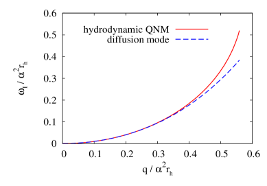
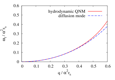
Figure 1: The dispersion relations for the electromagnetic hydrodynamic quasinormal modes of the rotating black string with $\mathfrak{m}=0$ for $a\alpha=0.2$ (left) and $a\alpha=0.5$ (right). The solid (red) lines show the numerical results, while the dashed (blue) lines are plots for the diffusion mode (47). Solid lines terminate at the indicated points, while the dashed lines extend to higher values of $q/\alpha^{2}r_{h}$. As expected, the analytical results (diffusion mode) are in good agreement with the numerical results (hydrodynamic QNM) just in the hydrodynamic limit ($\mathfrak{w}\ll 1$ and $\mathfrak{q}\ll 1$).

The behavior of the hydrodynamic QNM propagating along the perpendicular direction to the rotation, i.e., for which $\mathfrak{m}=0$, and for small rotation parameters $a$, is similar to the static case. In particular, there exist a saturation point, i.e., a maximum wavenumber value $\mathfrak{q}_{\mbox{\scriptsize{lim}}}$, beyond which the specific mode disappears (for more details see ref. [41], and for similar QNM emerging in other spacetimes, see ref. [51]). This implies that both of the solid lines in the graphs of figure 1 terminate at the largest values of the wavenumber $\mathfrak{q}=q/\alpha^{2}r_{h}$ showed in the figure. However, as the rotation parameter increases the point of saturation moves to higher wavenumber values, and finally, for some critical value of the rotation parameter $a_{c}$, it disappears and the mode extends to arbitrarily large values of $\mathfrak{q}$. The graphs of figure 2 exemplify this behavior. One can see that for $a\alpha=0.1$ the point of saturation occurs in $\mathfrak{q}\simeq 0.561$, and for $a\alpha=0.3$ in $\mathfrak{q}\simeq 0.595$. On the other hand, for $a\alpha=0.5$ and $a\alpha=0.7$ the point of saturation disappears and the purely damped dispersion relation extends continuously for higher values of $\mathfrak{q}$. A more detailed numerical analysis indicates the critical value $a\alpha=a_{c}\,\alpha=0.395$ as the limit where there still exists a saturation point (in $\mathfrak{q}\simeq 0.633$), but for $a\alpha\gtrsim 0.395$ the point of saturation no longer exists. This peculiar feature is still not well understood since the saturation point is outside the hydrodynamic limit and the analytical expressions are not valid in this region. However, we find a similar behavior in other physical systems, like the D3-D7’ model in the presence of a background magnetic field and at finite density [52]. In figure 2, we can see again a good agreement between all the analytical and numerical results in the hydrodynamic limit.

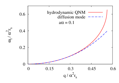
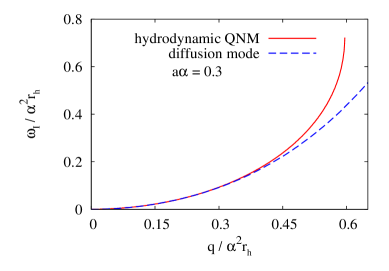
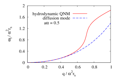
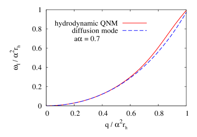
Figure 2: Dispersion relations for the special case of the hydrodynamic quasinormal mode with $\mathfrak{m}=0$ (purely damped). As in the static case, for $a\alpha=0.1$ and $a\alpha=0.3$ there is a saturation point beyond which the hydrodynamic QNM ceases to be purely damped, but for $a\alpha=0.5$ and $a\alpha=0.7$ the purely damped mode extends to higher values of $\mathfrak{q}$.

5.1.2 Wavemodes propagating along the rotation direction

We also analyzed the hydrodynamic quasinormal modes propagating along the rotation direction $\varphi$, i.e, modes with wave-vectors parallel to rotation direction, characterized by wavenumber of the form $\mathfrak{q}=0$ and $\mathfrak{m}\neq 0$. In this case, differently from the static case and differently from the rotating case for $\mathfrak{m}=0$, the dispersion relations have nonzero real and imaginary parts (see figure 3) for all wavenumber values. One of the reasons for the emergence of a non-zero real part for the frequency is the convective motion of the dual fluid with respect to the preferred rest frame introduced by the topology. Again we can see a satisfactory agreement between analytical and numerical results in the hydrodynamic regime.

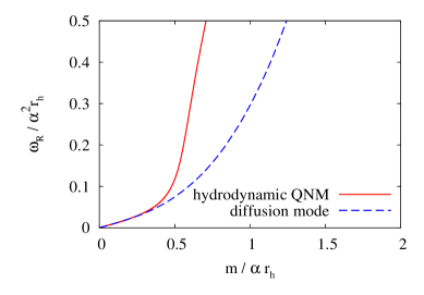
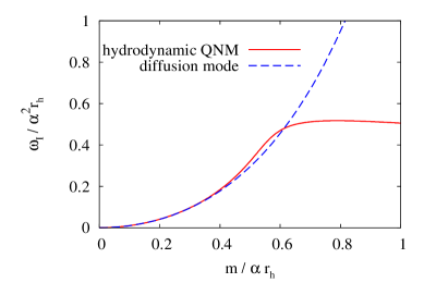
Figure 3: The dispersion relations for the electromagnetic hydrodynamic QNM of a rotating black string with $\mathfrak{q}=0$ and $a\alpha=0.1$. Both the real (left) and the imaginary (right) parts of the quasinormal frequency are shown. The solid lines correspond to the hydrodynamic quasinormal mode and the dashed lines correspond to the diffusion mode (47). Again, we can see the agreement between numerical and analytical results in the hydrodynamic limit $(\mathfrak{w},\mathfrak{m})\rightarrow 0$, as expected.

5.2 Purely damped quasinormal modes - slow rotation

Purely damped non-hydrodynamic QNM are also found in the electromagnetic perturbations of rotating black strings. These modes arise both in the longitudinal and in the transverse sectors for perturbations propagating only along the perpendicular direction to the rotation (with $\mathfrak{m}=0$). The behavior of the dispersion relations of such modes is similar to static case [41]. The purely damped modes of the static AdS black hole are found only for small values of wavenumber $\mathfrak{q}$ (for $\mathfrak{m}=0$), and extend to high values of the frequencies in a tower of modes with equally spaced imaginary frequencies. However, the higher is the frequency, the smaller is the domain of values of $\mathfrak{q}$ where the modes exist. As obtained from the numerical study, the behavior of the purely damped modes of the rotating black strings strongly depends on the value of the rotation parameter $a$. These modes are not equally spaced in the frequency, and disappear above some critical value of the frequency, which depends on the rotation parameter. On the other hand, for large values of $a$, it appears a different class of purely damped modes which extend to high values of the wavenumber. All of these modes were studied in some detail, as shown in figures 4 and 5.

Figure 4 shows some of the typical results found, where we can see that at small values of the $a$, the purely damped modes have a standard behavior that is repeated for different values of the rotation parameter. We discuss here the behavior of dispersion relations for $a\alpha=0.1$ (center panels of figure 4). For the other values of the $a$ the analysis is similar.

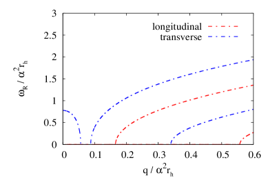
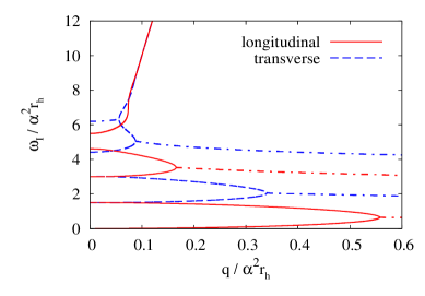
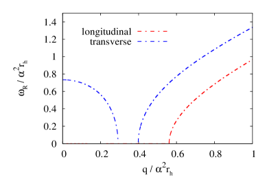
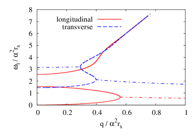
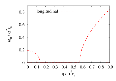
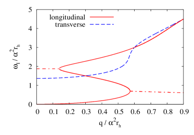
Figure 4: The dispersion relations for the purely damped QNM are shown by the solid and dashed lines (plots on the right) for different values of the rotation parameter. From top to bottom, we have $a\alpha=0.01$, $a\alpha=0.1$ and $a\alpha=0.2$. For completeness, ordinary modes (dot-dashed lines) connected to the purely damped ones are also shown. Real (imaginary) parts of the frequencies of these modes are shown in the graphs on the left (right) hand side.

For $a\alpha=0.1$, we found just three longitudinal purely damped modes (red solid lines), where the hydrodynamic QNM and the first purely damped non-hydrodynamic mode do not show new features in comparison to the static case [41]. There is a saturation point in $\mathfrak{q}\equiv\mathfrak{q}_{\scriptscriptstyle{lim}}\sim 0.56$, where the frequencies of the two modes coincide, and for wavenumber values larger than $\mathfrak{q}_{\scriptscriptstyle{lim}}$ the purely damped modes no longer exist. As in the static case, for larger values of $\mathfrak{q}$ there is an ordinary QNM, i.e., a mode whose real and imaginary parts of the frequency are both nonzero, and that starts exactly at the saturation point (see the dot-dashed lines in figure 4). On the other hand, the third longitudinal mode does not present saturation point and, for all values of the $\mathfrak{q}$ we have investigated, it remains purely damped. Differently from the static case where it exists an infinite tower of purely damped modes for small wavenumber values, no other purely damped longitudinal mode was found. The imaginary part of the frequency of the last purely damped longitudinal mode found grows very fast with the wavenumber, meaning that such modes are highly damped. This is a particular characteristic of the purely damped QNM of rotating black strings.

For transverse perturbations, and with $a\alpha=0.1$, we also find just three purely damped modes (dashed blue lines in figure 4). The first mode, similar to the static case, begins at $\mathfrak{q}=0$, extends to $\mathfrak{q}\sim 0.39$, disappearing for $\mathfrak{q}>0.39$. The second purely damped mode is present only in the region $0.29\lesssim\mathfrak{q}\lesssim 0.39$, and it meets the first mode at $\mathfrak{q}\sim 0.39$. Finally, the third purely damped QNM is identified as belonging to the region $\mathfrak{q}\gtrsim 0.29$ and, as the wavenumber increases, this purely damped mode extends to higher values of the frequency. For the values of $\mathfrak{q}$ considered in the analysis, the third mode does not present real part of the quasinormal frequency. It is also seen that the third transverse mode grows fast with the wavenumber, merging with the third longitudinal mode in the limit of high wavenumbers. As seen in the second graph in the right panel of figure 4, for wavenumber values lower than the saturation point, the behavior of the first purely damped mode is similar to the static case. However, the second purely damped mode does not exists for $\mathfrak{q}\lesssim 0.29$. Moreover, another important difference when compared to the static case is the presence of an ordinary mode, a mode whose frequency has nonzero real and imaginary parts in the region of small wavenumbers ($0\leq\mathfrak{q}\lesssim 0.29$). In fact, this kind of ordinary mode is present only for small wavenumbers, where the imaginary part of the frequency is approximately a constant, and it touches the last purely damped mode found for each sufficiently small given value of the rotation parameter.

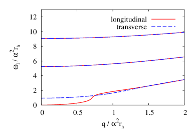
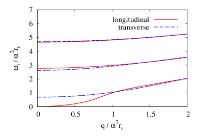
Figure 5: Dispersion relations of a special kind of purely damped electromagnetic QNM of the rotating black string for two different values of the rotation parameter: $a\alpha=0.5$ (left) and $a\alpha=0.7$ (right). These are special modes in the sense that they are not found for small rotation, neither have similar counterparts in the static case. See also table 1.

	$a\alpha=0.5$		$a\alpha=0.7$
$n_{\scriptscriptstyle{S}}$	Longitudinal	Transverse	Longitudinal	Transverse
0	0	0.940071	0	0.677287
1	5.24188	5.23989	2.76648	2.61773
2	9.06564	9.06564	4.65369	4.68590
3	12.8122	12.8122	6.60254	6.59832
4	16.5355	16.5355	8.51922	8.51901

Table 1: Five different overtones of purely damped QNM for longitudinal and transverse electromagnetic perturbation sectors with $a\alpha=0.5$ and $a\alpha=0.7$, and with $\mathfrak{q}=\mathfrak{m}=0$. See also figure 5.

5.3 Purely damped quasinormal modes - fast rotation

It is worth saying that for small nonzero values of the rotation parameter it was not found other purely damped modes in any region of the spectrum (for finite values of frequencies and wavenumbers, with $\mathfrak{m}=0$). Meanwhile, for higher values of the rotation parameter we have also found a special series of purely damped modes, both for longitudinal and transverse perturbation sectors, which do not present saturation points. They are special modes in the sense that they are not found for small values of the rotation parameter, neither have similar counterparts in the static case. We show a few of such modes for $a\alpha=0.5$ and $a\alpha=0.7$ in figure 5. We note that, for high values of the rotation parameter, the longitudinal and transverse quasinormal frequencies have very close values. These results indicate the isospectrality of the purely damped modes in high rotation. The same effect seems to happen for the other class of purely damped modes found in the slow rotating case, namely, the modes that exist at high wavenumbers and high frequencies (cf. the upper lines in figure 4). To confirm the isospectrality of the modes of figure 5, we list the values of the quasinormal frequencies for the first five of these modes calculated at zero wavenumbers ($\mathfrak{q}=\mathfrak{m}=0$) in table 1.

5.4 Ordinary quasinormal modes

As in the case of static black holes, the electromagnetic perturbations of rotating black strings also present a group of ordinary (or regular) QNM characterized by having nonzero frequencies (both real and imaginary parts) in the zero wavenumber limit, $\mathfrak{m}\rightarrow 0$ and $\mathfrak{q}\rightarrow 0$. Here we investigate these modes for longitudinal and transverse sectors considering a few different values of the rotation parameter ($a\alpha=0.1,\;0.2,\;0.5$ and $0.7$).

In table 2 we present the quasinormal frequencies for the first four transverse and longitudinal regular modes calculated with $a\alpha=0.1$ and $\mathfrak{q}=\mathfrak{m}=0$.

	Longitudinal		Transverse
$n$	$\quad\;\;\mathfrak{w}_{\scriptscriptstyle{R}}\quad\;\;$	$\quad\;\;\mathfrak{w}_{\scriptscriptstyle{I}}\quad\;\;$	$\quad\;\;\mathfrak{w}_{\scriptscriptstyle{R}}\quad\;\;$	$\quad\;\;\mathfrak{w}_{\scriptscriptstyle{I}}\quad\;\;$
1	1.49581	4.13330	2.25027	5.15701
2	2.98987	6.21144	3.71623	7.28524
3	4.43191	8.37247	5.13900	9.46958
4	5.83910	10.5744	6.53342	11.6853

Table 2: Ordinary QNM for longitudinal and transverse electromagnetic perturbations with $a\alpha=0.1$ and $\mathfrak{q}=\mathfrak{m}=0$.

In figure 6 we plot the dispersion relations of the first ($n=1$) longitudinal and transverse ordinary QNM for $a\alpha=0.1$. The graphs on the left hand side of the figure show real parts of the frequency and the graphs on the right hand side show the imaginary parts of the frequency. It can be seen that, for both perturbation sectors, the imaginary parts of the frequency are not symmetric with respect to the wavenumber $\mathfrak{m}$. It is noteworthy that the symmetry with respect to the wavenumber $\mathfrak{q}$ is preserved, so we plot only the positive values of wavenumber $\mathfrak{q}$.

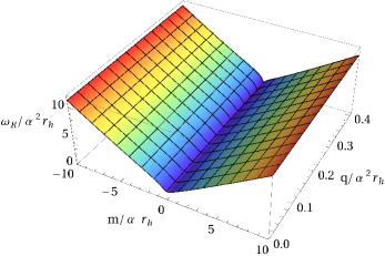
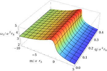
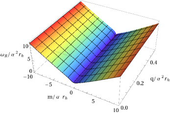
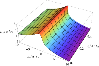
Figure 6: Dispersion relations of the first ($n=1$) longitudinal (top) and transverse (bottom) ordinary QNM in the case $a\alpha=0.1$. The real parts of the frequency are in the graphs on the left, and the imaginary parts of the frequency are in the graphs on the right.

It is seen that the imaginary parts of the frequency decrease with the wavenumber $\mathfrak{m}$, while the real parts increase. The imaginary parts of the frequency decrease faster for positive values of the wavenumber $\mathfrak{m}$ than for negative values. Although graphically the real parts of the frequency seem to be symmetric, the values of the frequency for symmetric values of $\mathfrak{m}$ are different. For example, the frequency of the longitudinal quasinormal mode at $(\mathfrak{q},\,\alpha\mathfrak{m})=(0.2,\,+6.0)$ is $\mathfrak{w}_{\scriptscriptstyle{R}}=6.76969$, while at $(\mathfrak{q},\,\alpha\mathfrak{m})=(0.2,\,-6.0)$ it is $\mathfrak{w}_{\scriptscriptstyle{R}}=7.34660$. The difference is easily understood as Doppler shift.

The quasinormal frequencies of a few ordinary modes found with $\mathfrak{q}=\mathfrak{m}=0$, for $a\alpha=0.2,\;0.5$ and $0.7$, are shown in table 3.

Longitudinal sector
	$a\alpha=0.2$		$a\alpha=0.5$		$a\alpha=0.7$
$\;\;n\;\;$	$\quad\;\;\mathfrak{w}_{\scriptscriptstyle{R}}\quad\;\;$	$\quad\;\;\mathfrak{w}_{\scriptscriptstyle{I}}\quad\;\;$	$\quad\;\;\mathfrak{w}_{\scriptscriptstyle{R}}\quad\;\;$	$\quad\;\;\mathfrak{w}_{\scriptscriptstyle{I}}\quad\;\;$	$\quad\;\;\mathfrak{w}_{\scriptscriptstyle{R}}\quad\;\;$	$\quad\;\;\mathfrak{w}_{\scriptscriptstyle{I}}\quad\;\;$
1	$1.89070$	3.83011	$0.698883$	1.41673	0.779558	1.28190
2	$3.37595$	6.00354	$2.26543$	3.90299	$2.70200$	4.68020
3	$4.79244$	8.28380	$3.95790$	6.85402	$4.80012$	8.31405
4	$6.17560$	10.6313	$5.67558$	9.83043	$6.91203$	11.9720
Transverse sector
	$a\alpha=0.2$		$a\alpha=0.5$		$a\alpha=0.7$
$\;\;n\;\;$	$\quad\;\;\mathfrak{w}_{\scriptscriptstyle{R}}\quad\;\;$	$\quad\;\;\mathfrak{w}_{\scriptscriptstyle{I}}\quad\;\;$	$\quad\;\;\mathfrak{w}_{\scriptscriptstyle{R}}\quad\;\;$	$\quad\;\;\mathfrak{w}_{\scriptscriptstyle{I}}\quad\;\;$	$\quad\;\;\mathfrak{w}_{\scriptscriptstyle{R}}\quad\;\;$	$\quad\;\;\mathfrak{w}_{\scriptscriptstyle{I}}\quad\;\;$
1	$1.11157$	2.82061	$1.49788$	2.52890	$1.66774$	2.89436
2	$2.64477$	4.89856	$3.10140$	5.37862	$3.74734$	6.49058
3	$4.09020$	7.13378	$4.81471$	8.33942	$5.85513$	10.1414
4	$5.48647$	9.45034	$6.53797$	11.3241	$7.96969$	13.8039

Table 3: The longitudinal and the transverse frequencies of the first four ordinary QNM for $a\alpha=0.2$, $a\alpha=0.5$, and $a\alpha=0.7$, calculated with $\mathfrak{q}=\mathfrak{m}=0$.

The dispersion relations for these quasinormal modes present similar behavior as those showed in figure 6, and therefore they will not be presented here.

From the point of view of AdS/CFT correspondence, the rotating black string studied here is holographically dual to a CFT plasma moving with respect to the preferred rest frame introduced by the topology. Therefore, an observer at AdS boundary (CFT side) can see a wave propagating along the direction of the motion of the plasma (with wavenumber $+\mathfrak{m}$), and another wave propagating along the opposite direction (with wavenumber $-\mathfrak{m}$). This justifies the fact that the numerical results for the frequency show a symmetry breaking with respect to the wavenumber $\mathfrak{m}$. In fact, this break of symmetry happens in both the longitudinal and the transverse sectors of the electromagnetic fluctuations, and it is due to kinematic effects like the Doppler shift.

The overall effect of the rotation in the quasinormal frequencies of AdS black strings can be analyzed through the graphs of figure 7. We have chosen to show here the fundamental quasinormal modes for each perturbation sector because these modes are important from the point of view of AdS/CFT correspondence. The graphs of figure 7 show the evolution of the frequency as a function of the rotation parameter for fixed wavenumber ($\mathfrak{m}=0$ and $\mathfrak{q}=0.1$).

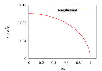
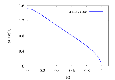
Figure 7: Imaginary parts of the quasinormal frequencies as a function of the rotation parameter with fixed wavenumber ($\mathfrak{m}=0$ and $\mathfrak{q}=0.1$). On the left, the longitudinal (hydrodynamic) mode and on the right the first transverse (purely damped) mode.

It is seen that the rotation implies in a contraction of the imaginary parts of the fundamental quasinormal frequencies for both perturbation sectors. Based on the AdS/CFT correspondence, this behavior means that the rotation implies in a dilation of the thermalization time of the dual CFT plasma, in agreement with our analytical results (cf. eq. (50)).

6 Final comments and conclusion

In this work the previous study of electromagnetic perturbations of static AdS black holes was extended to AdS rotating black strings [34]. The electromagnetic perturbation equations were obtained in a covariant form and the resulting expressions imply that the QNM frequencies and wavenumbers of the rotating black string are related to the QNM frequencies and wavenumbers of the static black string through simple expressions (cf. equations (45)).

The longitudinal hydrodynamic quasinormal mode of the electromagnetic perturbations of the rotating black strings was found numerically, by directly solving the perturbation equations, and analytically through relations (45). Differently from the static case, this diffusive mode has quasinormal frequency with nonzero real part, which can be interpreted as a convection term that emerges due to the motion of fluid in relation to the preferred inertial frame introduced by the topology. The hydrodynamic quasinormal mode presents a new diffusion coefficient for the corresponding fluid, $D=\bar{D}/\gamma$, that depends on the rotation parameter and implies a contraction of the imaginary parts of the frequencies.

The non-hydrodynamic QNM were also obtained and some of their dispersion relations have been presented. In comparison to the static case, the main new characteristic is a break of symmetry in the dispersion relations under inversion of the wavenumber component in the direction of the rotation ($\mathfrak{m}\rightarrow-\mathfrak{m}$), while the symmetry with respect to the wavenumber perpendicular to the rotation direction ($\mathfrak{q}$) is preserved. This symmetry breaking in the rotation direction can be associated to Doppler shifts of the frequencies and wavenumbers.

Both analytically and numerically we observed that rotation implies in a decreasing of the values of the imaginary parts of the quasinormal frequencies for both of the perturbation sectors, and hence, following the AdS/CFT duality, the rotation implies in dilation of the thermalization times of the CFT plasma.

We have also found a special class of electromagnetic purely damped modes of the rotating black string which exists only for modes propagating along the perpendicular direction to the rotation ($\mathfrak{m}=0$). More study is necessary in order to find possible interpretations of this special family of quasinormal modes.

7 Acknowledgments

This work is partly supported by Fundação de Amparo à Pesquisa do Estado de São Paulo (FAPESP, Brazil). VTZ thanks Conselho Nacional de Desenvolvimento Científico e Tecnológico (CNPq, Brazil) for financial support.

References

- [1] J. M. Maldacena, The large N limit of superconformal field theories and supergravity, Adv. Theor. Math. Phys. 2 (1998) 231 [Int. J. Theor. Phys. 38 (1999) 1113] [hep-th/9711200].
- [2] E. Witten, Anti-de Sitter space and holography, Adv. Theor. Math. Phys. 2 (1998) 253 [hep-th/9802150].
- [3] S. S. Gubser, I. R. Klebanov and A. M. Polyakov, Gauge theory correlators from non-critical string theory, Phys. Lett. B 428 (1998) 105 [hep-th/9802109].
- [4] O. Aharony, S. S. Gubser, J. M. Maldacena, H. Ooguri and Y. Oz, Large N field theories, string theory and gravity, Phys. Rept. 323 (2000) 183 [hep-th/9905111].
- [5] H. Boschi-Filho and N. R. F. Braga, Gauge/string duality and hadronic physics, Braz. J. Phys. 37 (2007) 567 [hep-th/0604091].
- [6] D. T. Son and A. O. Starinets, Viscosity, black holes, and quantum field theory, Ann. Rev. Nucl. Part. Sci. 57 (2007) 95 [arXiv:0704.0240].
- [7] S. S. Gubser, Heavy ion collisions and black hole dynamics, Gen. Rel. Grav. 39 (2007) 1533 [Int. J. Mod. Phys. D 17 (2008) 673].
- [8] J. Erdmenger, N. Evans, I. Kirsch and E. Threlfall, Mesons in gauge/gravity duals, Eur. Phys. J. A 35 (2008) 81 [arXiv:0711.4467].
- [9] E. Iancu, Partons and jets in a strongly-coupled plasma from AdS/CFT, Acta Phys. Polon. B 39 (2008) 3213 [arXiv:0812.0500].
- [10] R. C. Myers and S. E. Vazquez, Quark Soup al dente: Applied Superstring Theory, Class. Quant. Grav. 25 (2008) 114008 [arXiv:0804.2423].
- [11] V. E. Hubeny and M. Rangamani, A holographic view on physics out of equilibrium, Adv. High Energy Phys. 2010 (2010) 297916 [arXiv:1006.3675].
- [12] C. P. Herzog, Lectures on holographic superfluidity and superconductivity, J. Phys. A 42 (2009) 343001 [arXiv:0904.1975].
- [13] S. A. Hartnoll, Lectures on holographic methods for condensed matter physics, Class. Quant. Grav. 26 (2009) 224002 [arXiv:0903.3246].
- [14] J. McGreevy, Holographic duality with a view toward many-body physics, Adv. High Energy Phys. 2010 (2010) 723105 [arXiv:0909.0518].
- [15] S. S. Gubser, Breaking an Abelian gauge symmetry near a black hole horizon, Phys. Rev. D 78 (2008) 065034 [arXiv:0801.2977].
- [16] S. A. Hartnoll, C. P. Herzog and G. T. Horowitz, Building a Holographic Superconductor, Phys. Rev. Lett. 101 (2008) 031601 [arXiv:0803.3295].
- [17] S. A. Hartnoll, C. P. Herzog and G. T. Horowitz, Holographic Superconductors, JHEP 12 (2008) 015 [arXiv:0810.1563].
- [18] K. S. Thorne, R. H. Price and D. A. Macdonald, Black holes: the membrane paradigm, Yale Univ. Press, New Haven, U.S.A. (1986).
- [19] M. Parikh and F. Wilczek, An action for black hole membranes, Phys. Rev. D 58 (1998) 064011 [gr-qc/9712077].
- [20] P. Kovtun, D. T. Son and A. O. Starinets, Holography and hydrodynamics: diffusion on stretched horizons, JHEP 10 (2003) 064 [hep-th/0309213].
- [21] M. Fujita, Non-equilibrium thermodynamics near the horizon and holography, JHEP 10 (2008) 031 [arXiv:0712.2289]
- [22] N. Iqbal and H. Liu, Universality of the hydrodynamic limit in AdS/CFT and the membrane paradigm, Phys. Rev. D 79 (2009) 025023 [arXiv:0809.3808].
- [23] S. Bhattacharyya, V. EHubeny, S. Minwalla and M. Rangamani, Nonlinear fluid dynamics from gravity, JHEP 02 (2008) 045 [arXiv:0712.2456].
- [24] S. Bhattacharyya, R. Loganayagam, S. Minwalla, S. Nampuri, S. P. Trivedi and S. R. Wadia, Forced fluid dynamics from gravity, JHEP 02 (2009) 018 [arXiv:0806.0006].
- [25] I. Bredberg, C. Keeler, V. Lysov and A. Strominger, Wilsonian approach to fluid/gravity duality, JHEP 03 (2011) 141 [arXiv:1006.1902].
- [26] I. Bredberg, C. Keeler, V. Lysov and A. Strominger, From Navier-Stokes to Einstein, JHEP 07 (2012) 146 [arXiv:1101.2451].
- [27] P. Kovtun, D. T. Son, and A. O. Starinets, Viscosity in strongly interacting quantum field theories from black hole physics, Phys. Rev. Lett. 94 (2005) 111601.
- [28] M. M. Caldarelli, O. J. C. Dias, R. Emparan, D. Klemm, Black Holes as Lumps of Fluid, JHEP 04 (2009) 024 [arXiv:0811.2381].
- [29] J.P.S. Lemos,Two-dimensional black holes and planar general relativity, Class.Quant.Grav., 12 (1995) 1081 [gr-qc/9407024].
- [30] C. G. Huang and C. B. Liang, A torus-like black hole, Phys. Lett. A 201 (1995) 27.
- [31] R. -G. Cai and Y. -Z. Zhang, Black plane solutions in four-dimensional spacetimes, Phys. Rev. D 54 (1996) 4891 [gr-qc/9609065].
- [32] D. R. Brill, J. Louko and P. Peldan, Thermodynamics of (3+1)-dimensional black holes with toroidal or higher genus horizons, Phys. Rev. D 56 (1997) 3600 [gr-qc/9705012].
- [33] J. Stachel, Globally stationary but locally static space-times: A gravitational analog of the Aharonov-Bohm effect, Phys. Rev. D 26 (1982) 1281.
- [34] J. P. S. Lemos, Cylindrical black hole in general relativity, Phys. Lett. B 353 (1995) 46 [gr-qc/9404041].
- [35] E. Berti, V. Cardoso and A. O. Starinets, Quasinormal modes of black holes and black branes, Class. Quant. Grav. 26 (2009) 163001 [arXiv:0905.2975].
- [36] R. A. Konoplya and A. Zhidenko, Quasinormal modes of black holes: from astrophysics to string theory, Rev. Mod. Phys. 83 (2011) 793 [arXiv:1102.4014].
- [37] G. T. Horowitz and V. E. Hubeny, Quasinormal modes of AdS black holes and the approach to thermal equilibrium, Phys. Rev. D 62 (2000) 024027 [hep-th/9909056].
- [38] J. P. S. Lemos, Rotating toroidal black holes in anti-de Sitter space-times and their properties, 2000, gr-qc/0011092.
- [39] J. P. S. Lemos and V. T. Zanchin, Rotating charged black string and three-dimensional black holes, Phys. Rev. D 54 (1996) 3840 [hep-th/9511188].
- [40] S. Bhattacharyya, R. Loganayagam, I. Mandal, S. Minwalla, A. Sharma, Conformal Nonlinear Fluid Dynamics from Gravity in Arbitrary Dimensions, JHEP 12 (2008) 116 [arXiv:0809.4272].
- [41] A. S. Miranda, J. Morgan and V. T. Zanchin, Quasinormal modes of plane-symmetric black holes according to the AdS/CFT correspondence, JHEP 11 (2008) 030 [arXiv:0809.0297].
- [42] P. K. Kovtun and A. O. Starinets, Quasinormal modes and holography, Phys. Rev. D 72 (2005) 086009 [hep-th/0506184].
- [43] A. S. Miranda and V. T. Zanchin, Quasinormal modes of plane-symmetric anti-de Sitter black holes: A complete analysis of the gravitational perturbations, Phys. Rev. D 73 (2006) 064034 [gr-qc/0510066].
- [44] C. P. Herzog, The hydrodynamics of M-theory, JHEP 12 (2002) 026 [hep-th/0210126].
- [45] G. Policastro, D. T. Son and A. O. Starinets, From AdS/CFT correspondence to hydrodynamics, JHEP 09 (2002) 043 [hep-th/0205052].
- [46] G. Policastro, D. T. Son and A. O. Starinets, From AdS/CFT correspondence to hydrodynamics. II: Sound waves, JHEP 12 (2002) 054 [hep-th/0210220].
- [47] C. P. Herzog, The sound of M-theory, Phys. Rev. D 68 (2003) 024013 [hep-th/0302086].
- [48] R. Baier, P. Romatschke, D. T. Son, A. O. Starinets and M. A. Stephanov, Relativistic viscous hydrodynamics, conformal invariance, and holography, JHEP 04 (2008) 100 [arXiv:0712.2451].
- [49] M. Natsuume and T. Okamura, Causal hydrodynamics of gauge theory plasmas from AdS/CFT duality, Phys. Rev. D 77 (2008) 066014 [Erratum-ibid. D 78 (2008) 089902] [arXiv:0712.2916].
- [50] J. Morgan, V. Cardoso, A.S. Miranda, C. Molina, and V.T. Zanchin, Gravitational quasinormal modes of AdS black branes in d spacetime dimensions, JHEP 07 (2009) 117 [arXiv:0907.5011].
- [51] R. C. Myers, and M. C. Wapler, Transport Properties of Holographic Defects, JHEP 0812, 115 (2008), arXi:0811.0480 [hep-th].
- [52] N. Jokela, N. G. Lifschytz, and M. Lippert, Magnetic effects in a holographic Fermi-like liquid, JHEP 1205, 105 (2012), arXiv:1204.3914 [hep-th].