CENTRALITY-CONSTRAINED GRAPH EMBEDDING

Abstract

Visual rendering of graphs is a key task in the mapping of complex network data. Although most graph drawing algorithms emphasize aesthetic appeal, certain applications such as travel-time maps place more importance on visualization of structural network properties. The present paper advocates a graph embedding approach with centrality considerations to comply with node hierarchy. The problem is formulated as one of constrained multi-dimensional scaling (MDS), and it is solved via block coordinate descent iterations with successive approximations and guaranteed convergence to a KKT point. In addition, a regularization term enforcing graph smoothness is incorporated with the goal of reducing edge crossings. Experimental results demonstrate that the algorithm converges, and can be used to efficiently embed large graphs on the order of thousands of nodes.

Index Terms—  MDS, graph embedding, coordinate descent.

1 Introduction

Graphs offer a valuable means of encoding relational information between entities of complex systems, arising in modern communications, transportation and social networks, among others. Despite the abundance of network analysis techniques, information visualization is a powerful tool for capturing patterns that may not be apparent in large-scale systems. However, most visualization algorithms focus more on aesthetic appeal than the structural characteristics of the underlying data. Such network structure is captured through graph-theoretic notions such as node centrality and network cohesion.

The present paper deals with embedding graphs for visualization while adhering to the underlying node centrality structure. Centrality measures capture the relative importance of network nodes among their peers. Betweenness centrality for instance, describes the extent to which information is routed through a specific node by measuring the fraction of all shortest paths traversing this node; see e.g., [1, p. 89]. Other measures include closeness, eigenvalue, and degree centrality. To incorporate centrality using any of these metrics, an MDS (so-termed stress [2, Chap. 3]) criterion is adopted, under radial constraints that place nodes of higher centrality closer to the origin of the graph embedding. MDS seeks a low-dimensional depiction of high-dimensional data in which pairwise Euclidean distances between embedding coordinates are close (in a well-defined sense) to the dissimilarities between the original data points. Closeness criteria (a.k.a. stress costs) are generally non-convex, and the quest for global optimality is challenging because ordinary descent methods do not have optimality guarantees, and are sensitive to initialization. Successive approximation with global and convex upper bounds is used in [2, Chap. 8] to minimize the stress cost yielding near-optimal results.

The novel approach exploits the block separability inherent to the proposed model and adapts the coordinate descent algorithm to determine the optimal embedding. Edge crossings are minimized by regularizing the cost with a smoothness promoting term weighted by a tuning parameter. Smoothness encourages nodes that share an edge to lie closer to each other in the embedding. As a result, the length and hence the number of edge crossings in the network visualization is markedly reduced. In addition, the regularization term offers the benefit of incorporating the underlying network topology when the dissimilarities considered are not graph-theoretic e.g., Euclidean distances between feature vectors associated with each node. Moreover, numerical tests illustrate that judicious selection of the tuning parameter results in fewer block coordinate descent iterations, which in turn yields a visually appealing embedding.

To place the present work in context, a prior approach iteratively minimizes a weighted stress function with iteration-dependent weights chosen to incorporate radial constraints [3]. However, it is limited to graph-theoretic dissimilarities, and offers no convergence guarantees. A heuristic algorithm for network visualization uses the $k$-core decomposition to hierarchically place nodes within “onion-like” concentric shells [4]. Although effective for large-scale networks, it has no optimality associated with it, and is limited to visualization only in $2$ dimensions. The proposed approach scales well for large networks under a well-defined optimality criterion with a convergence guarantee.

2 Model and Problem Statement

Consider a network represented by an undirected graph $\mathcal{G}=(\mathcal{V},\mathcal{E})$, where $\mathcal{E}$ denotes the set of edges, and $\mathcal{V}$ the set of vertices with cardinality $|\mathcal{V}|=N$. Let $\delta_{ij}$ denote the pairwise dissimilarity (edge weight) between any two nodes $i$ and $j$. Given the set $\{\delta_{ij}\}$ and the prescribed embedding dimension $p$, the graph embedding task amounts to finding $p\times 1$ vectors $\left\{{\mathbf{x}}_{i}\right\}_{i=1}^{N}$ so that the embedding coordinates ${\mathbf{x}}_{i}$ and ${\mathbf{x}}_{j}$ satisfy $\|{\mathbf{x}}_{i}-{\mathbf{x}}_{j}\|_{2}\approx\delta_{ij}$.

With $\delta_{ij}=\delta_{ji}$, it suffices to know $\{\{\delta_{ij}\}_{j=1}^{N}\}_{i=j+1}^{N}$, or, be possible to determine them from $\mathcal{G}$. Most visualization schemes assign $\delta_{ij}$ to the shortest path distance between nodes $i$ and $j$. In this work, the Euclidean commute-time distance (ECTD) is adopted because it decreases as the number of shortest paths between node pairs increases [5]. This is more reasonable since having multiple shortest paths between node pairs endows them with a higher level of accessibility by e.g., a random walker on the graph.

MDS amounts to solving the following problem:

$$(\text{P}0)\;\;\;\;\left\{\hat{{\mathbf{x}}}_{i}\right\}_{i=1}^{N}=\underset{{\mathbf{x}}_{1},\dots,{\mathbf{x}}_{N}}{\operatorname{arg\,min}}\text{ }\frac{1}{2}\sum_{i=1}^{N}\sum_{j=1}^{N}[\left\|\mathbf{x}_{i}-\mathbf{x}_{j}\right\|_{2}-\delta_{ij}]^{2}.$$ (1)

Turning attention to node centralities $\{c_{i}\}_{i=1}^{N}$, those can be obtained using a number of algorithms [1, Chap. 4]. Centrality structure will be imposed on (1) by constraining ${\mathbf{x}}_{i}$ to have a centrality-dependent radial distance $f(c_{i})$, where $f(.)$ is a monotone decreasing function. The resulting constrained optimization problem now becomes

$$(\text{P}1)\;\;\;\;\left\{\hat{{\mathbf{x}}}_{i}\right\}_{i=1}^{N}=\underset{{\mathbf{x}}_{1},\dots,{\mathbf{x}}_{N}}{\operatorname{arg\,min}} \frac{1}{2}\sum\limits_{i=1}^{N}\sum\limits_{j=1}^{N}\left[\left\|\mathbf{x}_{i}-\mathbf{x}_{j}\right\|_{2}-\delta_{ij}\right]^{2}$$

s. to $$\left\|\mathbf{x}_{i}\right\|_{2}=f(c_{i}),\text{ }i=1,\dots,N.$$ (2)

Although $\text{P}0$ is non-convex, standard solvers rely on gradient descent iterations but have no guarantees of convergence to the global optima [6]. Lack of convexity is exacerbated in $\text{P}1$ by the non-convex constraint set rendering its solution even more challenging than that of $\text{P}0$. However, considering a single embedding vector ${\mathbf{x}}_{i}$, and fixing the rest $\{{\mathbf{x}}_{j}\}_{j\neq i}$, the constraint set simplifies to $\|{\mathbf{x}}_{i}\|_{2}=f(c_{i})$, for which an appropriate relaxation can be sought. Key to the algorithm proposed next lies in this inherent decoupling of the centrality constraints.

3 BCD with successive approximations

By exploiting the separable nature of the cost as well as the norm constraints in (2), block coordinate descent (BCD) will be adopted in this section to arrive at a solution approaching the global optimum. To this end, the centering constraint $\sum_{i=1}^{N}{\mathbf{x}}_{i}={\bf 0}$, typically invoked to fix the inherent translation ambiguity, will be dropped first so that the problem remains decoupled across nodes. The effect of this relaxation can be compensated for by computing the centroid of the solution of (2), and subtracting it from each coordinate. The $N$ equality norm constraints are also relaxed to $\|{\mathbf{x}}_{i}\|_{2}\leq f(c_{i})$. Although the entire constraint set is non-convex, each relaxed constraint is a convex and closed Euclidean ball with respect to each node in the network.

Let ${\mathbf{x}}_{i}^{r}$ denote the minimizer of the optimization problem over block $i$, when the remaining blocks $\left\{{\mathbf{x}}_{j}\right\}_{j\neq i}$ are fixed during the BCD iteration $r$. By fixing the blocks $\left\{{\mathbf{x}}_{j}\right\}_{j\neq i}$ to their values from the most recent iterations, the sought embedding is obtained as

$$\left\{\hat{{\mathbf{x}}}_{i}\right\}_{i=1}^{N}=\underset{\left\{{\mathbf{x}}_{i}:\left\|\mathbf{x}_{i}\right\|_{2}\leq f(c_{i})\right\}}{\operatorname{arg\,min}}\frac{1}{2}\sum\limits_{i=1}^{N}\sum\limits_{j=1}^{N}\left[\left\|\mathbf{x}_{i}-\mathbf{x}_{j}\right\|_{2}-\delta_{ij}\right]^{2}$$ (3)

or equivalently as

$$\underset{\left\{{\mathbf{x}}_{i}:\left\|\mathbf{x}_{i}\right\|_{2}\leq f(c_{i})\right\}}{\arg\min}\frac{(N-1)}{2}\|{\mathbf{x}}_{i}\|_{2}^{2}-{\mathbf{x}}_{i}^{T}(\sum\limits_{j<i}{\mathbf{x}}_{j}^{r}+\sum\limits_{j>i}{\mathbf{x}}_{j}^{r-1})$$

$$-\sum\limits_{j<i}\delta_{ij}\|{\mathbf{x}}_{i}-{\mathbf{x}}_{j}^{r}\|_{2}-\sum\limits_{j>i}\delta_{ij}\|{\mathbf{x}}_{i}-{\mathbf{x}}_{j}^{r-1}\|_{2}$$ (4)

where $\sum\limits_{j<i}(.):=\sum\limits_{j=1}^{i-1}(.)$ and $\sum\limits_{j>i}(.):=\sum\limits_{j=i+1}^{N}(.)$. With the last two sums in (3) being non-convex and non-smooth, convergence of the BCD algorithm cannot be guaranteed [7, p. 272]. Moreover, it is desired to have each per-iteration subproblem solvable to global optimality, in closed form and at a minimum computational cost. The proposed approach seeks a global upper bound of the objective with the desirable properties of smoothness and convexity. To this end, consider the function $\Psi({\mathbf{x}}_{i}):=\psi_{1}({\mathbf{x}}_{i})-\psi_{2}({\mathbf{x}}_{i})$, where

$$\psi_{1}({\mathbf{x}}_{i}):=\frac{(N-1)}{2}\|{\mathbf{x}}_{i}\|_{2}^{2}-{\mathbf{x}}_{i}^{T}(\sum\limits_{j<i}{\mathbf{x}}_{j}^{r}+\sum\limits_{j>i}{\mathbf{x}}_{j}^{r-1})$$ (5)

and

$$\psi_{2}({\mathbf{x}}_{i}):=\sum\limits_{j<i}\delta_{ij}\|{\mathbf{x}}_{i}-{\mathbf{x}}_{j}^{r}\|_{2}+\sum\limits_{j>i}\delta_{ij}\|{\mathbf{x}}_{i}-{\mathbf{x}}_{j}^{r-1}\|_{2}.$$ (6)

Note that $\psi_{1}({\mathbf{x}}_{i})$ is a convex quadratic function, and that $\psi_{2}({\mathbf{x}}_{i})$ is convex (with respect to ${\mathbf{x}}_{i}$) but non-differentiable. The first-order approximation of (6) at any point in its domain is a global under-estimate of $\psi_{2}({\mathbf{x}}_{i})$. Despite the non-smoothness at some points, such a lower bound can always be established using its subdifferential. As a consequence of the convexity of $\psi_{2}({\mathbf{x}}_{i})$, it holds that [7, p. 731]

$$\psi_{2}({\mathbf{x}})\geq\psi_{2}({\mathbf{x}}_{0})+\mathbf{g}^{T}({\mathbf{x}}_{0})({\mathbf{x}}-{\mathbf{x}}_{0}),\forall{\mathbf{x}}\in\text{dom}(\psi_{2})$$ (7)

where $\mathbf{g}({\mathbf{x}})\in\partial\psi_{2}({\mathbf{x}})$ is a subgradient within the subdifferential set, $\partial\psi_{2}({\mathbf{x}})$ of $\psi_{2}({\mathbf{x}})$. The subdifferential of $\|{\mathbf{x}}_{i}-{\mathbf{x}}_{j}\|_{2}$ with respect to ${\mathbf{x}}_{i}$ is given by

$$\partial_{{\mathbf{x}}_{i}}\|{\mathbf{x}}_{i}-{\mathbf{x}}_{j}\|_{2}=\begin{cases}\frac{{\mathbf{x}}_{i}-{\mathbf{x}}_{j}}{\|{\mathbf{x}}_{i}-{\mathbf{x}}_{j}\|_{2}},&\text{ if }{\mathbf{x}}_{i}\neq{\mathbf{x}}_{j}\\ \mathbf{y}\in\mathbb{R}^{p}:\text{ }\|\mathbf{y}\|_{2}\leq 1,&\text{ otherwise }\end{cases}$$ (8)

which implies that

$$\partial_{{\mathbf{x}}_{i}}\psi_{2}({\mathbf{x}}_{i})=\sum\limits_{j=1}^{N}\delta_{ij}\partial_{{\mathbf{x}}_{i}}\|{\mathbf{x}}_{i}-{\mathbf{x}}_{j}\|_{2}.$$ (9)

Using (7), it is possible to lower bound (6) by

$$\psi_{2}^{\prime}({\mathbf{x}}_{i},{\mathbf{x}}_{0})=\sum\limits_{j<i}\delta_{ij}\left[\|{\mathbf{x}}_{0}-{\mathbf{x}}_{j}^{r}\|_{2}+(\mathbf{g}_{j}^{r})^{T}({\mathbf{x}}_{0})({\mathbf{x}}_{i}-{\mathbf{x}}_{0})\right]$$

$$+\sum\limits_{j>i}\delta_{ij}\left[\|{\mathbf{x}}_{0}-{\mathbf{x}}_{j}^{r-1}\|_{2}+(\mathbf{g}_{j}^{r-1})^{T}({\mathbf{x}}_{0})({\mathbf{x}}_{i}-{\mathbf{x}}_{0})\right].$$ (10)

Consider now $\Phi({\mathbf{x}}_{i},{\mathbf{x}}_{0}):=\psi_{1}({\mathbf{x}}_{i})-\psi_{2}^{\prime}({\mathbf{x}}_{i},{\mathbf{x}}_{0})$, and note that $\Phi({\mathbf{x}}_{i},{\mathbf{x}}_{0})$ is convex and upper bounds globally the cost in (3). The proposed BCD algorithm involves successive approximations using (3), and yields the following QCQP for each block

$$(\text{P}2)\quad\quad\underset{\left\{{\mathbf{x}}_{i}:\left\|\mathbf{x}_{i}\right\|_{2}\leq f(c_{i})\right\}}{\operatorname{arg\,min}}\Phi({\mathbf{x}}_{i},{\mathbf{x}}_{0}).$$ (11)

For convergence, ${\mathbf{x}}_{0}$ must be selected to satisfy the following conditions [8]:

$$\Phi({\mathbf{x}}_{0},{\mathbf{x}}_{0}) = \Psi({\mathbf{x}}_{0}),\quad\forall{\mathbf{x}}_{0}\in\mathcal{C},\forall i$$ (12a)

$$\Phi({\mathbf{x}}_{i},{\mathbf{x}}_{0}) \geq \Psi({\mathbf{x}}_{i}),\quad\|{\mathbf{x}}_{i}\|_{2}\leq f(c_{i}),\forall i$$ (12b)

where $\mathcal{C}:=\bigcup_{i=1}^{N}\left\{{\mathbf{x}}_{i}:\|{\mathbf{x}}_{i}\|_{2}\leq f(c_{i})\right\}$. In addition, $\Phi({\mathbf{x}}_{i},{\mathbf{x}}_{0})$ must be continuous in $({\mathbf{x}}_{i},{\mathbf{x}}_{0})$. Upon selecting ${\mathbf{x}}_{0}={\mathbf{x}}_{i}^{r-1}$, the iterate ${\mathbf{x}}_{i}^{r-1}$ satisfies (12a) and (12b). Taking successive approximations around ${\mathbf{x}}_{i}^{r-1}$ in $\text{P}2$, ensures the uniqueness of

$${\mathbf{x}}_{i}^{r} =\underset{\left\{{\mathbf{x}}_{i}:\left\|\mathbf{x}_{i}\right\|_{2}\leq f(c_{i})\right\}}{\operatorname{arg\,min}}\frac{(N-1)}{2}{\mathbf{x}}_{i}^{T}{\mathbf{x}}_{i}$$ (13)

$$-{\mathbf{x}}_{i}^{T}[\sum\limits_{j<i}({\mathbf{x}}_{j}^{r}+\delta_{ij}\mathbf{g}_{j}^{r}({\mathbf{x}}_{i}^{r-1}))$$

$$+\sum\limits_{j>i}({\mathbf{x}}_{j}^{r-1}+\delta_{ij}\mathbf{g}_{j}^{r-1}({\mathbf{x}}_{i}^{r-1}))]$$

Solving (13) amounts to obtaining the solution of the unconstrained QP, $({\mathbf{x}}_{i}^{*})^{r}$, and projecting it onto $\left\{{\mathbf{x}}_{i}:\left\|\mathbf{x}_{i}\right\|_{2}\leq f(c_{i})\right\}$; that is,

$${\mathbf{x}}_{i}^{r}=\begin{cases}\frac{({\mathbf{x}}_{i}^{*})^{r}}{\|({\mathbf{x}}_{i}^{*})^{r}\|_{2}}f(c_{i}),\;\;\text{if}\;\;\;\|({\mathbf{x}}_{i}^{*})^{r}\|_{2}>f(c_{i})\\ ({\mathbf{x}}_{i}^{*})^{r},\text{ otherwise }\end{cases}$$ (14)

where

$$({\mathbf{x}}_{i}^{*})^{r} =\frac{1}{N-1}[\sum\limits_{j<i}({\mathbf{x}}_{j}^{r}+\delta_{ij}\mathbf{g}_{j}^{r}({\mathbf{x}}_{i}^{r-1}))$$ (15)

$$+\sum\limits_{j>i}({\mathbf{x}}_{j}^{r-1}+\delta_{ij}\mathbf{g}_{j}^{r-1}({\mathbf{x}}_{i}^{r-1}))].$$

It is desirable but not necessary that the algorithm converges because depending on the application, reasonable network visualizations can be found with fewer iterations. In fact, successive approximations merely provide a more refined graph embedding that maybe more aesthetically appealing.

Although the proposed algorithm is guaranteed to converge, the solution is only unique up to a rotation and a translation (cf. MDS). In order to eliminate the translational ambiguity, the embedding can be centered at the origin. Assuming that the optimal blocks determined within outer iteration $r$ are reassembled into the embedding matrix ${\mathbf{X}}^{r}:=\left[({\mathbf{x}}_{1}^{r})^{T},\dots,({\mathbf{x}}_{N}^{r})^{T}\right]^{T}$, the final step involves subtracting the mean from each coordinate using the centering operator as follows, ${\mathbf{X}}=(\mathbf{I}-N^{-1}{\mathbf{1}}{\mathbf{1}}^{T}){\mathbf{X}}^{r}$, where $\mathbf{I}$ denotes the $N\times N$ identity matrix, and ${\mathbf{1}}$ is the $N\times 1$ vector of all ones.

The novel graph embedding scheme is summarized as Algorithm 1 with matrix $\mathbf{\Delta}$ having $(i,j)$th entry the dissimilarity $\delta_{ij}$.

Algorithm 1 BCD algorithm with successive approximations

  Input: $\left\{c_{i}\right\}_{i=1}^{N}$, $\mathbf{\Delta}$, $\epsilon$

  Initialize ${\mathbf{X}}^{0}$, $r=0$

  repeat

     $r=r+1$

     for $i=1\dots N$ do

        Compute ${\mathbf{x}}_{i}^{r}$ according to (14) and (15)

        ${\mathbf{X}}^{r}(i,:)=({\mathbf{x}}_{i}^{r})^{T}$

     end for

  until $\|{\mathbf{X}}^{r}-{\mathbf{X}}^{r-1}\|_{F}\leq\epsilon$

  ${\mathbf{X}}=(\mathbf{I}-\frac{1}{N}{\mathbf{1}}{\mathbf{1}}^{T}){\mathbf{X}}^{r}$

4 Enforcing graph smoothness

In this section, the MDS stress in (3) is regularized through an additional constraint that encourages smoothness over the graph. Intuitively, despite the requirement that the node placement in low-dimensional Euclidean space respects inherent network structure, through preserving e.g., node centralities, neighboring nodes in a graph-theoretic sense (meaning nodes that share an edge) are expected to be close in Euclidean distance within the embedding. Such a requirement can be captured by incorporating a constraint that discourages large distances between neighboring nodes. In essence, this constraint enforces smoothness over the graph embedding.

A popular choice of a smoothness-promoting function is $h({\mathbf{X}}):=\text{Tr}({\mathbf{X}}^{T}{\mathbf{L}}{\mathbf{X}})$, where $\text{Tr}(.)$ denotes the trace operator, and ${\mathbf{L}}:={\mathbf{D}}-{\mathbf{A}}$ is the graph Laplacian with ${\mathbf{D}}$ a diagonal matrix whose $(i,i)$th entry is the degree of node $i$, and ${\mathbf{A}}$ the adjacency matrix. It can be shown that $h({\mathbf{X}})=(1/2)\sum\limits_{i=1}^{N}\sum\limits_{i=1}^{N}a_{ij}\|{\mathbf{x}}_{i}-{\mathbf{x}}_{j}\|_{2}^{2}$, where $a_{ij}$ is the $(i,j)$th entry of $\mathbf{A}$. Motivated by penalty methods in optimization, the cost in (2) will be augmented as follows

$$(\text{P}3)\;\;\;\quad\underset{\mathbf{{\mathbf{x}}_{1},\dots,{\mathbf{x}}_{N}}}{\operatorname{arg\,min}} \frac{1}{2}\sum\limits_{i=1}^{N}\sum\limits_{j=1}^{N}\left[\left\|\mathbf{x}_{i}-\mathbf{x}_{j}\right\|_{2}-\delta_{ij}\right]^{2}$$

$$+\frac{\lambda}{2}\sum\limits_{i=1}^{N}\sum\limits_{j=1}^{N}a_{ij}\|{\mathbf{x}}_{i}-{\mathbf{x}}_{j}\|_{2}^{2}$$

s. to $$\left\|\mathbf{x}_{i}\right\|_{2}=f(c_{i}),i=1,\dots,N$$ (16)

where the scalar $\lambda\geq 0$ controls the degree of smoothness. The penalty term has a separable structure and is convex with respect to ${\mathbf{x}}_{i}$. Consequently, $\text{P}3$ lies within the framework of successive approximations required to solve each per-iteration subproblem. Following the same relaxations and invoking the successive upper bound approximations described earlier, yields the following QCQP

$${\mathbf{x}}_{i}^{r} =\underset{\left\{{\mathbf{x}}_{i}:\left\|\mathbf{x}_{i}\right\|_{2}\leq f(c_{i})\right\}}{\operatorname{arg\,min}}(N+\lambda d_{ii}-1){\mathbf{x}}_{i}^{T}{\mathbf{x}}_{i}$$ (17)

$$-{\mathbf{x}}_{i}^{T}[\sum\limits_{j<i}((1+\lambda a_{ij}){\mathbf{x}}_{j}^{r}+\delta_{ij}\mathbf{g}_{j}^{r}({\mathbf{x}}_{i}^{r-1}))$$

$$+\sum\limits_{j>i}((1+\lambda a_{ij}){\mathbf{x}}_{j}^{r-1}+\delta_{ij}\mathbf{g}_{j}^{r-1}({\mathbf{x}}_{i}^{r-1}))]$$

with $d_{ii}:=\sum\limits_{j=1}^{N}a_{ij}$ denoting the degree of node $i$.
The solution of (17) can be expressed as [cf. (14)]

$$({\mathbf{x}}_{i}^{*})^{r} =\frac{1}{N+\lambda d_{ii}-1}[\sum\limits_{j<i}((1+\lambda a_{ij}){\mathbf{x}}_{j}^{r}+\delta_{ij}\mathbf{g}_{j}^{r}({\mathbf{x}}_{i}^{r-1}))$$ (18)

$$+\sum\limits_{j>i}((1+\lambda a_{ij}){\mathbf{x}}_{j}^{r-1}+\delta_{ij}\mathbf{g}_{j}^{r-1}({\mathbf{x}}_{i}^{r-1}))].$$

With $\lambda$ given, Algorithm 2 summarizes the steps to determine the constrained embedding with a smoothness penalty.

Algorithm 2 Incorporating smoothness in Algorithm 1

  Input: ${\mathbf{A}}$, $\left\{c_{i}\right\}_{i=1}^{N}$, $\mathbf{\Delta}$, $\epsilon$, $\lambda$

  Initialize ${\mathbf{X}}^{0}$, $r=0$

  repeat

     $r=r+1$

     for $i=1\dots N$ do

        Compute ${\mathbf{x}}_{i}^{r}$ according to (14) and (18)

        ${\mathbf{X}}^{r}(i,:)=({\mathbf{x}}_{i}^{r})^{T}$

     end for

  until $\|{\mathbf{X}}^{r}-{\mathbf{X}}^{r-1}\|_{F}\leq\epsilon$

  ${\mathbf{X}}=(\mathbf{I}-\frac{1}{N}{\mathbf{1}}{\mathbf{1}}^{T}){\mathbf{X}}^{r}$

5 Numerical Experiments

5.1 Visualizing the London Tube

In the first experiment, an undirected graph of $307$ nodes representing the London tube, an underground train transit network, is considered. The nodes represent stations whereas the edges represent the routes connecting them. The objective is to generate an embedding in which stations traversed by most routes are placed closer to the center, thus highlighting their relative significance in metro transit. Such information is best captured by the betweenness centrality, which is defined as $c_{i}:=\sum_{j\neq k\neq i\in\mathcal{V}}\sigma_{j,k}^{i}/(\sum_{i\in\mathcal{V}}\sigma_{j,k}^{i})$, where $\sigma_{j,k}^{i}$ is the number of shortest paths between nodes $j$ and $k$ through node $i$ [10]. The centrality values were transformed as follows:

$$f\left(c_{i}\right)=\frac{\text{diam}\left(\mathcal{G}\right)}{2}\left(1-\frac{c_{i}-\underset{i\in\mathcal{V}}{\operatorname{min}}\text{ }c_{i}}{\underset{i\in\mathcal{V}}{\operatorname{max}}\text{ }c_{i}-\underset{i\in\mathcal{V}}{\operatorname{max}}\text{ }c_{i}}\right)$$ (19)

with $\text{diam}(\mathcal{G})$ denoting the diameter of $\mathcal{G}$. Simulations were run for several values of $\lambda$ starting with $\lambda=0$, and the resultant two-dimensional ($p=2$) embeddings were plotted. Figure 1 depicts the optimal embedding obtained without a smoothness penalty. The color grading reflects the centrality levels of the nodes from highest (yellow) to lowest (red). Algorithm 1 converged after approximately $150$ outer iterations as shown in Figure 2.

Figure 3 illustrates the effect of including the smoothness penalty. Increasing $\lambda$ promotes embeddings in which edge crossings are minimized. This intuitively makes sense because by forcing single-hop neighbors to lie close to each other, the average edge length decreases, leading to fewer edge crossings. In addition, increasing $\lambda$ yielded embeddings that were aesthetically more appealing under fewer iterations. For instance, setting $\lambda=10,000$ required only $30$ iterations for a visualization that is comparable to running $150$ iterations with $\lambda=0$. An application of this work is travel time cartography in which edge lengths reflect the amount of time it takes to travel between stations. In this case, $f(c_{i})$ is equivalent to the transit time from a station of interest to any other station $i$. By selecting a station and specifying the travel time to all other nodes, an informative radial map centered at the station of interest can be generated.

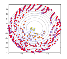
Fig. 1: Centrality-constrained embedding of the London tube

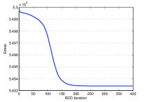
Fig. 2: MDS stress iterations

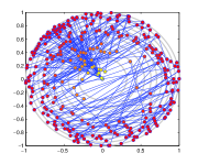
(a) $\lambda=0$

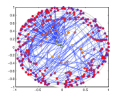
(b) $\lambda=1$

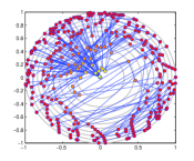
(c) $\lambda=100$

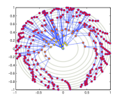
(d) $\lambda=10,000$

Fig. 3: Visualizing the London tube with a smoothing penalty

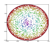
Fig. 4: Embedding of a large social network

5.2 Collaboration network of Arxiv General Relativity

In this experiment, a large social network is considered from the e-print arXiv repository covering scientific collaborations between authors on papers submitted to the “General Relativity and Quantum Cosmology” category (January $1993$ to April $2003$) [9]. The nodes represent authors and an edge exists between nodes $i$ and $j$ if authors $i$ and $j$ co-authored a paper. Although the network contains $5,242$ nodes, the embedding considered only its largest strongly connected component comprising $4,158$ nodes. The objective was to embed the network so that authors whose research is most related to the majority of the others are placed closer to the center.

This behavior is best captured by the closeness centrality that is defined as $c_{i}:=(\sum_{j\in\mathcal{V}}d_{ij})^{-1}$, where $d_{ij}$ is the geodesic distance (lowest sum of edge weights) between nodes $i$ and $j$; and captures the extent to which any node lies close to all other nodes [1, p. 88]. An informative mapping was obtained within $30$ outer iterations. For clarity and emphasis of the node positions, edges were not included in the visualization. Drawings of graphs as large as the autonomous systems within the Internet typically thin out most of the edges.

Figure 4 shows the embedding with color coding reflecting variations in centrality measure. The proposed approach based on first-order methods leads to a fast algorithm for visualizing such large networks.

6 CONCLUSIONS

In this work, MDS-based means of embedding graphs with certain structural constraints were proposed. In particular, an optimization problem was formulated under centrality constraints that are used to capture relative levels of importance between the nodes. A block coordinate descent solver with successive approximations was developed to deal with the non-convexity and non-smoothness of the constrained MDS stress minimization problem. In addition, a smoothness penalty term was incorporated to minimize the edge crossings in the resultant network visualizations. Tests on real-world networks were run and the results demonstrated that convergence is guaranteed, and large networks can be visualized relatively fast.

References

- [1] E. D. Kolaczyk, Statistical Analysis of Network Data: Methods and Models, Springer, New York, NY, USA, 2009.
- [2] I. Borg and P. J. F. Groenen, Modern Multidimensional Scaling: Theory and Applications, Springer, New York, NY, 2005.
- [3] U. Brandes and C. Pich, “More flexible radial layout,” J. of Graph Algorithms and Apps., vol. 15, pp. 157–173, Feb. 2011.
- [4] J. Alvarez-Hamelin, L. Dall’Asta, A. Barrat, and A. Vespignani, “Large scale networks fingerprinting and visualization using the k-core decomposition,” Advances in Neural Info. Proc. Sys., vol. 18, pp. 41–50, May 2006.
- [5] F. Fouss, A. Pirotte, J. M. Renders, and M. Saerens, “Random-walk computation of similarities between nodes of a graph with application to collaborative recommendation,” IEEE Trans. on Knowledge and Data Eng., vol. 19, pp. 355–369, March 2007.
- [6] A. Buja, D. F. Swayne, M. L. Littman, N. Dean, H. Hofmann, and L. Chen, “Data visualization with multidimensional scaling,” J. of Comp. and Graph. Stats., pp. 444–472, June 2008.
- [7] D. P. Bertsekas, Nonlinear programming, Athena Scientific, Belmont, MA, 1999.
- [8] M. Razaviyayn, M. Hong, and Z. Q. Luo, “A unified convergence analysis of block successive minimization methods for nonsmooth optimization,” arXiv preprint arXiv:1209.2385v1, Sept. 2012.
- [9] J. Leskovec, J. Kleinberg, and C. Faloutsos, “Graph evolution: Densification and shrinking diameters,” ACM Trans. on Knowledge Discovery from Data, vol. 1, article 2, March 2007.
- [10] L. C. Freeman, “A set of measures of centrality based on betweenness,” Sociometry, vol. 40, pp. 35–41, March 1977.