One-dimensional swimmers in viscous fluids:
dynamics, controllability, and existence
of optimal controls

Abstract.

In this paper we study a mathematical model of one-dimensional swimmers performing a planar motion while fully immersed in a viscous fluid. The swimmers are assumed to be of small size, and all inertial effects are neglected. Hydrodynamic interactions are treated in a simplified way, using the local drag approximation of resistive force theory. We prove existence and uniqueness of the solution of the equations of motion driven by shape changes of the swimmer. Moreover, we prove a controllability result showing that given any pair of initial and final states, there exists a history of shape changes such that the resulting motion takes the swimmer from the initial to the final state. We give a constructive proof, based on the composition of elementary maneuvers (straightening and its inverse, rotation, translation), each of which represents the solution of an interesting motion planning problem. Finally, we prove the existence of solutions for the optimal control problem of finding, among the histories of shape changes taking the swimmer from an initial to a final state, the one of minimal energetic cost.

1. Introduction

In this paper we study the self-propelled planar motions of a one-dimensional swimmer in an infinite viscous three-dimensional fluid. We are interested in the swimming strategies of small organisms that achieve self-propulsion by propagating bending waves along their slender bodies (such as, for instance, sperm cells and Caenorhabditis elegans). At these length scales, viscosity dominates over inertia: accordingly, we ignore all inertial effects in our analysis.

The study of the self-propulsion strategies of microscopic living organisms is attracting increasing attention, starting from seminal works by Taylor [26], Lighthill [21], Purcell [24], and Childress [8]. We refer the reader to the recent review [20] for a comprehensive list of references. Among the recent mathematical contributions we quote [19, 14, 25, 5, 2, 7, 4]. Many of these papers approach swimming problems within the framework of control theory, and this is exploited in [1, 3] for the numerical computation of energetically optimal strokes. While the connection between swimming and control theory is very natural, only recently has this point of view started to emerge and become widely appreciated, see [11] and the other chapters in the same volume.

When inertial forces are neglected, and external forces such as gravity are not present (neutrally buoyant swimmers), the equations of motion for a swimmer become the statements that the total viscous force and torque exerted by the surrounding fluid vanish. In order to take advantage of the simplifications deriving from the special one-dimensional geometry of our swimmers, we adopt here the local drag approximation of Resistive Force Theory, first introduced in [15], then also used in [23], and further discussed in [18]. It is a classical and popular theory widely spread among biological fluid dynamicists, which has recently been proved to be accurate and robust in the study of the motion of one-dimensional bodies in the length scales and regimes we are interested in, as it is shown, e.g., in [13]. According to resistive force theory, the external fluid exerts on the swimmer a viscous force per unit length which, at each point of the swimmer, is proportional to the local tangential and normal velocities at that point, through positive resistance coefficients denoted by $C_{\tau}$ and $C_{\nu}$, respectively.

For every $t$ in the time interval $[0,T]$, let $s\mapsto\chi(s,t)$ be the parametrization of the swimmer position with respect to an absolute external reference frame (lab frame), where $s\in[0,L]$ is the arc length parameter. It is possible to factorize this function as $\chi(s,t)=r(t)\circ\xi(s,t)$, where $r(t)$ is a time dependent rigid motion and $s\mapsto\xi(s,t)$ describes the shape of the swimmer at time $t$ with respect to a reference system moving with the swimmer (body frame).

We suppose that the shape function $\xi$ is given. The first problem we address in this paper is to determine the rigid motion $t\mapsto r(t)$ that results from a prescribed time history of shape changes $t\mapsto\xi(s,t)$. This is obtained by imposing that $\chi=r\circ\xi$ satisfies the equations of motion (the resultant of viscous forces and torques generated by the interaction between the swimmer and the fluid vanish for every $t$) and solving the resulting force and torque balance for $r$ in terms of the given $\xi$.

Our main result on this first problem is that, if $\xi$ satisfies suitable regularity conditions which are listed in the hypotheses of Theorem 3.3, then the rigid motion $r(t)$ can be determined as the unique solution of a system of ordinary differential equations in the independent variable $t$. Therefore, for every initial condition $r_{0}$, there exists a unique $r(t)$ such that the resulting function $\chi(s,t)=r(t)\circ\xi(s,t)$ satisfies the force and torque balance. In other words, Theorem 3.3 states that looking for a motion that satisfies the force and torque balance is equivalent to assigning the shape function and solving the equations of motion.

The second problem we address in this paper is that of controllability. Given a time interval $[0,T]$ and arbitrary initial and final states of the swimmer described by the arc length parametrizations $s\mapsto\chi_{\mathrm{in}}(s)$ and $s\mapsto\chi_{\mathrm{fin}}(s)$, can we find a self-propelled motion $\chi(s,t)$ in the lab frame such that $\chi(s,0)=\chi_{\mathrm{in}}(s)$ and $\chi(s,T)=\chi_{\mathrm{fin}}(s)$ ? By a self-propelled motion we mean one such that the equations of motion are satisfied which, in the case of self-propulsion, reduce to the vanishing of the total viscous force and torque. The answer is affirmative and is contained in Theorem 4.1. Our proof is constructive. Indeed, we exhibit an explicit procedure to transfer $\chi_{\mathrm{in}}$ onto $\chi_{\mathrm{fin}}$ based on the composition of elementary maneuvers: straightening of a curved configuration and the corresponding inverse maneuver (i.e., how to map a straight segment onto a given curved configuration), rotation of a straight segment around its barycenter, translation of a segment along its axis. Solving the motion planning problem for these elementary maneuvers is interesting in its own right, independently of the general controllability result, and this is done in Section 4.

More in detail, given two configurations $\chi_{\mathrm{in}}$ in $\chi_{\mathrm{fin}}$, we show how to straighten them in a segment-like configuration, say $\Sigma_{\mathrm{in}}$ and $\Sigma_{\mathrm{fin}}$, respectively, thanks to Theorem 3.3. Then we show how to transfer $\Sigma_{\mathrm{in}}$ into $\Sigma_{\mathrm{fin}}$, by explicitly constructing a way to make a rectilinear swimmer to translate (without rotating) along its axis, see Section 4.1, and a way to make it rotate (without translating) about its barycenter, see Section 4.2. These constructions use suitable bending wave forms that propagate along the body of the swimmer.

It is interesting to notice, and this will be clear in Section 4, that a very convenient way to describe such transformations is by using the angle that the tangent of the swimmer makes with the positive horizontal axis. This angle is given as a function of the time $t$ and of the arc length parameter $s$. This agrees with the traditional approach of prescribing the curvature function, since the latter can be recovered by differentiating the angle with respect to $s$ (see Remark 3.2). This classical approach is motivated by the fact that the swimmers we are interested in accomplish the shape changes required for force and torque balance by relative sliding of filaments along their “spine”, hence inducing local curvature changes.

The last problem we address is the existence of an energetically optimal swimming strategy. Here again we rely crucially on the simplification yielded by Resistive Force Theory since obtaining a similar result when the fluid-swimmer interaction is modeled by the Stokes equations is much more involved. In Theorem 5.1 we prove that, under suitable conditions, there exists a self-propelled motion $\chi(s,t)$ minimizing the power expended. The key hypothesis is a sort of non-interpenetration condition for the enlarged body obtained by thickening the curve describing the swimmer to a tube of constant thickness. This condition rules out self-intersections of the swimmer and yields an a-priori bound on its curvature.

2. Mathematical statement of the problem

In this section we describe the mathematical setting for studying the swimming problem by adapting to our specific case of a one-dimensional swimmer with a local fluid-swimmer interaction the framework introduced and described in [10, 22].

Throughout the paper we fix $L>0$ to be the length of the swimmer and $T>0$ so that $[0,T]$ is the time interval in which the motion occurs. We study planar motions in three dimensions, and therefore the position of each material point of the swimmer will be described by a function $\chi\colon[0,L]{\times}[0,T]\to\mathbb{R}^{2}$, where $s\in[0,L]$ is the arc length parameter; this request means that for every $t$ the map $s\mapsto\chi(s,t)$ is Lipschitz continuous from $[0,L]$ to $\mathbb{R}^{2}$ and $\left\lvert\chi^{\prime}(s,t)\right\rvert\equiv 1$, where $\chi^{\prime}:=\partial\chi/\partial s$. As for the derivative with respect to $t$, $\dot{\chi}:=\partial\chi/\partial t$ is intended in the distributional sense as the object that makes the following equality hold true

$$\int_{0}^{L}\!\!\int_{0}^{T}\dot{\chi}(s,t)\varphi(s,t)\,\mathrm{d}s\mathrm{d}t=-\int_{0}^{L}\!\!\int_{0}^{T}\chi(s,t)\frac{\partial\varphi(s,t)}{\partial t}\,\mathrm{d}s\mathrm{d}t\,,$$

for every $\varphi\in C^{\infty}_{\mathrm{c}}((0,L){\times}(0,T))$.

We now introduce the local expressions for the line densities $f(s,t)$ and $m(s,t)$ of viscous force and torque, as dictated by resistive force theory. Since $f(s,t)$ lies in the plane of the motion, $m(s,t)$ is orthogonal to it and is identified with a scalar. They are given by

$$\begin{split}f(s,t)=&\;-[C_{\tau}\,\dot{\chi}_{\tau}(s,t)\,\chi^{\prime}(s,t)+C_{\nu}\,\dot{\chi}_{\nu}(s,t)\,J\chi^{\prime}(s,t)]=-K_{\chi}(s,t)\dot{\chi}(s,t),\\ m(s,t)=&\;\left\langle f(s,t),J\chi(s,t)\right\rangle=-\left\langle C_{\tau}\,\dot{\chi}_{\tau}(s,t)\,\chi^{\prime}(s,t)+C_{\nu}\,\dot{\chi}_{\nu}(s,t)\,J\chi^{\prime}(s,t),J\chi(s,t)\right\rangle\\ =&-\left\langle K_{\chi}(s,t)\dot{\chi}(s,t),J\chi(s,t)\right\rangle.\end{split}$$ (2.1)

Here, $C_{\tau}$ and $C_{\nu}$ are positive constants, $\dot{\chi}_{\tau}$ and $\dot{\chi}_{\nu}$ are the tangential and normal components of the velocity $\dot{\chi}$, i.e., $\dot{\chi}_{\tau}(s,t)=\langle\dot{\chi}(s,t),$ $\chi^{\prime}(s,t)\rangle$ and $\dot{\chi}_{\nu}(s,t)=\left\langle\dot{\chi}(s,t),J\chi^{\prime}(s,t)\right\rangle$, while $J=\left[\begin{array}[]{cc}0&-1\\ 1&0\end{array}\right]$ is the counter-clockwise rotation matrix of angle $\pi/2$ and

$$K_{\chi}(s,t):=C_{\tau}\chi^{\prime}(s,t)\otimes\chi^{\prime}(s,t)+C_{\nu}(J\chi^{\prime}(s,t))\otimes(J\chi^{\prime}(s,t)),$$ (2.2)

where for any two vectors $a,b\in\mathbb{R}^{2}$ the matrix $a\otimes b$ is defined by $(a\otimes b)_{ij}=a_{i}b_{j}$ . The force and torque balance can be written as

$$0=F(t) \!\!\!\!:= \!\!\!\!\int_{0}^{L}f(s,t)\,\mathrm{d}s=-\int_{0}^{L}K_{\chi}(s,t)\dot{\chi}(s,t)\,\mathrm{d}s,$$ (2.3a)

$$0=M(t) \!\!\!\!:= \!\!\!\!\int_{0}^{L}m(s,t)\,\mathrm{d}s=-\int_{0}^{L}\left\langle K_{\chi}(s,t)\dot{\chi}(s,t),J\chi(s,t)\right\rangle\mathrm{d}s,$$ (2.3b)

for a.e. $t\in[0,T]$.

Remark 2.1.

An important remark on the structure of the viscous force and torque is in order, leading to a rate independence property. Let $\varphi$ be a $C^{1}$ strictly increasing function with $\varphi^{\prime}(t)>0$ for every $t\in[0,T]$. Then a rescaling in time by $\varphi$ has no consequences on the equations of motion. Indeed, we prove that if $\chi(s,t)$ satisfies the force and torque balance (2.3), then also $(\chi\circ\varphi)(s,t):=\chi(s,\varphi(t))$ does. Let us rewrite the force (2.3a) as $F_{\chi}(t)=-\int_{0}^{L}K_{\chi}(s,t)\dot{\chi}(s,t)\,\mathrm{d}s$. Then we have

$$\begin{split}F_{\chi\circ\varphi}(t)=&-\int_{0}^{L}K_{\chi\circ\varphi}(s,\varphi(t))\dot{\chi}(s,\varphi(t))\dot{\varphi}(t)\,\mathrm{d}s\\ =&-\dot{\varphi}(t)\int_{0}^{L}K_{\chi}(s,\varphi(t))\dot{\chi}(s,\varphi(t))\,\mathrm{d}s=\dot{\varphi}(t)F_{\chi}(\varphi(t))=0,\end{split}$$

since $F_{\chi}(\varphi(t))=0$ for a.e. $t\in[0,T]$. The same can be obtained for the torque $M_{\chi\circ\varphi}(t)$.

This rate independece character is at the root of the celebrated Scallop Theorem, see [24].

We conclude this section by introducing a function space $X$ containing our state functions, as well as the shape functions:

$$X:=\{\chi\colon[0,L]{\times}[0,T]\to\mathbb{R}^{2}:\chi\in L^{\infty}(0,T;H^{2}(0,L)),\,\dot{\chi}\in L^{2}(0,T;L^{2}(0,L))\},$$ (2.4)

endowed with the norm

$$\left\lVert\chi\right\rVert_{X}:=\operatorname*{ess\,sup}_{0\leqslant t\leqslant T}\left\lVert\chi(\cdot,t)\right\rVert_{H^{2}(0,L)}+\left(\int_{0}^{T}\lVert\dot{\chi}(\cdot,t)\rVert_{L^{2}(0,L)}^{2}\,\mathrm{d}t\right)^{1/2},$$ (2.5)

which makes it a Banach space. It follows from the definition that

$$X\subset H^{1}(0,T;L^{2}(0,L))\text{ with continuous embedding}.$$ (2.6)

Since every function $\chi$ in $H^{1}(0,T;L^{2}(0,L))$ can be modified on a negligible subset of $[0,T]$ so that $t\mapsto\chi(\cdot,t)$ is strongly continuous from $[0,T]$ into $L^{2}(0,L)$, we shall always refer to this modified function when we consider the properties of $\chi(\cdot,t)$ for some $t\in[0,T]$. With this convention we have

$$X\subset C^{0}([0,T];L^{2}(0,L))\text{ with continuous embedding}.$$ (2.7)

The following proposition shows the main properties of the space $X$.

Proposition 2.2.

Let $\chi\in X$. Then for every $t\in[0,T]$ we have $\chi(\cdot,t)\in H^{2}(0,L)$ and

$$\left\lVert\chi(\cdot,t)\right\rVert_{H^{2}(0,L)}\leqslant\left\lVert\chi\right\rVert_{X}.$$ (2.8)

Moreover, the function $t\mapsto\chi(\cdot,t)$ is continuous with respect to the weak topology of $H^{2}(0,L)$. Finally,

$$\chi\in C^{0}([0,T];C^{1}([0,L])),$$ (2.9)

$$\left\lVert\chi\right\rVert_{C^{0}([0,T];C^{1}([0,L]))}\leqslant C\left\lVert\chi\right\rVert_{X}\,,$$ (2.10)

where the constant $C$ is independent of $\chi$.

Proof.

To prove the first claim, let us fix $t\in[0,T]$ and let $N$ be a zero measure set up to which the essential supremum in (2.5) is actually a supremum. Consider a sequence $t_{n}\notin N$ converging to $t$, so that $\left\lVert\chi(\cdot,t_{n})\right\rVert_{H^{2}(0,L)}\leqslant\left\lVert\chi\right\rVert_{X}$ . Since $\chi(\cdot,t_{n})\to\chi(\cdot,t)$ in $L^{2}([0,L])$ by (2.7), we have that $\chi(\cdot,t)\in H^{2}(0,L)$. Moreover, since the $H^{2}$ norm is lower-semicontinuous, we have also

$$\left\lVert\chi(\cdot,t)\right\rVert_{H^{2}(0,L)}\leqslant\liminf_{n\to+\infty}\left\lVert\chi(\cdot,t_{n})\right\rVert_{H^{2}(0,L)}\leqslant\left\lVert\chi\right\rVert_{X},$$

which proves (2.8). Thanks to this inequality, the strong continuity of the function $t\mapsto\chi(\cdot,t)$ in $L^{2}([0,L])$ implies the weak continuity in $H^{2}(0,L)$. Then the compact embedding of $H^{2}(0,L)$ into $C^{1}([0,L])$ implies that the function $t\mapsto\chi(\cdot,t)$ is continuous with respect to the strong topology of $C^{1}([0,L])$, which gives (2.9). Finally, (2.10) follows from (2.8) and from the continuous embedding of $H^{2}(0,L)$ into $C^{1}([0,L])$. ∎

Note that, by (2.9), for every $\chi\in X$ we have

$$\chi,\,\chi^{\prime}\in C^{0}([0,L]{\times}[0,T]).$$ (2.11)

We are interested only in functions $\chi\in X$ such that $s\mapsto\chi(s,t)$ is the arc length parametrization of a curve; this leads to the following definition

$$X_{1}:=\{\chi\in X:\left\lvert\chi^{\prime}\right\rvert=1\text{ in $[0,L]{\times}[0,T]$}\}.$$ (2.12)

3. Equations of motion

In this section we derive the equations of motion for the swimmer. It is convenient to factorize the function $\chi\in X_{1}$ as the composition of a time dependent rigid motion $r$, which represents the change of location, with a function $\xi\in X_{1}$, which represents the change of shape. We write

$$\chi(s,t)=x(t)+R(t)\xi(s,t),$$ (3.1)

where $x(t)\in\mathbb{R}^{2}$ is the translation vector and $R(t)\in\mathbb{R}^{2{\times}2}$ is the rotation corresponding to the rigid motion $r(t)$.

If we assume that $\int_{0}^{L}\xi(s,t)\,\mathrm{d}s=0$ for every $t\in[0.T]$, then $x(t)$ coincides with the barycenter of the curve $\chi(\cdot,t)$, which describes the swimmer at time $t$ with respect to the absolute reference system, while the function $\xi(\cdot,t)$ will be regarded as the deformation seen by an observer moving with barycenter of the swimmer.

Proposition 3.1.

Let $\xi\in X_{1}$ and let $x\colon[0,T]\to\mathbb{R}^{2}$ and $R\colon[0,T]\to\mathbb{R}^{2{\times}2}$ be functions such that $R(t)$ is a rotation for every $t\in[0,T]$. Then the following properties are equivalent:

• the function $\chi$ defined by (3.1) belongs to $X_{1}$ ;

• the functions $x$ and $R$ belong to $H^{1}(0,T)$.

Proof.

(i)$\Rightarrow$(ii). For every $t\in[0,T]$ we define

$$\overline{\xi}(t):=\frac{1}{L}\int_{0}^{L}\xi(s,t)\,\mathrm{d}s\qquad\text{and}\qquad\overline{\chi}(t):=\frac{1}{L}\int_{0}^{L}\chi(s,t)\,\mathrm{d}s.$$

Since $\xi,\,\chi\in X_{1}\subset H^{1}(0,T;L^{2}(0,L))$ we have that $\overline{\xi},\,\overline{\chi}\in H^{1}(0,T)$. By averaging (3.1) with respect to $s$ we obtain

$$\overline{\chi}(t)=x(t)+R(t)\overline{\xi}(t).$$ (3.2)

Subtracting this equation from (3.1) we obtain

$$\chi(s,t)-\overline{\chi}(t)=R(t)\big{(}\xi(s,t)-\overline{\xi}(t)\big{)}.$$ (3.3)

Let us fix $t_{0}\in[0,T]$. Since $|\xi^{\prime}(s,t_{0})|=1$ for every $s\in[0,L]$, there exists $s_{0}\in[0,L]$ such that $\xi(s_{0},t_{0})-\overline{\xi}(t_{0})\neq 0$. By the continuity of $\xi$ there exist $\varepsilon>0$, an open neighborhood $U$ of $s_{0}\in[0,L]$, and an open neighborhood $V$ of $t_{0}$ in $[0,T]$ such that $\left\lvert\chi(s,t)-\overline{\chi}(t)\right\rvert=\left\lvert\xi(s,t)-\overline{\xi}(t)\right\rvert\geqslant\varepsilon$ for every $s\in U$ and every $t\in V$, where the equality follows from (3.3). Let $\chi^{*}(s,t):=\big{(}\chi(s,t)-\overline{\chi}(t)\big{)}/\left\lvert\chi(s,t)-\overline{\chi}(t)\right\rvert$ and $\xi^{*}(s,t):=\big{(}\xi(s,t)-\overline{\xi}(t)\big{)}/\left\lvert\xi(s,t)-\overline{\xi}(t)\right\rvert$. By (3.3) we have

$$\chi^{*}(t,s)=R(t)\xi^{*}(t,s)$$

for every $s\in U$ and every $t\in V$. By elementary Linear Algebra we have

$$R(t)=\left[\begin{array}[]{cc}\left\langle\chi^{*}(s,t),\xi^{*}(s,t)\right\rangle&-\left\langle\chi^{*}(s,t),J\xi^{*}(s,t)\right\rangle\\ \left\langle\chi^{*}(s,t),J\xi^{*}(s,t)\right\rangle&\left\langle\chi^{*}(s,t),\xi^{*}(s,t)\right\rangle\end{array}\right].$$ (3.4)

By (2.6) and (2.9) the functions $\chi^{*}$ and $\xi^{*}$ belong to $H^{1}(V;L^{2}(U))\cap C^{0}(\overline{V};C^{1}(U))$, so that the entries of the matrix in (3.4) belong to $H^{1}(V;L^{2}(U))$. Since the matrix does not depend on $s$, we obtain $R\in H^{1}(V)$. The conclusion $R\in H^{1}(0,T)$ follows now from a covering argument.

Since $\overline{\chi}$, $R$, and $\overline{\xi}$ belong to $H^{1}(0,T)$, we deduce from (3.2) that $x\in H^{1}(0,T)$.

(ii)$\Rightarrow$(i). This implication follows easily from (2.4) and (3.1). ∎

Remark 3.2.

The purpose of the function $\xi(\cdot,t)$ is to describe the shape of the swimmer as a function of time. For each $t$ we can choose the most convenient reference system. Of course, different choices are compensated by different rigid motions in (3.1).

In many cases it is convenient to describe the shape of the swimmer by means of the (oriented) curvature $\kappa(s,t)$ of the curve $\xi(\cdot,t)$ at $s$. This is because both in living organisms and in technological devices shape changes are usually obtained by controlling the mutual distance of several pairs of points. Prescribing the curvature can be interpreted as the infinitesimal version of this control, whose description is easier from the mathematical point of view.

If $\chi\in X_{1}$ and $\xi\in X_{1}$ are linked by (3.1), then clearly their curvatures are the same. Given $\xi\in X_{1}$, let $\vartheta(s,t)$ be the oriented angle between the $x_{1}$-axis and the oriented tangent to the curve $\xi(\cdot,t)$ at $s$. It is well known that $\kappa(s,t)=\left\langle\xi^{\prime\prime}(s,t),J\xi^{\prime}(s,t)\right\rangle=\vartheta^{\prime}(s,t)$, so we can easily get $\kappa$ from $\xi$ by differentiation and $\vartheta$ from $\kappa$ by integration. In particular, if we assume $\xi^{\prime}(0,t)=e_{1}$, we have $\vartheta(0,t)=0$, hence

$$\vartheta(s,t)=\int_{0}^{s}\kappa(\sigma,t)\,\mathrm{d}\sigma.$$

Then the definition of $\vartheta(s,t)$ gives that $\xi^{\prime}(s,t)=(\cos\vartheta(s,t),\sin\vartheta(s,t))$, so that, if $\xi(0,t)=0$, we have

$$\xi(s,t)=\int_{0}^{s}(\cos\vartheta(\sigma,t),\sin\vartheta(\sigma,t))\,\mathrm{d}\sigma.$$

This shows that the descriptions of the shape given by $\xi(s,t)$ and $\kappa(s,t)$ are equivalent.

By the change of reference (3.1), it is possible to rephrase the force and torque balance (2.3) and eventually obtain ordinary differential equations governing the time evolution of $x$ and $R$. Those will be the equations of motion of the swimmer. We can write

$$R(t)=\left[\begin{array}[]{cc}\cos\theta(t)&-\sin\theta(t)\\ \sin\theta(t)&\cos\theta(t)\end{array}\right],$$

where $\theta(t)$ is the angle of rotation. We assume that $\xi$ and $\chi$ belong to $X_{1}$. Thanks to Proposition 3.1, we can differentiate (3.1) with respect to time. Plugging all the terms in (2.3) and noticing that $K_{\chi}(s,t)=R(t)K_{\xi}(s,t)R^{\top}(t)$, we obtain

$$\!\!\!\!\left(\begin{array}[]{c}F(t)\\ M_{x}(t)\end{array}\right)\!=\!\left[\begin{array}[]{cc}R(t)&0\\ 0&1\end{array}\right]\left\{-\left[\begin{array}[]{cc}A(t)&b(t)\\ b^{\top}(t)&c(t)\end{array}\right]\!\left[\begin{array}[]{cc}R^{\top}(t)&0\\ 0&1\end{array}\right]\!\left(\begin{array}[]{c}\dot{x}(t)\\ \dot{\theta}(t)\end{array}\right)+\left(\begin{array}[]{c}F^{\mathrm{sh}}(t)\\ M^{\mathrm{sh}}(t)\end{array}\right)\right\},$$ (3.5)

where $M_{x}(t):=M(t)-\left\langle F(t),Jx(t)\right\rangle$ and $\mathcal{R}(t)=\left[\begin{array}[]{cc}A(t)&b(t)\\ b^{\top}(t)&c(t)\end{array}\right]$ is the grand resistance matrix of [17], whose entries are given by

$$A(t):=\!\int_{0}^{L}\!K_{\xi}(s,t)\,\mathrm{d}s,\quad b(t):=\!\int_{0}^{L}\!K_{\xi}(s,t)J\xi(s,t)\,\mathrm{d}s,$$ (3.6a)

$$c(t):=\!\int_{0}^{L}\!\left\langle J\xi(s,t),K_{\xi}(s,t)J\xi(s,t)\right\rangle\,\mathrm{d}s.$$ (3.6b)

It is easy to see that the functions $A$, $b$, and $c$ are ultimately determined by the shape function $\xi$ alone. The terms

$$F^{\mathrm{sh}}(t):=-\int_{0}^{L}K_{\xi}(s,t)\dot{\xi}(s,t)\,\mathrm{d}s,\qquad M^{\mathrm{sh}}(t):=-\int_{0}^{L}\langle J\xi(s,t),K_{\xi}(s,t)\dot{\xi}(s,t)\rangle\,\mathrm{d}s,$$ (3.7)

are the contributions to the force and torque due to the shape deformation of the swimmer, and they depend linearly on the time derivative $\dot{\xi}$.

Enforcing the force and torque balance (2.3) is equivalent to setting (3.5) equal to zero and solving for $\dot{x}$ and $\dot{\theta}$, which eventually leads to the equations

$$\left\{\begin{array}[]{rl}\dot{x}(t)&\!\!\!\!=R(t)v(t),\\[2.0pt] \dot{\theta}(t)&\!\!\!\!=\omega(t),\end{array}\right.$$ (3.8)

where

$$v(t):=\bar{A}(t)F^{\mathrm{sh}}(t)+\bar{b}(t)M^{\mathrm{sh}}(t),\qquad\omega(t):=\bar{b}^{\top}(t)F^{\mathrm{sh}}(t)+\bar{c}(t)M^{\mathrm{sh}}(t),$$ (3.9)

and $\bar{A}(t)$, $\bar{b}(t)$, and $\bar{c}(t)$ are the block elements of the inverse matrix $\mathcal{R}^{-1}(t)$. The structure of this system of ordinary differential equations is the same as that previously obtained in [3, 10]. The following result, analogous to [10, Theorem 6.4], holds

Theorem 3.3.

Let $\xi\in X_{1}\,$, $x_{0}\in\mathbb{R}^{2}$, and $\theta_{0}\in\mathbb{R}$. Then the equations of motion (3.8), with initial conditions $x(0)=x_{0}$ and $\theta(0)=\theta_{0}$, have a unique absolutely continuous solution $t\mapsto(x(t),\theta(t))$ defined in $[0,T]$ with values in $\mathbb{R}^{2}{\times}\mathbb{R}$. This solution actually belongs to $H^{1}(0,T)$. In other words, there exists a unique rigid motion $t\mapsto r(t)$, such that the deformation function defined by (3.1) belongs to $X_{1}$, satisfies the equations of motion (2.3), and the initial conditions $x(0)=x_{0}$ and $R(0)=R_{\theta_{0}}\,$, the rotation of angle $\theta_{0}$.

Proof.

The result easily follows from the classical theory of ordinary differential equations, see, e.g., [16]. Indeed, the coefficients $\bar{b}^{\top}$ and $\bar{c}$ are continuous function of $t$, since they come from the inversion of the grand resistance matrix $\mathcal{R}$, whose entries are continuous in $t$. On the contrary, $F^{\mathrm{sh}}$ and $M^{\mathrm{sh}}$ are only $L^{2}$ functions of time. This is enough to integrate the second equation in (3.8). By plugging the solution for $\theta$ into the first equation and by an analogous argument on the coefficients $\bar{A}$ and $\bar{b}$, also the equation for $x$ has a unique solution with prescribed initial data.

The last statement follows esily from Proposition 3.1. ∎

Some notes on the matrix $K$ and on the coefficients $C_{\tau}$ and $C_{\nu}$ are in order. First, we assume that

$$0<C_{\tau}<C_{\nu}\,,$$ (3.10)

secondly, we notice that the matrix $K_{\chi}$ (and therefore $K_{\xi}$) is symmetric and positive definite, and defines a scalar product in the space $X_{1}$ . Indeed, by introducing the power expended during the motion

$$\begin{split}\mathcal{P}(\chi):=&\int_{0}^{T}\!\!\int_{0}^{L}\left\langle-f(s,t),\dot{\chi}(s,t)\right\rangle\,\mathrm{d}s\mathrm{d}t=\int_{0}^{T}\!\!\int_{0}^{L}\left\langle K_{\chi}(s,t)\dot{\chi}(s,t),\dot{\chi}(s,t)\right\rangle\,\mathrm{d}s\mathrm{d}t\\ =&\int_{0}^{T}\!\!\int_{0}^{L}[C_{\tau}\dot{\chi}^{2}_{\tau}(s,t)+C_{\nu}\dot{\chi}^{2}_{\nu}(s,t)]\,\mathrm{d}s\mathrm{d}t,\end{split}$$ (3.11)

we find that

$$C_{\tau}\left\lVert\dot{\chi}\right\rVert_{L^{2}(0,T;L^{2}(0,L))}^{2}\leqslant\mathcal{P}(\chi)\leqslant C_{\nu}\left\lVert\dot{\chi}\right\rVert_{L^{2}(0,T;L^{2}(0,L))}^{2}\,.$$

Moreover, it follows from (2.2) and (2.11) that the matrices $K_{\xi}$ and $K_{\chi}$ are continuous in $(s,t)$.

Finally, the strict inequality assumption $C_{\tau}<C_{\nu}$ cannot be weakened. Indeed, if we had $C_{\tau}=C_{\nu}$ , then $K_{\chi}(s,t)$ would be a multiple of the identity matrix and therefore, from (2.3a), we would have

$$0=F(t)=-C_{\tau}\int_{0}^{L}\dot{\chi}(s,t)\,\mathrm{d}s=-C_{\tau}\frac{\mathrm{d}}{\mathrm{d}t}\left(\int_{0}^{L}\chi(s,t)\,\mathrm{d}s\right),$$

which is expressing that the barycenter does not move as time evolves.

3.1. The shape function

We introduce now an important assumption on the shape function $\xi$, called two disks condition, which rules out self-intersections of the swimmer. This hypothesis will be crucial in the proof of the existence of an optimal swimming strategy. The idea underlying this condition is that two distinct points of the swimmer cannot become too close to each other during the motion.

Definition 3.4.

We say that $\xi\in H^{2}(0,L;\mathbb{R}^{2})$ with $\left\lvert\xi^{\prime}(s)\right\rvert=1$ for every $s\in[0,L]$ satisfies the two disks condition with radius $\rho>0$ if the following conditions are satisfied (see Fig. 1):

• for every $s\in[0,L]$ there exist open disks $B^{1}(s),B^{2}(s)$ of radius $\rho>0$ such that $B^{1}(s)\cap B^{2}(s)=\mathchar 31\relax$, $\xi(s)\in\overline{B}{}^{1}(s)\cap\overline{B}{}^{2}(s)$, and $\xi(\sigma)\notin B^{1}(s)\cup B^{2}(s)$ for every $\sigma\in[0,L]$;

• there exist open half disks $B^{-},B^{+}$ of radius $2\rho$ centered at $\xi(0)$ and $\xi(L)$, respectively, with diameters normal to $\xi^{\prime}(0)$ and $\xi^{\prime}(L)$, respectively, such that $\xi(\sigma)\notin B^{-}\cup B^{+}$ for every $\sigma\in[0,L]$.

Since $\xi$ is of class $C^{1}$ and $\left\lvert\xi^{\prime}(s)\right\rvert=1$, the disks considered in condition (a) are uniquely determined by $\xi(s)$ and $\xi^{\prime}(s)$. Indeed, they are the disks with centers $\xi(s)\pm\rho J\xi^{\prime}(s)$ and radius $\rho$. In the sequel we will always assume that

$$B^{1}(s)=B_{\rho}(\xi(s)+\rho J\xi^{\prime}(s)),\qquad B^{2}(s)=B_{\rho}(\xi(s)-\rho J\xi^{\prime}(s)).$$ (3.12)

The following proposition proves an important consequence of the two disks condition.

Proposition 3.5.

Let $\xi\in H^{2}(0,L;\mathbb{R}^{2})$ with $\left\lvert\xi^{\prime}(s)\right\rvert=1$ for every $s\in[0,L]$. Assume that $\xi$ satisfies the two disks condition for some radius $\rho>0$. Then $\xi$ is injective on $[0,L]$.

Proof.

Assume by contradiction that there exist $s_{1}<s_{2}$ such that $\xi(s_{1})=\xi(s_{2})$. It is easy to see that the two disks condition implies that $\xi^{\prime}(s_{1})=\pm\xi^{\prime}(s_{2})$. Assume that $\xi^{\prime}(s_{1})=\xi^{\prime}(s_{2})$ , the other case being analogous. Since these derivatives have norm 1, by changing the coordinate system we may assume that $\xi^{\prime}(s_{1})=\xi^{\prime}(s_{2})=e_{1}$ , the first vector of the canonical basis. We denote the coordinates of $\xi$ by $\xi_{1}$ and $\xi_{2}$ and we set $\alpha:=\xi_{1}(s_{1})=\xi_{1}(s_{2})$ and $\beta:=\xi_{2}(s_{1})=\xi_{2}(s_{2})$. By the Local Inversion Theorem, there exist $\varepsilon>0$, $\delta>0$, and a $C^{1}$ function $g:(\alpha-\varepsilon,\alpha+\varepsilon)\to\mathbb{R}$ such that for every $s\in(s_{1}-\delta,s_{1}+\delta)\cap[0,L]$ we have $\left\lvert\xi_{1}(s)-\alpha\right\rvert<\varepsilon$ and $\xi_{2}(s)=g(\xi_{1}(s))$. Let

$$E^{1}:=\bigcup_{\left\lvert s-s_{1}\right\rvert<\delta}B^{1}(s),\qquad E^{2}:=\bigcup_{\left\lvert s-s_{1}\right\rvert<\delta}B^{2}(s).$$

By (3.12) it is easy to see that there exists an open rectangle $R$ centered at $(\alpha,\beta)$ such that $E^{1}\cap R=\{(a,b)\in R:b>g(a)\}$ and $E^{2}\cap R=\{(a,b)\in R:b<g(a)\}$. By condition (a) of Definition 3.4 $\xi(s)\in\{(a,b)\in R:b=g(a)\}$ for every $s\in[0,L]$ such that $\xi(s,t)\in R$. Therefore, $s\mapsto\xi(s)$ is locally an arc length parametrization of the graph of $g$. Since $\xi(s_{1})=\xi(s_{2})=(\alpha,\beta)$ and $\xi^{\prime}(s_{1})=\xi^{\prime}(s_{2})=e_{1}$ , there exists $\eta>0$ such that $\xi(s_{1}+s)=\xi(s_{2}+s)$ for $\left\lvert s\right\rvert<\eta$, provided $0\leqslant s_{1}+s<s_{2}+s\leqslant L$. This implies that $\xi(\sigma-(s_{2}-s_{1}))=\xi(\sigma)$ for every $\sigma$ in a neighborhood of $s_{2}$ in $[0,L]$ such that $\sigma-(s_{2}-s_{1})\in[0,L]$. By taking the supremum $\sigma_{0}$ over $\sigma$, we obtain that $\xi(\sigma_{0})=\xi(L)$ for $\sigma_{0}:=L-(s_{2}-s_{1})\in[0,L)$. If $\sigma_{0}>0$, we deduce also that $\xi^{\prime}(\sigma_{0})=\xi^{\prime}(L)$. The same equality holds when $\sigma_{0}=0$, because in this case $\sigma_{0}=s_{1}=0$ and $s_{2}=L$, so that the equality follows from the assumption $\xi^{\prime}(s_{1})=\xi^{\prime}(s_{2})$.

Let $B^{+}$ be the half disk considered in condition (b) of Definition 3.4. By the previous equalities, $\xi(\sigma_{0})$ is the center of $B^{+}$ and $\xi^{\prime}(\sigma_{0})$ points towards the interior. It follows that $\xi(\sigma)\in B^{+}$ for some $\sigma>\sigma_{0}$ , and this contradicts condition (b). ∎

Figure 1. Two disks condition: $B^{1}(s)$ and $B^{2}(s)$ are the open disks of radius $\rho$, $B^{-}$ and $B^{+}$ are the open half disks of radius $2\rho$. The dashed line represents the image of the map $h$ defined in (3.13).

Given $\rho>0$ we introduce $C_{L,\rho}:=([0,L]{\times}\{0\})+B_{\rho}(0)$, the cigar-like set obtained by enlarging $[0,L]{\times}\{0\}$. Define now a map $h\colon[0,L]{\times}(-\rho,\rho)\to\mathbb{R}^{2}$ by

$$h(s,y):=\xi(s)+yJ\xi^{\prime}(s).$$ (3.13)

This map is extended to a continuous map $h\colon C_{L,\rho}\to\mathbb{R}^{2}$ by defining it as an isometry mapping $C_{L,\rho}\cap\{s<0\}$ into the half disk $\frac{1}{2}B^{-}$ homothetic to the half disk $B^{-}$ considered in condition (b) of Definition 3.4, with the same center and half the radius; the definition in $C_{L,\rho}\cap\{s>L\}$ is similar and uses the half disk $\frac{1}{2}B^{+}$ (see Fig. 1). The following proposition improves Proposition 3.5 and provides an equivalent formulation of Definition 3.4.

Proposition 3.6.

Let $\xi\in H^{2}(0,L;\mathbb{R}^{2})$ with $\left\lvert\xi^{\prime}(s)\right\rvert=1$ for every $s\in[0,L]$, and let $\rho>0$. The map $h$ is injective if and only if $\xi$ satisfies the two disks condition with radius $\rho$.

Proof.

Let us assume that the two disks condition holds and let us consider two points $(s_{1},y_{1})\neq(s_{2},y_{2})$ in $C_{L,\rho}$ . If $0\leqslant s_{1}=s_{2}\leqslant L$, then it must be $\left\lvert y_{1}-y_{2}\right\rvert>0$, and therefore $|h(s_{1},y_{1})-h(s_{1},y_{2})|=\left\lvert y_{1}-y_{2}\right\rvert>0$. If $-\rho<s_{1}=s_{2}<0$, then $h(s_{1},y_{1})\neq h(s_{1},y_{2})$ since $h$ is an isometry on $C_{L,\rho}\cap\{s<0\}$. The same conclusion holds if $L<s_{1}=s_{2}<L+\rho$.

Assume now that $0\leqslant s_{1}<s_{2}\leqslant L$. If $y_{1}=y_{2}=0$, then $h(s_{1},y_{1})=\xi(s_{1})\neq\xi(s_{2})=h(s_{2},y_{2})$, where the inequality follows from the fact that the curve $\xi(\cdot,t)$ is injective by Proposition 3.5. If $y_{1}\neq 0=y_{2}$ , then $h(s_{1},y_{1})$ belongs to one of the disks $B^{1}(s_{1})\,,B^{2}(s_{1})$ introduced in condition (a) of Definition 3.4. It follows that $h(s_{2},y_{2})=\xi(s_{2})\notin B^{1}(s_{1})\cup B^{2}(s_{1})$ , hence $h(s_{1},y_{1})\neq h(s_{2},y_{2})$. The same conclusion holds if $y_{1}=0\neq y_{2}$ .

Let us consider now the case $0\leqslant s_{1}<s_{2}\leqslant L$ and $y_{1}\neq 0\neq y_{2}$ . Define $S_{i}:=\{\xi(s_{i})+yJ\xi^{\prime}(s_{i}):0<(\operatorname{sign}y_{i})y<\rho\}$ for $i=1,2$. Let us prove that

$$S_{1}\cap S_{2}=\mathchar 31\relax.$$ (3.14)

Let $p_{i}:=\xi(s_{i})$ and let $D_{i}$ be the open disk with center $c_{i}:=\xi(s_{i})+\operatorname{sign}(y_{i})\rho J\xi^{\prime}(s_{i})$ and radius $\rho$. Note that $c_{i}$ and $p_{i}$ are the endpoints of $S_{i}$ and that $p_{1}\neq p_{2}$ since the map $s\mapsto\xi(s)$ is injective by Proposition 3.5. If $c_{1}=c_{2}$ , then $S_{1}\cap S_{2}=\mathchar 31\relax$ because $S_{1},S_{2}$ are radii of the same circle with different endpoints.

We consider now the case $c_{1}\neq c_{2}$ . Since $D_{1}$ is one of the disks $B^{1}(s_{1}),B^{2}(s_{1})$, by condition (a) of Definition 3.4, we have that $p_{1}=\xi(s_{1})\in\partial D_{1}$ and $p_{2}=\xi(s_{2})\notin D_{1}$ . Similarly, we prove that $p_{2}\in\partial D_{2}$ and $p_{1}\notin D_{2}$ . Therefore, $p_{1}\in\partial D_{1}\setminus D_{2}$ and $p_{2}\in\partial D_{2}\setminus D_{1}$ .

Assume by contradiction that $S_{1}$ and $S_{2}$ meet at some point $p$, which must belong to $D_{1}\cap D_{2}$ . Let $z$ be the intersection between $\partial D_{2}$ and the half-line stemming from $c_{2}$ and containing $c_{1}$; under our assumptions, we have $z\in D_{1}$ . Since $p\in D_{1}\cap D_{2}$ and $p_{1}\in\partial D_{1}\setminus D_{2}$ , there exists a unique point $q\in\partial D_{2}\cap D_{1}$ on the segment joining $p$ and $p_{1}$ . Now, the half-line through $p$ stemming from $c_{2}$ meets $\partial D_{2}$ on the smallest arc $\Gamma$ with endpoints $q$ and $z$. Since $q,z\in D_{1}$ and the disks have the same radius, we have $\Gamma\subset D_{1}$ (see Fig. 2). The previous argument shows that $p_{2}\in\Gamma$, which contradicts the condition $p_{2}\in\partial D_{2}\setminus D_{1}$ . This concludes the proof of the equality $S_{1}\cap S_{2}=\mathchar 31\relax$ in the case $0\leqslant s_{1}<s_{2}\leqslant L$ and $y_{1}\neq 0\neq y_{2}$ , and implies that $h(s_{1},y_{1})\neq h(s_{2},y_{2})$.

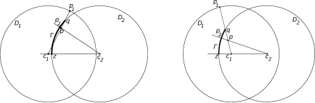
Figure 2. Injectivity for $0\leqslant s_{1}<s_{2}\leqslant L$ and $y_{1}\neq 0\neq y_{2}$ in the case $c_{1}\neq c_{2}$ : Two possible situations contradicting (3.14).

We consider now the case $0\leqslant s_{1}<L<s_{2}<L+\rho$. Assume by contradiction that $h(s_{1},y_{1})=h(s_{2},y_{2})=:p$. Observe that $p\in\frac{1}{2}B^{+}$. Denote $p_{1}:=\xi(s_{1})$ and $S:=\{\xi(L)+yJ\xi^{\prime}(L):-\rho<y<\rho\}$. By (3.14) for $s_{1}$ and $L$ the segment with endpoints $p,p_{1}$ does not intersect $S$. On the other hand $\left\lvert p-p_{1}\right\rvert=\left\lvert y_{1}\right\rvert<\rho$. By elementary geometric arguments we find that the set $Q$ of points which can be connected to a point of $\frac{1}{2}B^{+}$ by a segment disjoint from $S$ and of length less than $\rho$ is contained in the union $B^{+}\cup B^{1}(L)\cup B^{2}(L)$ (See Fig. 3). Therefore $p_{1}=\xi(s_{1})\in Q$ and this violates either condition (a) or condition (b) in Definition 3.4.

In the case $s_{1}=L<s_{2}<L+\rho$, we have $h(s_{1},y_{1})\in\partial(\frac{1}{2}B^{+})$, while $h(s_{2},y_{2})\in\frac{1}{2}B^{+}$, so that $h(s_{1},y_{1})\neq h(s_{2},y_{2})$. The cases $-\rho<s_{1}<0<s_{2}\leqslant L$ and $-\rho<s_{1}<0=s_{2}$ are analogous.

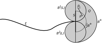
Figure 3. Injectivity for $0\leqslant s_{1}\leqslant L<s_{2}<L+\rho$. The shaded region represents the set $Q$; the thick segment is the set $S$.

The last case to consider is when $-\rho<s_{1}<0$ and $L<s_{2}<L+\rho$. Assume, by contradiction, that $h(s_{1},y_{1})=h(s_{2},y_{2})$. Since the radius of curvature of $\xi$ is always less than $\rho$, one can prove (see Lemma 3.7 below and Fig. 4) that

$$D^{-}\subset B^{-}\cup\bigcup_{0\leq s\leq\frac{\pi}{2}\rho}\big{(}B^{1}(s)\cup\{\xi(s)\}\cup B^{2}(s)\big{)}\,,$$ (3.15)

where $D^{-}:=\{x\in\mathbb{R}^{2}:d(x,\frac{1}{2}B^{-}){<\,}\rho\}$ and $B^{1}(s),\,B^{2}(s)$ are the open disks defined in (3.12).

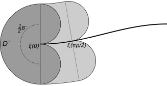
Figure 4. The region $D^{-}$ of (3.15).

Since $h(s_{1},y_{1})\in\frac{1}{2}B^{-}$, $h(s_{1},y_{1})=h(s_{2},y_{2})$, and $|h(s_{2},y_{2})-\xi(L)|<\rho$, we deduce that $\xi(L)\in D^{-}$. By (3.15) either $\xi(L)\in B^{-}$ or there exists $s\in[0,\frac{\pi}{2}]$ such that $\xi(L)\in B^{1}(s)\cup\{\xi(s)\}\cup B^{2}(s)$. This contradicts Definition 3.4 or Proposition 3.5, and concludes the proof in this case.

Let us now assume that $h$ is injective, and consider $s\in[0,L]$. Let $B^{1}(s),\,B^{2}(s)$ the open disks defined in (3.12). It is clear that $B^{1}(s)\cap B^{2}(s)=\mathchar 31\relax$ and $\overline{B}{}^{1}(s)\cap\overline{B}{}^{2}(s)=\{\xi(s)\}$. Denote by $N(s):=\{\xi(s)+yJ\xi^{\prime}(s),y\in\mathbb{R}\}$ the normal line through the point $\xi(s)$, and let $\widetilde{\xi}(s):=\xi(s)+\frac{1}{\kappa(s)}J\xi^{\prime}(s)$ be the evolute of $\xi$, i.e., the curve that contains the centers of the osculating circles to $\xi$. Since $\xi$ is a curve of class $H^{2}$, the curvature is well defined almost everywhere; let $s_{1}\in(0,L)$ be a point at which the curvature $\kappa(s_{1})$ is defined, and let $s_{2}\in(0,L)$ be another point. By the injectivity of $h$, the normal lines $N(s_{1})$ and $N(s_{2})$ cannot meet at a distance less than $\rho$ from the curve $\xi$, and their intersection tend to $\widetilde{\xi}(s_{1})$ as $s_{2}\to s_{1}$ (see [12, Ex.7, page 23]). This implies that $\kappa(s_{1})\leq 1/\rho$. We conclude that $\kappa(s)\leq 1/\rho$ for a.e. $s\in[0,L]$. Let $I_{\rho}(s):=\{\sigma\in[0,L]:|\sigma-s|<\rho\}\cap[0,L]$ be a neighborhood of $s$ of radius $\rho$ in $[0,L]$. By standard results in Differential Geometry, $\xi(\sigma)\notin B^{1}(s)\cup B^{2}(s)$ for every $\sigma\in I_{\rho}(s)$. If now $\sigma\in[0,L]\setminus I_{\rho}(s)$, then again $\xi(\sigma)\notin B^{1}(s)\cup B^{2}(s)$. Indeed, assume by contradiction that there exists $\sigma\in[0,L]\setminus I_{\rho}(s)$ such that $\xi(\sigma)\in B^{1}(s)$. Then there exists $r\in(0,\rho)$ such that $\xi(\sigma)\in B_{r}(\xi(s)+rJ\xi^{\prime}(s))$. Then, let $y_{1}:=\min_{\sigma\in[0,L]}\{|\xi(s)+rJ\xi^{\prime}(s)-\xi(\sigma)|\}<r$, and let $s_{1}\in[0,L]\setminus I_{\rho}(s)$ be the point where the minimum is attained. If $s_{1}\in(0,L)$, then

$$\text{either}\qquad\xi(s)+rJ\xi^{\prime}(s)=\xi(s_{1})+y_{1}J\xi^{\prime}(s_{1})\qquad\text{or}\qquad\xi(s)+rJ\xi^{\prime}(s)=\xi(s_{1})-y_{1}J\xi^{\prime}(s_{1}).$$

This violates the injectivity of $h$. The cases $s_{1}=0$ and $s_{1}=L$ lead to a similar contradiction, taking into account the definition of $h$ near the endpoints of the segment. This proves that condition (a) in Definition 3.4 holds.

To prove that condition (b) holds, we assume, by contradiction, that there exists $s_{0}\in[0,L]$ such that $\xi(s_{0})\in B^{-}$. We first observe that, for $s\in[0,\pi\rho]$, the point $\xi(s)$ lies on the opposite side of $B^{-}$ with respect to its diameter $\{\xi(0)+yJ\xi^{\prime}(0):-\rho<y<\rho\}$, so that $\xi(s)\notin B^{-}$ for $s\in[0,\pi\rho]$. Then $s_{0}$ belongs be the closed set $\Sigma$ of points $s\in[\pi\rho,L]$ such that $\xi(s)$ lies in the closure of $B^{-}$. Let $s_{1}$ be the minimum point of

$$\min_{s\in\Sigma}|\xi(s)-\xi(0)|.$$

Since $\xi(s)\notin B^{1}(0)\cup B^{2}(0)$ for every $s\in[0,L]$, the point $\xi(s_{1})$ does not belong to the diameter $\{\xi(0)+yJ\xi^{\prime}(0):-\rho<y<\rho\}$. Therefore $\xi(s_{1})\in B^{-}$ and $s_{1}$ belongs to the interior of $\Sigma$. This implies that $\xi(s_{1})-\xi(0)$ is orthogonal to $\xi^{\prime}(s_{1})$, hence $\xi(s_{1})-\xi(0)=yJ\xi^{\prime}(s_{1})$ for some $y\in(-2\rho,2\rho)$. Then $h(s_{1},-\frac{y}{2})=\xi(s_{1})-\frac{y}{2}J\xi^{\prime}(s_{1})\in\frac{1}{2}B^{-}$. This violates the injectivity of $h$ and concludes the proof of the proposition. ∎

Lemma 3.7.

Let $\rho>0$ and let $\xi\in H^{2}(0,\frac{\pi}{2}\rho;\mathbb{R}^{2})$ with $\left\lvert\xi^{\prime}(s)\right\rvert=1$ for every $s\in[0,\frac{\pi}{2}\rho]$ and $\left\lvert\xi^{\prime\prime}(s)\right\rvert\leq 1/\rho$ for a.e. $s\in[0,\frac{\pi}{2}\rho]$. Then (3.15) holds.

Proof.

Let $\xi_{1}(s)$ and $\xi_{2}(s)$ be the coordinates of $\xi(s)$ and let $\vartheta(s)$ be the oriented angle between $e_{1}:=(1,0)$ and $\xi^{\prime}(s)$. It is well known that $|\vartheta^{\prime}(s)|=\left\lvert\xi^{\prime\prime}(s)\right\rvert\leq 1/\rho$. Assume, for simplicity, that $\xi(0)=0$ and $\xi^{\prime}(0)=e_{1}$. By standard results in Differential Geometry the curve $\xi$ does not intersect the open disks $B_{\rho}(\pm\rho\,e_{2})$, where $e_{2}:=(0,1)$. By integration we obtain

$$\xi_{1}(s)=\int_{0}^{s}\cos\vartheta(\sigma)\,\mathrm{d}\sigma\,.$$

Let us prove that

$$\rho\sin(s/\rho)\leq\xi_{1}(s)$$ (3.16)

for every $s\in[0,\frac{\pi}{2}]$. Since the inequality is true for $s=0$, it is enough to show that $\cos(s/\rho)\leq\xi_{1}^{\prime}(s)=\cos\vartheta(s)=\cos|\vartheta(s)|$ for every $s\in[0,\frac{\pi}{2}]$. Since $\xi^{\prime}(s)=(\cos\vartheta(s),\sin\vartheta(s))$, we have $|\vartheta^{\prime}(s)|\leq 1/\rho$, hence $|\vartheta(s)|\leq s/\rho$, so that $\cos(s/\rho)\leq\cos|\vartheta(s)|$ by the monotonicity of $\cos$ in $[0,\frac{\pi}{2}]$. This concludes the proof of (3.16).

Let $S$ be the segment with endpoints $(\rho,\pm\rho)$, which belong to the circles $\partial B_{\rho}(\pm\rho\,e_{2})$. Inequality (3.16) implies that the curve $\xi$ intersects the segment $S$. Since the bound on the curvature implies that $\xi$ cannot have a vertical tangent, except when $\xi$ is contained in $\partial B_{\rho}(\pm\rho\,e_{2})$, the intersection point is unique. Let $s_{0}\in[0,\rho\frac{\pi}{2}]$ be the value of the arc length parameter of this intersection point and let $N(s_{0}):=\{\xi(s_{0})+yJ\xi^{\prime}(s_{0}),y\in\mathbb{R}\}$ be the corresponding normal line to $\xi$.

If $\xi(s_{0})=(\rho,\pm\rho)$, then the bound on the curvature implies that $\xi$ is contained in $\partial B_{\rho}(\pm\rho\,e_{2})$ and the statement of the lemma is easily checked. So we may assume that $\xi(s_{0})\neq(\rho,\pm\rho)$. We may also assume that $\xi_{2}^{\prime}(s_{0})\geq 0$. If not, we just reverse the orientation of the $x_{2}$-axis.

Let $B^{1}(s_{0})$ be the tangent disk to $\xi$ at $\xi(s_{0})$ defined by $B^{1}(s_{0}):=B_{\rho}(\xi(s_{0})+\rho J\xi^{\prime}(s_{0}))$. We claim that

$$(\rho,\rho)\in B^{1}(s_{0})\,.$$ (3.17)

If $\xi_{2}^{\prime}(s_{0})=0$, then $(\rho,\rho)\in N(s_{0})$ and its distance from $\xi(s_{0})$ is less than $\mathrm{length}(S)=2\rho$, which implies (3.17). If $\xi_{2}^{\prime}(s_{0})\neq 0$, we argue by contradiction. Assume that (3.17) is not satisfied. Then $\partial B^{1}(s_{0})$ intersects $S$ in $\xi(s_{0})$ and in another point $\tilde{\xi}$ between $\xi(s_{0})$ and $(\rho,\rho)$. Therefore the center $c_{1}$ of the disk $B^{1}(s_{0})$ is the vertex of an isosceles triangle with basis contained in $S$ and equal sides of length $\rho$. Elementary geometric arguments show that this vertex must belong to the astroid obtained by removing the four disks $B_{\rho}((\pm\rho,\pm\rho))$ from the square $(-\rho,\rho)\times(-\rho,\rho)$ (see Fig. 5).

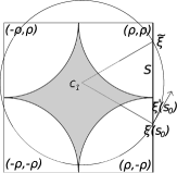
Figure 5. The absurd situation in the proof by contradiction. The circle is $B^{1}(s_{0})$, while the curve is not shown.

Therefore the distance from the origin of the center of $B^{1}(s_{0})$ is less than $\rho$. This implies that $0\in B^{1}(s_{0})$. On the other hand, since $\xi$ is tangent to this disk at $\xi(s_{0})$, the bound on the curvature implies that $\xi(s)\notin B^{1}(s_{0})$ for every $s\in[0,\frac{\pi}{2}]$. This contradicts the assumption $\xi(0)=0$ and concludes the proof of (3.17).

Let $C$ be the curvilinear triangle obtained by removing the disks $B_{\rho}(\pm\rho\,e_{2})$ from the rectangle $(0,\rho)\times(-\rho,\rho)$. Let $C^{+}$ and $C^{-}$ be the parts of $C$ weakly above and strictly below $N(s_{0})$ and let $p$ be the intersection of $N(s_{0})$ and $\partial B_{\rho}(\rho\,e_{2})$ contained in the closure of $C$. Since the distance between $p$ and $\xi(s_{0})$ is less than $2\rho$, we deduce that $p\in B^{1}(s_{0})$. Since $(\rho,\rho)\in B^{1}(s_{0})$ and $\xi(s_{0})\in\partial B^{1}(s_{0})$, we obtain that $C^{+}$ is contained in $B^{1}(s_{0})$.

Let us prove that

$$C^{-}\subset\bigcup_{0\leq s\leq s_{0}}\big{(}B^{1}(s)\cup\{\xi(s)\}\cup B^{2}(s)\big{)}$$

Let us fix $x\in C^{-}$ and let $s_{1}$ be a minimizer of

$$\min_{0\leq s\leq s_{0}}|x-\xi(s)|.$$

Since $\left\langle x,\xi^{\prime}(0)\right\rangle>0$ and $\left\langle x-\xi(s_{0}),\xi^{\prime}(s_{0})\right\rangle<0$, we have $s_{1}\in(0,s_{0})$, hence the orthogonality condition

$$\left\langle x-\xi(s_{1}),\xi^{\prime}(s_{1})\right\rangle=0.$$

Since $|x-\xi(s_{1})|<|x|<2\rho$, the point $x$ belongs to $B^{1}(s_{1})\cup\{\xi(s_{1})\}\cup B^{2}(s_{1})$, which concludes the proof. ∎

We now prove a result stating that a bound on the angle $\vartheta$ formed by the tangent with the first axis implies the non self-intersection of the swimmer.

Lemma 3.8.

Let $\vartheta\in C^{1}([0,L])$, let $\kappa_{0}:=\max\left\{|\vartheta^{\prime}(s)|:s\in[0,L]\right\}$, and let

$$\xi(s)=\int_{0}^{s}\left(\begin{array}[]{c}\cos\vartheta(\sigma)\\ \sin\vartheta(\sigma)\end{array}\right)\mathrm{d}\sigma.$$

Assume $\left\lvert\vartheta(s)\right\rvert<\pi/4$ for every $s\in[0,L]$. Then, $\xi$ satisfies the two disks condition with radius $\rho$, for every $0<\rho\leqslant 1/\kappa_{0}$.

Proof.

Notice, in the first place, that $|\xi^{\prime}(s)|=1$ for every $s\in[0,L]$, so that $\xi$ is a regular curve parametrized by arc length. The condition $|\vartheta(s)|<\pi/4$ for all $s\in[0,L]$ implies that $\xi$ is a graph with respect to the $x_{1}$-axis. Given $\rho$, with $0<\rho\leqslant 1/\kappa_{0}$, we define the open disks $B^{1}(s):=B_{\rho}(\xi(s)+\rho J\xi^{\prime}(s))$ and $B^{2}(s):=B_{\rho}(\xi(s)-\rho J\xi^{\prime}(s))$, as in (3.12). Since $\xi$ is a graph and its curvature is bounded by $\kappa_{0}$, the disks $B^{1}(s)$ and $B^{2}(s)$ satisfy condition (a) in Definition 3.4. Finally, the construction of $B^{-}$ and $B^{+}$ as in condition (b) of Definition 3.4 is straightforward. ∎

The preceding lemma will be useful in Section 4 to check that the deformations we construct to prove the controllability of the swimmer are admissible.

4. Controllability

In this Section we show that the swimmer is controllable, i.e., it is possible to prescribe a self-propelled motion that takes it from a given initial state $\chi_{\mathrm{in}}$ to a given final state $\chi_{\mathrm{fin}}$ . More precisely, we prove the following theorem.

Theorem 4.1.

Let $\rho>0$ and let $\chi_{\mathrm{in}}$ , $\chi_{\mathrm{fin}}\in H^{2}(0,L;\mathbb{R}^{2})$, with $|\chi_{\mathrm{in}}^{\prime}(s)|=|\chi_{\mathrm{fin}}^{\prime}(s)|=1$ for every $s\in[0,L]$. Assume that $\chi_{\mathrm{in}}$ and $\chi_{\mathrm{fin}}$ satisfy the two disks condition with radius $\rho$ (see Definition 3.4). Then, there exists $\chi\in X_{1}$ , satisfying the force and torque balance (2.3), such that $\chi(s,0)=\chi_{\mathrm{in}}(s)$ and $\chi(s,T)=\chi_{\mathrm{fin}}(s)$ for every $s\in[0,L]$, and such that for every $t\in[0,T]$ the curve $\chi(\cdot,t)$ satisfies the two disks condition with radius $\rho$.

Proof.

To construct $\chi$, we divide the interval $[0,T]$ into three intervals $[0,\frac{1}{3}T]$, $[\frac{1}{3}T,\frac{2}{3}T]$, and $[\frac{2}{3}T,T]$. In the first interval we straighten $\chi_{\mathrm{in}}$ , i.e., we construct $\chi$, satisfying the force and torque balance (2.3) and the two disks condition with radius $\rho$ on $[0,\frac{1}{3}T]$, such that $\chi(s,0)=\chi_{\mathrm{in}}(s)$ and $\chi(s,\frac{1}{3}T)=\Sigma_{\mathrm{in}}(s)$ for every $s\in[0,L]$, where $\Sigma_{\mathrm{in}}$ is the arc length parametrization of a suitable segment of length $L$, depending on $\chi_{\mathrm{in}}$ .

The same construction, with time reversed, shows that there exists a segment $\Sigma_{\mathrm{fin}}$, depending on $\chi_{\mathrm{fin}}$ , that can be transferred onto $\chi_{\mathrm{fin}}$ , i.e., there exists $\chi$ satisfying the force and torque balance (2.3) and the the two disks condition with radius $\rho$ on $[\frac{2}{3}T,T]$, such that $\chi(s,\frac{2}{3}T)=\Sigma_{\mathrm{fin}}(s)$ and $\chi(s,T)=\chi_{\mathrm{fin}}(s)$ for every $s\in[0,L]$.

Since, in general, $\Sigma_{\mathrm{fin}}$ does not coincide with $\Sigma_{\mathrm{in}}$ , we use the interval $[\frac{1}{3}T,\frac{2}{3}T]$ to transfer $\Sigma_{\mathrm{in}}$ onto $\Sigma_{\mathrm{fin}}$ .

We now describe the construction of $\chi$ on $[0,\frac{1}{3}T]$. First of all, it is possible to find $\xi\in X_{1}$ such that $\xi(s,0)=\chi_{\mathrm{in}}(s)$ for every $s\in[0,L]$ and $s\mapsto\xi(s,\frac{1}{3}T)$ is affine on $[0,L]$. It is also possible to obtain that $\xi(\cdot,t)$ satisfies the two disks condition with radius $\rho>0$ for every $t\in[0,\frac{1}{3}T]$.

The last requirement can be fulfilled in the following way. If at one end of the swimmer there is enough room, we pull it along the tangent and unwind it from its original shape obtaining a straight configuration, as illustrated in Fig. 6.

Figure 6. Straightening the swimmer I. The dashed line is the straightened configuration.

If this is not the case, then we operate as in Fig. 7: the unwinding is achieved by pinching a point with maximal $x_{1}$-coordinate and pulling it to the right respecting the two disks condition.

Figure 7. Straightening the swimmer II. The dashed lines represent the intermediate phases of the stretching procedure.

We now compose $\xi$ with a time dependent rigid motion and define $\chi$ on $[0,L]\times[0,\frac{1}{3}T]$ by (3.1). Clearly the curve $\chi(\cdot,t)$ continues to satisfy the two disks condition with radius $\rho$ for every $t\in[0,\frac{1}{3}T]$. Moreover the function $\Sigma_{\mathrm{in}}(s):=\chi(s,\frac{1}{3}T)$ is affine and $|\Sigma_{\mathrm{in}}^{\prime}(s)|=1$ for every $s\in[0,L]$. The vector $x$ and the rotation $R$ are chosen so that the equation of motion (3.8) is satisfied (this is possible thanks to Theorem 3.3), so that $\chi$ satisfies the force and torque balance (2.3) in $[0,\frac{1}{3}T]$.

Note that, while the affine map $\xi(\cdot,\frac{1}{3}T)$ can be chosen freely, the corresponding map $\Sigma_{\mathrm{in}}$ depends on the superimposed rigid motion, which, in turn, depends on the data of the problem. Therefore, in this construction the location of the segment $\Sigma_{\mathrm{in}}$ cannot be prescribed.

On $[\frac{2}{3}T,T]$ the function $\chi$ is defined in a similar way. To transfer $\Sigma_{\mathrm{in}}$ into $\Sigma_{\mathrm{fin}}$ in the time interval $[\frac{1}{3}T,\frac{2}{3}T]$ we show that, for a straight swimmer, it is possible to produce self-propelled motions achieving any prescribed translation along its axis and any prescribed rotation about its barycenter.

To summarize, the whole control process is organized as in Fig. 8.

$$\chi_{\mathrm{in}}(\cdot)\xrightarrow{\text{straightening}}\Sigma_{\mathrm{in}}(\cdot)\xrightarrow{\text{rotation, translation, rotation}}\Sigma_{\mathrm{fin}}(\cdot)\xrightarrow{\text{straightening${}^{-1}$}}\chi_{\mathrm{fin}}(\cdot).$$

2pt $\chi_{\mathrm{fin}}$ at 580 50 $\chi_{\mathrm{in}}$ at 18 70 $\Sigma_{\mathrm{fin}}$ at 395 100 $\Sigma_{\mathrm{in}}$ at 200 0 $\downarrow$ at 90 62 $\longrightarrow$ at 460 90 $\longrightarrow$ at 260 45

Figure 8. Sketch of the control process.

4.1. Translation

In this subsection we describe how to translate a straight swimmer along its axis: since the problem is rate independent (see Remark 2.1), it is not restrictive to work in the time interval $[0,1]$. The motion of the swimmer is obtained through the translation along the swimmer itself of a localized bump. In order to get a rectilinear motion, we have to assume that the bump satisfies some symmetry properties (4.10).

We can assume that the swimmer lies initially on the $x_{1}$-axis and that the initial parametrization is $\Sigma_{\mathrm{in}}(s)=se_{1}$ . Given $a\in\mathbb{R}$, we describe a self-propelled motion that transfers the segment $\Sigma_{\mathrm{in}}(s)=se_{1}$ into the segment $\Sigma_{\mathrm{fin}}(s)=(a+s)e_{1}$ , $s\in[0,L]$. It is not restrictive to assume $a>0$.

As before, the motion will be first described through a function $\xi\in X_{1}$ satisfying the two disks condition with the prescribed radius $\rho$. Then, $\xi$ will be composed with a time dependent rigid motion in order to obtain $\chi$ satisfying also the force and torque balance.

For simplicity, we assume $\xi(0,t)=0$ for every $t\in[0,1]$. The function $\xi(s,t)$ will be better described by means of the angle $\vartheta(s,t)$ between its tangent line and the positive $x_{1}$-axis. This leads to the formula

$$\xi(s,t)=\int_{0}^{s}\left(\begin{array}[]{c}\cos\vartheta(\sigma,t)\\ \sin\vartheta(\sigma,t)\end{array}\right)\mathrm{d}\sigma.$$ (4.1)

The function $\vartheta(s,t)$ will be defined using a smooth function $\vartheta_{0}\colon\mathbb{R}\to(-\pi/4,\pi/4)$, with $\max_{s}|\vartheta_{0}^{\prime}(s)|\leqslant 1/\rho$ and support

$$\operatorname{spt}\vartheta_{0}=[-\ell,\ell],\qquad\text{where $\ell\in(0,L/2)$.}$$ (4.2)

Given two Lipschitz continuous control functions $u_{1}:[0,1]\to[-1,1]$ and $u_{2}:[0,1]\to[\ell,L-\ell]$, we define

$$\vartheta(s,t):=u_{1}(t)\vartheta_{0}(s-u_{2}(t)),$$ (4.3)

for every $(s,t)\in[0,L]{\times}[0,1]$. Notice that for all $t\in[0,1]$ the function $\vartheta(\cdot,t)$ has support contained in $[u_{2}(t)-\ell,u_{2}(t)+\ell]$, which in turn is contained in $[0,L]$, and the curve $\xi(\cdot,t)$ satisfies the two disks condition with radius $\rho$ (see Lemma 3.8). The parameters $u_{1}(t)$ and $u_{2}(t)$ represent the amplitude of the bump and the location of its midpoint at time $t$.

It is convenient to introduce the function

$$\xi_{0}(s,u_{1},u_{2}):=\int_{0}^{s}\left(\begin{array}[]{c}\cos(u_{1}\vartheta_{0}(\sigma-u_{2}))\\ \sin(u_{1}\vartheta_{0}(\sigma-u_{2}))\end{array}\right)\,\mathrm{d}\sigma,$$

so that

$$\xi(s,t)=\xi_{0}(s,u_{1}(t),u_{2}(t)).$$ (4.4)

It follows that

$$\xi^{\prime}(s,t)=\xi_{0}^{\prime}(s,u_{1}(t),u_{2}(t)),$$

where

$$\xi_{0}^{\prime}(s,u_{1},u_{2})=\frac{\partial\xi_{0}}{\partial s}(s,u_{1},u_{2})=\left(\begin{array}[]{c}\cos(u_{1}\vartheta_{0}(s-u_{2}))\\ \sin(u_{1}\vartheta_{0}(s-u_{2}))\end{array}\right).$$ (4.5)

Therefore,

$$\begin{split}K_{\xi}(s,t)=&C_{\tau}\xi^{\prime}(s,t)\otimes\xi^{\prime}(s,t)+C_{\nu}(J\xi^{\prime}(s,t))\otimes(J\xi^{\prime}(s,t))\\ =&C_{\tau}\xi_{0}^{\prime}(s,u_{1}(t),u_{2}(t))\otimes\xi_{0}^{\prime}(s,u_{1}(t),u_{2}(t))\\ &+C_{\nu}(J\xi_{0}^{\prime}(s,u_{1}(t),u_{2}(t)))\otimes(J\xi_{0}^{\prime}(s,u_{1}(t),u_{2}(t))).\end{split}$$

It is convenient to introduce

$$K_{0}(s,u_{1},u_{2}):=C_{\tau}\xi_{0}^{\prime}(s,u_{1},u_{2})\otimes\xi_{0}^{\prime}(s,u_{1},u_{2})+C_{\nu}(J\xi_{0}^{\prime}(s,u_{1},u_{2}))\otimes(J\xi_{0}^{\prime}(s,u_{1},u_{2})),$$ (4.6)

so that

$$K_{\xi}(s,t)=K_{0}(s,u_{1}(t),u_{2}(t)).$$ (4.7)

We also have

$$\dot{\xi}(s,t)=\xi_{0,1}(s,u_{1}(t),u_{2}(t))\dot{u}_{1}(t)+\xi_{0,2}(s,u_{1}(t),u_{2}(t))\dot{u}_{2}(t),$$

where

$$\xi_{0,i}(s,u_{1},u_{2}):=\frac{\partial\xi_{0}}{\partial u_{i}}(s,u_{1},u_{2}).$$

A simple computation leads to

$$\xi_{0,1}(s,u_{1},u_{2})=\int_{0}^{s}\left(\begin{array}[]{c}-\sin(u_{1}\vartheta_{0}(\sigma-u_{2}))\\ \cos(u_{1}\vartheta_{0}(\sigma-u_{2}))\end{array}\right)\vartheta_{0}(\sigma-u_{2})\,\mathrm{d}\sigma,$$ (4.8)

$$\begin{split}\xi_{0,2}(s,u_{1},u_{2})=&\int_{0}^{s}\left(\begin{array}[]{c}\sin(u_{1}\vartheta_{0}(\sigma-u_{2}))\\ -\cos(u_{1}\vartheta_{0}(\sigma-u_{2}))\end{array}\right)u_{1}\vartheta_{0}^{\prime}(\sigma-u_{2})\,\mathrm{d}\sigma\\ =&-\int_{0}^{s}\frac{\mathrm{d}}{\mathrm{d}\sigma}\left(\begin{array}[]{c}\cos(u_{1}\vartheta_{0}(\sigma-u_{2}))\\ \sin(u_{1}\vartheta_{0}(\sigma-u_{2}))\end{array}\right)\,\mathrm{d}\sigma\\ =&\left(\begin{array}[]{c}1-\cos(u_{1}\vartheta_{0}(s-u_{2}))\\ -\sin(u_{1}\vartheta_{0}(s-u_{2}))\end{array}\right),\end{split}$$ (4.9)

for every $s\in[0,L]$, $u_{1}\in[-1,1]$, and $u_{2}\in[\ell,L-\ell]$. Note that in the previous computation we have used the fact that $\vartheta_{0}(-u_{2})=0$, since $\operatorname{spt}\vartheta_{0}\subseteq[-\ell,\ell]$.

Finally, we make the following symmetry assumption on the angle function $\vartheta_{0}$:

$$\vartheta_{0}\text{ is odd in $[-\ell,\ell]$};$$ (4.10a)

$$\vartheta_{0}\text{ is even in $[-\ell,0]$ and in $[0,\ell]$};$$ (4.10b)

$$\vartheta_{0}\text{ is odd in $[-\ell,-\ell/2]$, $[-\ell/2,0]$, $[0,\ell/2]$, and in $[\ell/2,\ell]$}.$$ (4.10c)

We say that a function $u\colon[a,b]\to\mathbb{R}$ is said to be even (resp. odd) in $[a,b]$ if $u(x)=u(a+b-x)$ (resp. $u(x)=-u(a+b-x)$) for every $x\in[a,b]$.

Figure 9 shows an example of a bump $\xi_{0}(s,t)$ whose angle function $\vartheta_{0}$ enjoys the properties listed above; notice that the parity of the vertical component of $\xi_{0}$ is reversed with respect to that of $\vartheta_{0}$ .

Figure 9. Image of the function $\xi_{0}(s,t)$ for the translational motion.

To exploit these symmetry properties, we repeatedly use the following lemma, whose elementary proof is omitted.

Lemma 4.2.

Let $u\colon[a,b]\to\mathbb{R}$ be an even (resp. odd) function and let $c:=(a+b)/2$ be the middle point of $[a,b]$. Then, the integral function $U(x):=\int_{c}^{x}u(s)\,\mathrm{d}s$ is odd (resp. even) in $[a,b]$.

We now compose $\xi$ defined in (4.4) with a time dependent rigid motion and define $\chi$ on $[0,L]{\times}[0,1]$ by (3.1). The vector $x(t)$ and the rotation $R(t)$ are chosen so that $x(0)=0$ and $R(0)=I$ and the force and torque balance (2.3) is satisfied by $\chi$ at every time. We want to prove that this is possible with

$$x_{2}(t)=0\quad\text{and}\quad R(t)=I,\qquad\text{for all $t\in[0,1]$},$$ (4.11)

by a suitable choice of $x_{1}(t)$. We shall see that this result follows from the symmetry assumptions (4.10) and does not depend on the particular choice of the control functions $u_{1}(t),u_{2}(t)$.

Note that for every $t\in[0,1]$ we have $\operatorname{spt}\vartheta(\cdot,t)=[u_{2}(t)-\ell,u_{2}(t)+\ell]$. Since $\vartheta(s,t)=0$ for $s\in[0,u_{2}(t)-\ell]$, we obtain from (4.1) that $\xi(s,t)=se_{1}$ for $s\in[0,u_{2}(t)-\ell]$. Similarly, since $\vartheta(s,t)=0$ for every $s\in[u_{2}(t)+\ell,L]$, (4.1) implies that in this interval $\xi(\cdot,t)$ is the arc length parametrization of a segment parallel to the $x_{1}$-axis. Therefore, the curve $\xi(\cdot,t)$ is the union of two segments and a connecting bump, corresponding to the restriction of the curve $\xi(\cdot,t)$ to the interval $[u_{2}(t)-\ell,u_{2}(t)+\ell]$.

Notice that (4.10a) yields $\int_{-\ell}^{\ell}\sin(u_{1}(t)\vartheta_{0}(s))\,\mathrm{d}s=0$, therefore, (4.1) and (4.3) imply that for every $t\in[0,1]$ the curve $s\mapsto\xi(s,t)$, $s\in[u_{2}(t)+\ell,L]$, parametrizes a segment lying on the $x_{1}$-axis. Moreover, by a change of variables we have

$$\xi(u_{2}(t)+\ell,t)-\xi(u_{2}(t)-\ell,t)=\int_{-\ell}^{\ell}\left(\begin{array}[]{c}\cos(u_{1}(t)\vartheta_{0}(s))\\ \sin(u_{1}(t)\vartheta_{0}(s))\end{array}\right)\mathrm{d}s=\left(\int_{-\ell}^{\ell}\cos(u_{1}(t)\vartheta_{0}(s))\,\mathrm{d}s\right)e_{1}.$$

These two remarks imply that

$$\xi(s,t)=\left(s-2l+\int_{-\ell}^{\ell}\cos(u_{1}(t)\vartheta_{0}(s))\,\mathrm{d}s\right)e_{1},\qquad\text{for }u_{2}(t)+\ell\leqslant s\leqslant L.$$

Using (3.1) and (4.11), the expression for $\chi$ reads $\chi(s,t)=x_{1}(t)e_{1}+\xi(s,t)$. From this we get $\chi^{\prime}(s,t)=\xi^{\prime}(s,t)$ and $\dot{\chi}(s,t)=\dot{x}_{1}(t)e_{1}+\dot{\xi}(s,t)$. It follows that the matrix $K_{\chi}$ defined in (2.2) satisfies

$$K_{\chi}(s,t)=K_{\xi}(s,t)=C_{\tau}\xi^{\prime}(s,t)\otimes\xi^{\prime}(s,t)+C_{\nu}(J\xi^{\prime}(s,t))\otimes(J\xi^{\prime}(s,t)).$$

The linear densities of force and moment (see (2.1)) are then given by

$$\begin{split}-f(s,t)=&\,\,K_{\chi}(s,t)\dot{\chi}(s,t)=\dot{x}_{1}(t)K_{\xi}(s,t)e_{1}+K_{\xi}(s,t)\dot{\xi}(s,t)\\ -m(s,t)=&\,\,\dot{x}_{1}(t)\langle K_{\xi}(s,t)e_{1},J\xi(s,t)\rangle+\dot{x}_{1}(t)x_{1}(t)\left\langle K_{\xi}(s,t)e_{1},e_{2}\right\rangle\\ &\,\,+\langle K_{\xi}(s,t)\dot{\xi}(s,t),J\xi(s,t)\rangle+x_{1}(t)\langle K_{\xi}(s,t)\dot{\xi}(s,t),e_{2}\rangle\end{split}$$

By plugging this information in (2.3), we get

$$\dot{x}_{1}(t)\int_{0}^{L}K_{\xi}(s,t)e_{1}\,\mathrm{d}s=-\int_{0}^{L}K_{\xi}(s,t)\dot{\xi}(s,t)\,\mathrm{d}s,$$ (4.12)

where the right-hand side is $F^{\mathrm{sh}}(t)$ defined in (3.7), and

$$\begin{split}\dot{x}_{1}(t)&\int_{0}^{L}\langle K_{\xi}(s,t)e_{1},J\xi(s,t)\rangle\mathrm{d}s+\dot{x}_{1}(t)x_{1}(t)\int_{0}^{L}\left\langle K_{\xi}(s,t)e_{1},e_{2}\right\rangle\mathrm{d}s=\\ &-\int_{0}^{L}\langle K_{\xi}(s,t)\dot{\xi}(s,t),J\xi(s,t)\rangle\,\mathrm{d}s-x_{1}(t)\int_{0}^{L}\langle K_{\xi}(s,t)\dot{\xi}(s,t),e_{2}\rangle\,\mathrm{d}s.\end{split}$$ (4.13)

To solve simultaneously these equations for the unknown $\dot{x}_{1}(t)$, we will show that the second components of the integrals in (4.12) are zero, that the first component of the integral in the left-hand side in (4.12) is non zero, and that all integrals in (4.13) are zero.

Let us start from the second components of (4.12). For the left-hand side, we have

$$\begin{split}\left\langle K_{\xi}(s,t)e_{1},e_{2}\right\rangle=&\left\langle K_{0}(s,u_{1}(t),u_{2}(t))e_{1},e_{2}\right\rangle\\ =&(C_{\tau}-C_{\nu})\cos(u_{1}(t)\vartheta_{0}(s-u_{2}(t)))\sin(u_{1}(t)\vartheta_{0}(s-u_{2}(t)))\end{split}$$

so it suffices to show that for every $u_{1},u_{2}$

$$\int_{0}^{L}\cos(u_{1}\vartheta_{0}(s-u_{2}))\sin(u_{1}\vartheta_{0}(s-u_{2}))\,\mathrm{d}s=0.$$ (4.14)

By (4.2) and by changing variables $\sigma=s-u_{2}$, (4.14) becomes

$$\int_{-\ell}^{\ell}\cos(u_{1}\vartheta_{0}(\sigma))\sin(u_{1}\vartheta_{0}(\sigma))\,\mathrm{d}\sigma=0,$$

which holds true since the integrand is an odd function in $[-\ell,\ell]$, thanks to (4.10a).

For the second component of the right-hand side of (4.12), we have

$$\begin{split}\langle K_{\xi}(s,t)&\dot{\xi}(s,t),e_{2}\rangle=C_{\tau}\dot{u}_{1}(t)\sin(u_{1}(t)\vartheta_{0}(s-u_{2}(t)))\cdot\\ &\cdot\left[-\cos(u_{1}(t)\vartheta_{0}(s-u_{2}(t)))\int_{0}^{s}\sin(u_{1}(t)\vartheta_{0}(\sigma-u_{2}(t)))\vartheta_{0}(\sigma-u_{2}(t))\,\mathrm{d}\sigma\right.\\ &\quad\left.+\sin(u_{1}(t)\vartheta_{0}(s-u_{2}(t)))\int_{0}^{s}\cos(u_{1}(t)\vartheta_{0}(\sigma-u_{2}(t)))\vartheta_{0}(\sigma-u_{2}(t))\,\mathrm{d}\sigma\right]\\ &-C_{\nu}\dot{u}_{2}(t)\cos(u_{1}(t)\vartheta_{0}(s-u_{2}(t)))\sin(u_{1}(t)\vartheta_{0}(s-u_{2}(t))).\end{split}$$

Therefore, we need to prove that for any $u_{1},u_{2}$

$$\int_{0}^{L}\sin(2u_{1}\vartheta_{0}(s-u_{2}))\left[\int_{0}^{s}\sin(u_{1}\vartheta_{0}(\sigma-u_{2}))\vartheta_{0}(\sigma-u_{2})\,\mathrm{d}\sigma\right]\mathrm{d}s=0,$$ (4.15)

$$\int_{0}^{L}\sin^{2}(u_{1}\vartheta_{0}(s-u_{2}))\left[\int_{0}^{s}\cos(u_{1}\vartheta_{0}(\sigma-u_{2}))\vartheta_{0}(\sigma-u_{2})\,\mathrm{d}\sigma\right]\mathrm{d}s=0.$$ (4.16)

Again by (4.2) and by changing variables as before, (4.15) and (4.16) reduce to

$$\int_{-\ell}^{\ell}\sin(2u_{1}\vartheta_{0}(s))\left[\int_{-\ell}^{s}\sin(u_{1}\vartheta_{0}(\sigma))\vartheta_{0}(\sigma)\,\mathrm{d}\sigma\right]\mathrm{d}s=0,$$ (4.17)

$$\int_{-\ell}^{\ell}\sin^{2}(u_{1}\vartheta_{0}(s))\left[\int_{-\ell}^{s}\cos(u_{1}\vartheta_{0}(\sigma))\vartheta_{0}(\sigma)\,\mathrm{d}\sigma\right]\mathrm{d}s=0.$$ (4.18)

Since $\sin(2u_{1}\vartheta_{0}(s))$ is odd in $[-\ell,\ell]$ by (4.10a), equation (4.17) is equivalent to

$$\int_{-\ell}^{\ell}\sin(2u_{1}\vartheta_{0}(s))\left[\int_{0}^{s}\sin(u_{1}\vartheta_{0}(\sigma))\vartheta_{0}(\sigma)\,\mathrm{d}\sigma\right]\mathrm{d}s=0.$$ (4.19)

By (4.10a) and by Lemma 4.2 the function $s\mapsto\int_{0}^{s}\sin(u_{1}\vartheta_{0}(\sigma))\vartheta_{0}(\sigma)\,\mathrm{d}\sigma$ is odd in $[-\ell,\ell]$, therefore (4.19) is equivalent to

$$\int_{0}^{\ell}\sin(2u_{1}\vartheta_{0}(s))\left[\int_{0}^{s}\sin(u_{1}\vartheta_{0}(\sigma))\vartheta_{0}(\sigma)\,\mathrm{d}\sigma\right]\mathrm{d}s=0,$$ (4.20)

since its integrand is even in $[-\ell,\ell]$. Since $\sin(2u_{1}\vartheta_{0}(s))$ is even in $[0,\ell]$ by (4.10b), we have

$$\int_{0}^{\ell}\sin(2u_{1}\vartheta_{0}(s))\,\mathrm{d}s=2\int_{0}^{\ell/2}\sin(2u_{1}\vartheta_{0}(s))\,\mathrm{d}s=0,$$

where the last equality follows from the fact that $\sin(2u_{1}\vartheta_{0}(s))$ is odd in $[0,\ell/2]$ by (4.10c). This equality implies that (4.20) reduces to

$$\int_{0}^{\ell}\sin(2u_{1}\vartheta_{0}(s))\left[\int_{\ell/2}^{s}\sin(u_{1}\vartheta_{0}(\sigma))\vartheta_{0}(\sigma)\,\mathrm{d}\sigma\right]\mathrm{d}s=0.$$ (4.21)

By (4.10b), $\sin(2u_{1}\vartheta_{0}(s))$, and $\sin(u_{1}\vartheta_{0}(s))\vartheta_{0}(s)$ are even in $[0,\ell]$, hence the function $s\mapsto\int_{\ell/2}^{s}\sin(u_{1}\vartheta_{0}(\sigma))\vartheta_{0}(\sigma)\,\mathrm{d}\sigma$ is odd in $[0,\ell]$ by Lemma 4.2. This implies that (4.21) holds, since its integrand is odd in $[0,\ell]$. This concludes the proof of (4.17).

To prove (4.18) we notice that in the function $s\mapsto\cos(u_{1}\vartheta_{0}(s))\vartheta_{0}(s)$ is even in $[-\ell,0]$ by (4.10b). Hence,

$$\int_{-\ell}^{0}\cos(u_{1}\vartheta_{0}(\sigma))\vartheta_{0}(\sigma)\,\mathrm{d}\sigma=2\int_{-\ell/2}^{0}\cos(u_{1}\vartheta_{0}(\sigma))\vartheta_{0}(\sigma)\,\mathrm{d}\sigma=0,$$ (4.22)

where the last equality follows from the fact that the function $s\mapsto\cos(u_{1}\vartheta_{0}(s))\vartheta_{0}(s)$ is odd in $[-\ell/2,0]$ by (4.10c). This implies that (4.18) is equivalent to

$$\int_{-\ell}^{\ell}\sin^{2}(u_{1}\vartheta_{0}(s))\left[\int_{0}^{s}\cos(u_{1}\vartheta_{0}(\sigma))\vartheta_{0}(\sigma)\,\mathrm{d}\sigma\right]\mathrm{d}s=0.$$ (4.23)

By (4.10a), the function $\cos(u_{1}\vartheta_{0}(\sigma))\vartheta_{0}(\sigma)$ is odd in $[-\ell,\ell]$, and therefore the function $s\mapsto\int_{0}^{s}\cos(u_{1}\vartheta_{0}(\sigma))\vartheta_{0}(\sigma)\,\mathrm{d}\sigma$ is even in $[-\ell,\ell]$ by Lemma 4.2. Since also $\sin^{2}(u_{1}\vartheta_{0}(s))$ is even in $[-\ell,\ell]$ by (4.10a), (4.23) is equivalent to

$$\int_{0}^{\ell}\sin^{2}(u_{1}\vartheta_{0}(s))\left[\int_{0}^{s}\cos(u_{1}\vartheta_{0}(\sigma))\vartheta_{0}(\sigma)\,\mathrm{d}\sigma\right]\mathrm{d}s=0,$$

which, by (4.22), is equivalent to

$$\int_{0}^{\ell}\sin^{2}(u_{1}\vartheta_{0}(s))\left[\int_{\ell/2}^{s}\cos(u_{1}\vartheta_{0}(\sigma))\vartheta_{0}(\sigma)\,\mathrm{d}\sigma\right]\mathrm{d}s=0.$$ (4.24)

By (4.10b), the function $\cos(u_{1}\vartheta_{0}(\sigma))\vartheta_{0}(\sigma)$ is even in $[0,\ell]$, and therefore the function $s\mapsto\int_{\ell/2}^{s}\cos(u_{1}\vartheta_{0}(\sigma))\vartheta_{0}(\sigma)\,\mathrm{d}\sigma$ is odd in $[0,\ell]$ by Lemma 4.2. Since also $\sin^{2}(u_{1}\vartheta_{0}(s))$ is even in $[0,\ell]$ by (4.10b), (4.24) holds because its integrand is odd in $[0,\ell]$. This concludes the proof of (4.18). Therefore, we have proved that the second component in (4.12) vanishes.

By the results just proved, (4.13) reduces to

$$\dot{x}_{1}(t)\int_{0}^{L}\langle K_{\xi}(s,t)e_{1},J\xi(s,t)\rangle\mathrm{d}s=-\int_{0}^{L}\langle K_{\xi}(s,t)\dot{\xi}(s,t),J\xi(s,t)\rangle\,\mathrm{d}s$$ (4.25)

To prove that the left-hand side is zero, by (4.6) and (4.7) it is enough to show that

$$\int_{0}^{L}\left\langle\xi_{0}^{\prime}(s,t),e_{1}\right\rangle\left\langle\xi_{0}^{\prime}(s,t),J\xi_{0}(s,t)\right\rangle\,\mathrm{d}s=\int_{0}^{L}\left\langle J\xi_{0}^{\prime}(s,t),e_{1}\right\rangle\left\langle J\xi_{0}^{\prime}(s,t),J\xi_{0}(s,t)\right\rangle\,\mathrm{d}s=0,$$

which in turn is valid if we prove that, for any $u_{1},u_{2}$ (after recalling (4.2) and performing the usual change of variables $s-u_{2}\to s$)

$$\int_{-\ell}^{\ell}\sin(2u_{1}\vartheta_{0}(s))\left[\int_{-\ell}^{s}\cos(u_{1}\vartheta_{0}(\sigma))\,\mathrm{d}\sigma\right]\mathrm{d}s=0,$$

$$\int_{-\ell}^{\ell}\sin^{2}(u_{1}\vartheta_{0}(s))\left[\int_{-\ell}^{s}\sin(u_{1}\vartheta_{0}(\sigma))\,\mathrm{d}\sigma\right]\mathrm{d}s=0,$$

$$\int_{-\ell}^{\ell}\cos^{2}(u_{1}\vartheta_{0}(s))\left[\int_{-\ell}^{s}\sin(u_{1}\vartheta_{0}(\sigma))\,\mathrm{d}\sigma\right]\mathrm{d}s=0.$$

To prove these equalities we can argue as in (4.17) and (4.18).

To prove that the right-hand side of (4.25) is zero, besides the equalities already proved, we have to show that

$$\int_{-\ell}^{\ell}\cos(u_{1}\vartheta_{0}(s))\left[\int_{-\ell}^{s}\sin(u_{1}\vartheta_{0}(\sigma))\,\mathrm{d}\sigma\right]\mathrm{d}s=0,$$

$$\int_{-\ell}^{\ell}\sin(u_{1}\vartheta_{0}(s))\left[\int_{-\ell}^{s}\cos(u_{1}\vartheta_{0}(\sigma))\,\mathrm{d}\sigma\right]\mathrm{d}s=0,$$

$$\int_{-\ell}^{\ell}\cos^{2}(u_{1}\vartheta_{0}(s))\left[\int_{-\ell}^{s}\sin(u_{1}\vartheta_{0}(\sigma))\vartheta_{0}(\sigma)\,\mathrm{d}\sigma\right]\!\!\left[\int_{-\ell}^{s}\sin(u_{1}\vartheta_{0}(\sigma))\,\mathrm{d}\sigma\right]\mathrm{d}s=0,$$

$$\int_{-\ell}^{\ell}\sin^{2}(u_{1}\vartheta_{0}(s))\left[\int_{-\ell}^{s}\sin(u_{1}\vartheta_{0}(\sigma))\vartheta_{0}(\sigma)\,\mathrm{d}\sigma\right]\!\!\left[\int_{-\ell}^{s}\sin(u_{1}\vartheta_{0}(\sigma))\,\mathrm{d}\sigma\right]\mathrm{d}s=0,$$

$$\int_{-\ell}^{\ell}\!\!\sin(2u_{1}\vartheta_{0}(s))\!\left[\int_{-\ell}^{s}\!\!\sin(u_{1}\vartheta_{0}(\sigma))\vartheta_{0}(\sigma)\,\mathrm{d}\sigma\right]\!\!\left[\int_{-\ell}^{s}\!\!\cos(u_{1}\vartheta_{0}(\sigma))\,\mathrm{d}\sigma\right]\mathrm{d}s=0,$$

$$\int_{-\ell}^{\ell}\!\!\sin(2u_{1}\vartheta_{0}(s))\!\left[\int_{-\ell}^{s}\!\!\cos(u_{1}\vartheta_{0}(\sigma))\vartheta_{0}(\sigma)\,\mathrm{d}\sigma\right]\!\!\left[\int_{-\ell}^{s}\!\!\sin(u_{1}\vartheta_{0}(\sigma))\,\mathrm{d}\sigma\right]\mathrm{d}s=0,$$

$$\int_{-\ell}^{\ell}\sin^{2}(u_{1}\vartheta_{0}(s))\left[\int_{-\ell}^{s}\cos(u_{1}\vartheta_{0}(\sigma))\vartheta_{0}(\sigma)\,\mathrm{d}\sigma\right]\!\!\left[\int_{-\ell}^{s}\cos(u_{1}\vartheta_{0}(\sigma))\,\mathrm{d}\sigma\right]\mathrm{d}s=0,$$

$$\int_{-\ell}^{\ell}\cos^{2}(u_{1}\vartheta_{0}(s))\left[\int_{-\ell}^{s}\cos(u_{1}\vartheta_{0}(\sigma))\vartheta_{0}(\sigma)\,\mathrm{d}\sigma\right]\!\!\left[\int_{-\ell}^{s}\cos(u_{1}\vartheta_{0}(\sigma))\,\mathrm{d}\sigma\right]\mathrm{d}s=0.$$

This can be done as in the previous proofs, using the symmetry assumptions (4.10) together with Lemma 4.2.

We still need to verify that the first component in the left-hand side of (4.12) does not vanish. Indeed, by using (4.5), (4.6), and (4.7),

$$\begin{split}\int_{0}^{L}\left\langle K_{\xi}(s,t)e_{1},e_{1}\right\rangle\mathrm{d}s=&\int_{-\ell}^{\ell}[C_{\tau}\cos^{2}(u_{1}\vartheta_{0}(s))+C_{\nu}\sin^{2}(u_{1}\vartheta_{0}(s))]\mathrm{d}s,\end{split}$$

which is clearly greater than zero. Therefore, (4.12) can be written in the following way

$$\dot{x}_{1}(t)=\frac{F^{\mathrm{sh}}(t)}{b(u_{1}(t))}=a_{1}(u_{1}(t))\dot{u}_{1}(t)+a_{2}(u_{1}(t))\dot{u}_{2}(t),$$ (4.26)

where we have set

$$a_{i}(u_{1}) := -\frac{b_{i}(u_{1})}{b(u_{1})},$$ (4.27a)

$$b(u_{1}) := \int_{0}^{L}\left\langle K_{0}(s,u_{1},u_{2})e_{1},e_{1}\right\rangle\mathrm{d}s,$$ (4.27b)

$$b_{i}(u_{1}) := \int_{0}^{L}\left\langle K_{0}(s,u_{1},u_{2})\xi_{0,i}(s,u_{1},u_{2}),e_{1}\right\rangle\mathrm{d}s,$$ (4.27c)

since the right-hand sides in (4.27) are in fact independent of $u_{2}$. Indeed, an easy computation recalling (4.6), (4.8), and (4.9) leads to the following expressions

$$b(u_{1}) = 2C_{\tau}\ell+(C_{\nu}-C_{\tau})\int_{-\ell}^{\ell}\sin^{2}(u_{1}\vartheta_{0}(s))\,\mathrm{d}s,$$ (4.28a)

$$b_{1}(u_{1}) = -C_{\tau}\int_{-\ell}^{\ell}\left[\int_{-\ell}^{s}\vartheta_{0}(\sigma)\sin(u_{1}\vartheta_{0}(\sigma))\mathrm{d}\sigma\right]\mathrm{d}s$$

$$-(C_{\nu}-C_{\tau})\int_{-\ell}^{\ell}\sin^{2}(u_{1}\vartheta_{0}(s))\left[\int_{-\ell}^{s}\vartheta_{0}(\sigma)\sin(u_{1}\vartheta_{0}(\sigma))\mathrm{d}\sigma\right]\mathrm{d}s$$

$$+\frac{C_{\tau}-C_{\nu}}{2}\int_{-\ell}^{\ell}\sin(2u_{1}\vartheta_{0}(s))\left[\int_{-\ell}^{s}\vartheta(\sigma)\cos(u_{1}\vartheta_{0}(\sigma))\mathrm{d}\sigma\right]\mathrm{d}s$$

$$b_{2}(u_{1}) = 2C_{\tau}\ell-C_{\tau}\!\!\int_{-\ell}^{\ell}\!\!\cos(u_{1}\vartheta_{0}(s))\mathrm{d}s{+}(C_{\nu}-C_{\tau})\!\!\int_{-\ell}^{\ell}\!\!\sin^{2}(u_{1}\vartheta_{0}(s))\mathrm{d}s.$$ (4.28c)

Notice that from (4.12) and (4.26)

$$F^{\mathrm{sh}}(t)=[b_{1}(u_{1}(t))\dot{u}_{1}(t)+b_{2}(u_{1}(t))\dot{u}_{2}(t)]e_{1}.$$ (4.29)

Assume that $u_{1}(0)=0$. Since $x_{1}(0)=0$ and $\xi(0,0)=0$ (recall that we have assumed $x(0)=0$ and $\xi(0,t)=0$ for all $t\in[0,1]$), the initial condition $\chi(\cdot,0)=\Sigma_{\mathrm{in}}(\cdot)$ is satisfied.

Assume also that $u_{1}(1)=0$. Since $\xi(0,1)=0$, the final condition $\chi(\cdot,1)=\Sigma_{\mathrm{fin}}(\cdot)$ is satisfied provided $x_{1}(1)=a$. Therefore we have to show that we can choose the Lipschitz controls $u_{1}:[0,1]\to[-1,1]$ and $u_{2}:[0,1]\to[\ell,L-\ell]$ in such a way that the corresponding solution of (4.26) satisfying the initial conditions $x_{1}(0)=0$ satisfies also the final condition $x_{1}(1)=a$.

Equation (4.26) shows that $x_{1}(1)$ is the integral of the differential form $a_{1}(u_{1})\mathrm{d}u_{1}+a_{2}(u_{1})\mathrm{d}u_{2}$ along the oriented curve $t\mapsto\left(\begin{array}[]{c}u_{1}(t)\\ u_{2}(t)\end{array}\right)$.

We shall prove that there exists $\delta\in(0,1)$ such that

$$\frac{\mathrm{d}a_{2}}{\mathrm{d}u_{1}}(0)=0\qquad\text{and}\qquad\frac{\mathrm{d}a_{2}}{\mathrm{d}u_{1}}(u_{1})<0,\qquad\text{for $0<u_{1}<\delta$.}$$ (4.30)

For every $\gamma\leqslant\delta$, let us consider the rectangle $\mathcal{R}_{\gamma}:=[0,\gamma]{\times}[\ell,L-\ell]$. If $(u_{1}^{\gamma}(t),u_{2}^{\gamma}(t))$ is a clockwise parametrization of $\partial\mathcal{R}_{\gamma}$ with $u_{1}^{\gamma}(0)=u_{1}^{\gamma}(1)=0$, then the corresponding solutions $x_{1}^{\gamma}$ to (4.26) with initial condition $x_{1}^{\gamma}(0)=0$ satisfy the condition

$$0<x_{1}^{\gamma}(1)\leqslant x_{1}^{\delta}(1).$$

If $0<a\leqslant x_{1}^{\delta}(1)$, by continuity there exists $\gamma\in(0,\delta]$ such that $x_{1}^{\gamma}(1)=a$. If $a>x_{1}^{\delta}(1)$, then we can write $a=nb$, with $n\in\mathbb{N}$ and $b\in(0,x_{1}^{\delta}(1)]$, and fix $\gamma$ such that $x_{1}^{\gamma}(1)=b$. We then extend $u_{1}$ and $u_{2}$ by $1$-periodicity, and we achieve the equality $x_{1}(1)=a$ by choosing as control $(u_{1}(t),u_{2}(t))=(u_{1}^{\gamma}(nt),u_{2}^{\gamma}(nt))$.

We remark that this elementary argument, based on the non-integrability of the differential form $a_{1}(u_{1})\mathrm{d}u_{1}+a_{2}(u_{1})\mathrm{d}u_{2}$, is a particular case of a well know result in Geometric Control Theory, namely Chow’s Theorem, see, e.g., [9, Theorem 3.18].

We now prove (4.30). By (4.28a) and (4.28c) it is easy to compute

$$\begin{split}\frac{\mathrm{d}b}{\mathrm{d}u_{1}}(u_{1})=&(C_{\nu}-C_{\tau})\int_{-\ell}^{\ell}\sin(2u_{1}\vartheta_{0}(s))\vartheta_{0}(s)\,\mathrm{d}s,\\ \frac{\mathrm{d}b_{2}}{\mathrm{d}u_{1}}(u_{1})=&C_{\tau}\int_{-\ell}^{\ell}\sin(u_{1}\vartheta_{0}(s))\vartheta_{0}(s)\mathrm{d}s+(C_{\nu}-C_{\tau})\int_{-\ell}^{\ell}\sin(2u_{1}\vartheta_{0}(s))\vartheta_{0}(s)\mathrm{d}s,\end{split}$$ (4.31)

$$b(0)=2C_{\tau}\ell,\qquad b_{2}(0)=0,\qquad\frac{\mathrm{d}b}{\mathrm{d}u_{1}}(0)=0,\qquad\frac{\mathrm{d}b_{2}}{\mathrm{d}u_{1}}(0)=0,$$ (4.32)

which implies the first equality in (4.30), since

$$b^{2}(u_{1})\frac{\mathrm{d}a_{2}}{\mathrm{d}u_{1}}(u_{1})=-\frac{\mathrm{d}b_{2}(u_{1})}{\mathrm{d}u_{1}}b(u_{1})+b_{2}(u_{1})\frac{\mathrm{d}b(u_{1})}{\mathrm{d}u_{1}}.$$ (4.33)

To establish the result on the sign of $\frac{\mathrm{d}a_{2}}{\mathrm{d}u_{1}}(u_{1})$, it is enough to study the derivative of the right-hand side of (4.33), which is equal to

$$-\frac{\mathrm{d}^{2}b_{2}}{\mathrm{d}u_{1}^{2}}(u_{1})b(u_{1})+b_{2}(u_{1})\frac{\mathrm{d}^{2}b}{\mathrm{d}u_{1}^{2}}(u_{1}).$$ (4.34)

From (4.31) we obtain

$$\begin{split}\frac{\mathrm{d}^{2}b_{2}}{\mathrm{d}u_{1}^{2}}(u_{1})=&C_{\tau}\int_{-\ell}^{\ell}\cos(u_{1}\vartheta_{0}(s))\vartheta_{0}^{2}(s)\mathrm{d}s+2(C_{\nu}-C_{\tau})\int_{-\ell}^{\ell}\cos(2u_{1}\vartheta_{0}(s))\vartheta_{0}^{2}(s)\mathrm{d}s,\end{split}$$

and therefore

$$\frac{\mathrm{d}^{2}b_{2}}{\mathrm{d}u_{1}^{2}}(0)=(2C_{\nu}-C_{\tau})\int_{-\ell}^{\ell}\vartheta_{0}^{2}(s)\mathrm{d}s.$$

Evaluating (4.34) at $u_{1}=0$ gives (recall the second equality in (4.32))

$$\operatorname{sign}\left(\frac{\mathrm{d}^{2}a_{2}}{\mathrm{d}u_{1}^{2}}(0)\right)=\operatorname{sign}\left(-2C_{\tau}\ell(2C_{\nu}-C_{\tau})\int_{-\ell}^{\ell}\vartheta_{0}^{2}(s)\mathrm{d}s\right)<0,$$

which proves the second part of claim (4.30).

4.2. Rotation

In this subsection we describe how to rotate a straight swimmer about its center in the time interval $[0,1]$. This will be obtained in three steps. In the first one we deform symmetrically the initial segment into the shape in Fig. 10, with two parallel straight terminal parts; by symmetry the deformation process will produce a rotation of an angle $\varphi_{0}$ (that we will not estimate) about the midpoint. In the second step we propagate bumps on the rectilinear parts as described below in order to achieve a rotation of a prescribed angle $\varphi$. In the third step, we straighten back the now rotated configuration in Fig. 10 into a straight one by reverting the process in step one: this will produce a rotation of angle $-\varphi_{0}$ about the midpoint, so that at the end of the process the segment will be rotated by the angle $\varphi$.

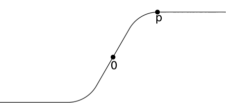
Figure 10. Rotation: the configurations $\xi(s,1/3)=\xi(s,2/3)$.

Without loss of generality, in this section it is convenient to assume that the length of the swimmer is $2L$ and to parametrize all curves in the interval $[-L,L]$. We take $\Sigma_{\mathrm{in}}(s)=se_{1}$ and $\Sigma_{\mathrm{fin}}(s)=se(\varphi)$, for $s\in[-L,L]$, where $e(\varphi)=(\cos\varphi,\sin\varphi)$, $\varphi$ being the angle of rotation. As before, the motion will be first described through a function $\xi\in X_{1}$ satisfying the two disks condition with radius $\rho$. Then, we will consider the function $\chi(s,t)$ defined by (3.1), where $x(t)$ and $R(t)$ satisfy the equation of motion (3.8). The initial and final conditions on $\chi$ are

$$\chi(s,0)=se_{1}\,,\qquad\chi(s,1)=se(\varphi),$$ (4.35)

for all $s\in[-L,L]$.

We also assume that $\xi(s,0)=se_{1}$ and that $\xi$ satisfies

$$\xi(s,t)=-\xi(-s,t)$$ (4.36)

for every $s\in[-L,L]$ and for every $t\in[0,1]$. It follows that

$$\xi^{\prime}(s,t)=\xi^{\prime}(-s,t),\qquad\qquad\dot{\xi}(s,t)=-\dot{\xi}(-s,t),$$ (4.37)

which implies that the force density $f(s,t)$ in (2.1) is odd with respect to $s$, so that $F(t)=\int_{-L}^{L}f(s,t)\,\mathrm{d}s=0$ for all $t\in[0,1]$.

The quantities introduced in (3.6), (3.7), and (3.9) are now defined by integration over the interval $[-L,L]$. The symmetry properties (4.36) and (4.37) imply also that the vector $b(t)$ introduced in (3.6a) and the vector $F^{\mathrm{sh}}(t)$ defined in (3.7) vanish. As a consequence, the vectors $\bar{b}(t)$ and $v(t)$ introduced in (3.9) are zero and $\bar{c}(t)=1/c(t)$. Therefore, the equations of motion (3.8) read $\dot{x}(t)=0$ and

$$\dot{\theta}(t)=\omega(t):=\frac{M^{\mathrm{sh}}(t)}{c(t)},$$ (4.38)

where $\theta(t)$ is the angle of the rotation $R(t)$. Together with the initial conditions at time $t=0$, this implies that $x(t)=0$ for every $t\in[0,1]$, $\theta(0)=0$, and

$$\chi(s,t)=R(t)\xi(s,t).$$

Therefore, the final condition in (4.35) is equivalent to

$$\theta(1)\equiv\varphi\mod 2\pi.$$

The first step will take place in the time interval $[0,1/3]$. The curve $\xi(\cdot,1/3)$ is the one represented in Fig. 10. The main feature of this curve, besides being odd, is that $\xi(s,1/3)=p+(s-L/2)e_{1}$, for $s\in[L/2,L]$, where $p=\xi(L/2,1/3)$ and $p_{2}>0$. The angle $\varphi_{0}$ mentioned at the beginning of the section is then defined by $\varphi_{0}=\theta(1/3)$.

The second step will take place in the time interval $[1/3,2/3]$. As in the case of pure translations, the overall rotation of angle $\varphi$ will be achieved by iterating the cyclic motions described below.

During each cycle, we deform the rectilinear parts of the swimmer with the same bumps we used for the translation, see Fig. 11.

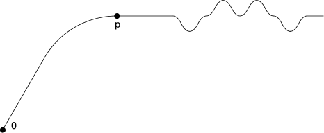
Figure 11. Rotation: the right half of the swimmer is shown, $s\in[0,L]$.

They will be created at the ends of the swimmer, will travel towards its center, and will be destroyed before entering the curvilinear part.

To describe the geometry of the bumps, we use the angle function $\vartheta(s,t)$ considered in (4.3), where now the Lipschitz controls $u_{1}$ and $u_{2}$ take values in $[-1,1]$ and $[L/2+\ell,L-\ell]$, with $\ell\in(0,L/4)$. The corresponding function $\xi(s,t)$ is defined by $\xi(s,t)=\xi(s,1/3)$ for $s\in[0,L/2]$ and $t\in[1/3,2/3]$, and by $\xi(s,t)=\xi_{0}(s,u_{1}(t),u_{2}(t))$, where

$$\xi_{0}(s,u_{1},u_{2}):=p+\int_{L/2}^{s}\left(\begin{array}[]{c}\cos(u_{1}\vartheta_{0}(\sigma-u_{2}))\\ \sin(u_{1}\vartheta_{0}(\sigma-u_{2}))\end{array}\right)\mathrm{d}\sigma.$$

Using (4.29), the force $F^{\mathrm{sh}}(t)$ generated during the translation of the bumps is given by

$$F_{\mathrm{right}}^{\mathrm{sh}}(t)=[b_{1}(u_{1}(t))\dot{u}_{1}(t)+b_{2}(u_{1}(t))\dot{u}_{2}(t)]e_{1},\qquad\text{for every $t\in[1/3,2/3]$.}$$

By the symmetries introduced in (4.36), the global torque defined in (3.7) can be computed as

$$\begin{split}M^{\mathrm{sh}}(t)=&-2\int_{L/2}^{L}\langle J(\xi(s,t)-p),K_{\xi}(s,t)\dot{\xi}(s,t)\rangle\,\mathrm{d}s+2\left\langle Jp,F_{\mathrm{right}}^{\mathrm{sh}}(t)\right\rangle\\ =&-2p_{2}[b_{1}(u_{1}(t))\dot{u}_{1}(t)+b_{2}(u_{1}(t))\dot{u}_{2}(t)]\end{split}$$

where the integral, which represents the torque with respect to the point $p$, vanishes, as explained in Section 4.1.

To compute $\dot{\theta}(t)$ in (4.38), it is convenient to write

$$c(t)=b^{*}(u_{1}(t)),$$

where, by (3.6b), (4.36), and (4.37)

$$b^{*}(u_{1}):=2C_{\tau}\int_{L/2}^{L}\left\langle\xi_{0}^{\prime}(s,u_{1},u_{2}),J\xi_{0}(s,u_{1},u_{2})\right\rangle^{2}\mathrm{d}s+2C_{\nu}\int_{L/2}^{L}\left\langle\xi_{0}^{\prime}(s,u_{1},u_{2}),\xi_{0}(s,u_{1},u_{2})\right\rangle^{2}\mathrm{d}s;$$

it is easy to see that the right-hand side above is independent of $u_{2}$. Equation (4.38) becomes now

$$\dot{\theta}(t)=a_{1}^{*}(u_{1}(t))\dot{u}_{1}(t)+a_{2}^{*}(u_{1}(t))\dot{u}_{2}(t),$$

where

$$a_{i}^{*}(u_{1}):=\frac{b_{i}(u_{1})}{b^{*}(u_{1})}.$$

Now, with the same strategy used for proving (4.30), we can show that there exists $\delta\in(0,1)$ such that

$$\frac{\mathrm{d}a_{2}^{*}}{\mathrm{d}u_{1}}(0)=0\qquad\text{and}\qquad\frac{\mathrm{d}a_{2}^{*}}{\mathrm{d}u_{1}}(u_{1})<0,\qquad\text{for $0<u_{1}<\delta$.}$$

We can now conclude step two as in Section 4.1 and we get $\theta(2/3)=\theta(1/3)+\varphi=\varphi_{0}+\varphi$.

The third step will take place in the time interval $[2/3,1]$. We now define $\xi(s,t)=\xi(s,1-t)$ for $s\in[-L,L]$ and for $t\in[2/3,1]$. Since this motion is the same as in step one with time reversed, the rotation angle $\theta(1)-\theta(2/3)$ will be equal to $-\varphi_{0}$ , hence $\theta(1)=\varphi$. ∎

5. Existence of an optimal swimming strategy

In this section we prove Theorem 5.1 about the existence of an energetically optimal swimming strategy. The result is achieved by proving that a minimum problem for the power expended (3.11) has a solution.

Let us recall the definition of power expended:

$$\mathcal{P}(\chi):=\int_{0}^{L}\!\!\int_{0}^{T}\left\langle-f(s,t),\dot{\chi}(s,t)\right\rangle\,\mathrm{d}s\mathrm{d}t=\int_{0}^{L}\!\!\int_{0}^{T}\left\langle K_{\chi}(s,t)\dot{\chi}(s,t),\dot{\chi}(s,t)\right\rangle\,\mathrm{d}s\mathrm{d}t.$$ (5.1)

Up to a change of coordinates, it is possible to represent $K_{\chi}(s,t)$ in diagonal form, with entries $C_{\tau}$ and $C_{\nu}$ . Since $0<C_{\tau}<C_{\nu}$ , the matrix $K_{\chi}(s,t)$ is positive definite and its lower eigenvalue is $C_{\tau}$. It follows that

$$\mathcal{P}(\chi)\geqslant C_{\tau}\int_{0}^{L}\!\!\int_{0}^{T}\left\lvert\dot{\chi}(s,t)\right\rvert^{2}\mathrm{d}s\mathrm{d}t.$$ (5.2)

For every $\rho>0$ let $X_{1}^{\rho}$ be the set of all functions $\chi\in X_{1}$ (see (2.12)) such that for every $t\in[0,T]$ the curve $\chi(\cdot,t)$ satisfies the external disks condition with radius $\rho$ (see Definition 3.4).

Theorem 5.1.

Let $\rho>0$ and let $\chi_{\mathrm{in}}$ , $\chi_{\mathrm{fin}}\in H^{2}(0,L;\mathbb{R}^{2})$, with $|\chi_{\mathrm{in}}^{\prime}(s)|=|\chi_{\mathrm{fin}}^{\prime}(s)|=1$ for every $s\in[0,L]$. Assume that $\chi_{\mathrm{in}}$ and $\chi_{\mathrm{fin}}$ satisfy the two disks condition with radius $\rho$ (see Definition 3.4). Then the minimum problem

$$\min\{\mathcal{P}(\chi):\chi\in X_{1}^{\rho},\text{ \emph{\eqref{105} holds}},\ \chi(\cdot,0)=\chi_{\mathrm{in}}(\cdot),\ \chi(\cdot,T)=\chi_{\mathrm{fin}}(\cdot)\}$$ (5.3)

has a solution.

Proof.

We first observe that the set of motions $\chi$ on which we are mimimizing is nonempty by Theorem 4.1. Let us consider a minimizing sequence $(\chi_{k})_{k}$. By (5.2) there exists a constant $M<+\infty$ such that,

$$\int_{0}^{L}\!\!\int_{0}^{T}\left\lvert\dot{\chi}_{k}(s,t)\right\rvert^{2}\mathrm{d}s\mathrm{d}t\leqslant M$$ (5.4)

for every $k$. Notice that the external disks condition with radius $\rho$ gives the estimate

$$\left\lvert\chi_{k}^{\prime\prime}(s,t)\right\rvert\leqslant 1/\rho$$ (5.5)

for every $t\in[0,T]$ and for a.e. $s\in[0,L]$.

We now show that $\chi_{k}(\cdot,t)$ is bounded in $L^{2}(0,L)$ uniformly with respect to $k$ and $t$. Since $\chi_{k}(\cdot,0)=\chi_{\mathrm{in}}(\cdot)$, for every $s\in[0,L]$ we have

$$\left\lvert\chi_{k}(s,t)\right\rvert^{2}\leqslant 2\left\lvert\chi_{\mathrm{in}}(s)\right\rvert^{2}+2T\int_{0}^{T}\left\lvert\dot{\chi}_{k}(s,t)\right\rvert^{2}\mathrm{d}t.$$

From this inequality and from (5.4) we get

$$\sup_{t\in[0,T]}\left\lVert\chi_{k}(\cdot,t)\right\rVert_{L^{2}(0,L)}^{2}\leqslant 2\left\lVert\chi_{\mathrm{in}}\right\rVert_{L^{2}(0,L)}^{2}+2TM.$$ (5.6)

By an elementary interpolation inequality we deduce from (5.5) and (5.6) that

$$\sup_{t\in[0,T]}\left\lVert\chi_{k}(\cdot,t)\right\rVert_{H^{2}(0,L)}\leqslant C,$$ (5.7)

for a suitable constant $C<+\infty$ independent of $k$.

By (5.4) and (5.6) the sequence $(\chi_{k})_{k}$ is bounded in $H^{1}(0,T;L^{2}(0,L))$. Therefore there exist a subsequence, not relabeled, and a function $\chi:[0,L]{\times}[0,T]\to\mathbb{R}^{2}$ such that

$$\chi\in H^{1}(0,T;L^{2}(0,L)),$$ (5.8)

$$\chi_{k}\rightharpoonup\chi\quad\text{weakly in $H^{1}(0,T;L^{2}(0,L))$.}$$ (5.9)

Since $H^{1}(0,T;L^{2}(0,L))$ is continuously embedded into $C^{0}([0,T];L^{2}(0,L))$ and for every $t\in[0,T]$ the function $\xi\mapsto\xi(t)$ is continuous from $C^{0}([0,T];L^{2}(0,L))$ into $L^{2}(0,L)$, from (5.9) we deduce that

$$\chi_{k}(\cdot,t)\rightharpoonup\chi(\cdot,t)\qquad\text{weakly in $L^{2}(0,L)$}$$

for every $t\in[0,T]$. Then (5.7) gives that

$$\chi(\cdot,t)\in H^{2}(0,L)\quad\text{for every $t\in[0,T]$,}$$ (5.10a)

$$\chi_{k}(\cdot,t)\rightharpoonup\chi(\cdot,t)\quad\text{weakly in $H^{2}(0,L)$ for every $t\in[0,T]$,}$$ (5.10b)

$$\displaystyle\sup_{t\in[0,T]}\left\lVert\chi(\cdot,t)\right\rVert_{H^{2}(0,L)}\leqslant C.$$ (5.10c)

By (5.8) and (5.10c) we have $\chi\in X$. Since the embedding of $H^{2}(0,L)$ into $C^{1}([0,L])$ is compact, from (5.10b) we deduce that $\chi_{k}(\cdot,t)\to\chi(\cdot,t)$ strongly in $C^{1}([0,L])$ for every $t\in[0,T]$. This allows us to pass to the limit in the equalities $\left\lvert\chi_{k}^{\prime}(s,t)\right\rvert=1$, $\chi_{k}(s,0)=\chi_{\mathrm{in}}(s)$, $\chi_{k}(s,T)=\chi_{\mathrm{fin}}(s)$, and in the external disks condition with radius $\rho$. We conclude that $\chi\in X_{1}^{\rho}$ and that $\chi(s,0)=\chi_{\mathrm{in}}(s)$, and $\chi(s,T)=\chi_{\mathrm{fin}}(s)$.

Let us verify that also the force and torque balance (2.3) passes to the limit. Equality (2.3a) for $\chi_{k}$ reads

$$\int_{0}^{L}K_{\chi_{k}}(s,t)\dot{\chi}_{k}(s,t)\,\mathrm{d}s=0.$$ (5.11)

Since $\chi_{k}^{\prime}(\cdot,t)$ converges to $\chi^{\prime}(\cdot,t)$ strongly in $C^{1}([0,L])$ for every $t\in[0,T]$, by (2.2) and (5.10c) we can apply the Dominated Convergence Theorem and we obtain

$$K_{\chi_{k}}\to K_{\chi}\quad\text{strongly in $L^{2}(0,T;L^{2}(0,L))$.}$$ (5.12)

By (5.9) we have also

$$\dot{\chi}_{k}\rightharpoonup\dot{\chi}\quad\text{weakly in $L^{2}(0,T;L^{2}(0,L))$.}$$ (5.13)

By (5.1) and by the Ioffe-Olech semicontinuity theorem (see, for instance, [6, Theorem 2.3.1]) we have

$$\mathcal{P}(\chi)\leqslant\liminf_{k\to+\infty}\mathcal{P}(\chi_{k}).$$ (5.14)

Let now $\varphi\in C^{0}_{c}(0,T)$ be a test function. By (5.11)-(5.13) we have

$$0=\int_{0}^{T}\!\!\int_{0}^{L}\varphi(t)K_{\chi_{k}}(s,t)\dot{\chi}_{k}(s,t)\,\mathrm{d}s\mathrm{d}t\to\int_{0}^{T}\!\!\int_{0}^{L}\varphi(t)K_{\chi}(s,t)\dot{\chi}(s,t)\,\mathrm{d}s\mathrm{d}t$$

Since this equality holds for every $\varphi\in C^{0}_{c}(0,T)$, we conclude that

$$\int_{0}^{L}K_{\chi}(s,t)\dot{\chi}(s,t)\,\mathrm{d}s=0$$

for almost every $t\in[0,T]$. This proves (2.3a). The proof of (2.3b) is analogous. Since $(\chi_{k})_{k}$ is a minimizing sequence, we deduce from (5.14) that $\chi$ is a minimizer of (5.3). ∎

Acknowledgments. This material is based on work supported by the Italian Ministry of Education, University, and Research under the Projects PRIN 2008 “Variational Problems with Multiple Scales" and PRIN 2010-11 “Calculus of Variations" and by the European Research Council through the ERC Advanced Grant 340685_MicroMotility. The work of M.M. was partially supported by grant FCT-UTA_CMU/MAT/0005/2009 “Thin Structures, Homogenization, and Multiphase Problems”.

References

- [1] F. Alouges, A. DeSimone, L. Heltai: Numerical strategies for stroke optimization of axisymmetric microswimmers. Math. Mod. Meth. Appl. Sci. 21 (2011), 361–397.
- [2] F. Alouges, A. DeSimone, A. Lefebvre: Optimal strokes for low Reynolds number swimmers: an example. J. Nonlinear Sci. 18 (2008), 277–302.
- [3] F. Alouges, A. DeSimone, A. Lefebvre: Optimal strokes for axisymmetric microswimmers. Eur. Phys. J. E 28 (2009), 279–284.
- [4] M. Arroyo, L. Heltai, D. Millán, A. DeSimone: Reverse engineering the euglenoid movement. PNAS 109 (2012), 17874–17879.
- [5] A. Bressan: Impulsive control of Lagrangian systems and locomotion in fluids. Discrete Contin. Dyn. Syst. 20 (2008), 1–35.
- [6] G. Buttazzo: Semicontinuity, Relaxation and Integral Representation in the Calculus of Variations. Pitman Res. Notes Math. Ser. 203, Longman, Harlow, 1989.
- [7] T. Chambrion, A. Munnier: Locomotion and control of a self-propelled shape-changing body in a fluid. J. Nonlinear Sci. 21 (2011), 325–385.
- [8] S. Childress: Mechanics of Swimming and Flying. Cambridge Studies in Mathematical Biology, vol. 2, Cambridge University Press, Cambridge, 1981.
- [9] J.-M. Coron: Control and nonlinearity. Mathematical Surveys and Monographs, vol. 136, American Mathematical Society, Providence, RI, USA, 2007.
- [10] G. Dal Maso, A. DeSimone, M. Morandotti: An existence and uniqueness result for the motion of self-propelled micro-swimmers. SIAM J. Math. Anal. 43, pp. 1345-1368.
- [11] A. DeSimone, L. Heltai, F. Alouges, A. Lefebvre-Lepot: Computing optimal strokes for low Reynolds number swimmers. In: Natural locomotion in fluids and on surfaces: swimming, flying, and sliding, S. Childress et al. (eds.), IMA Volumes in Mathematics and its Applications No. 155, Springer Verlag (2012) .
- [12] M.P. Do Carmo: Differential Geometry of Curves and Surfaces. Prentice Hall Inc., Upper Saddle River, New Jersey, 1976.
- [13] B.M. Friedrich, I.H. Riedel-Kruse, J. Howard, F. Jülicher: High precision tracking of sperm swimming fine structure provides strong test of resistive force theory, J. Exp. Biol. 213 (2010), 1226–1234.
- [14] G.P. Galdi: On the steady self-propelled motion of a body in a viscous incompressible fluid. Arch. Ration. Mech. Anal. 148 (1999), 53–88.
- [15] G. Gray, G.J. Hancock: The propulsion of sea-urchin spermatozoa, J. Exp. Biol., 32 (1955), 802–814.
- [16] J.K. Hale, Ordinary Differential Equations, second edition, Robert E. Krieger Publishing Co., Huntington, N.Y., 1980.
- [17] J. Happel, H. Brenner, Low Reynolds Number Hydrodynamics with special applications to particulate media. Martinus Nijhoff Publishers, The Hague, 1983.
- [18] R. E. Johnson and C. J. Brokaw: Flagellar hydrodynamics. A comparison between Resistive-Force Theory and Slender-Body Theory. Biophys. J. 25 (1979), 113–127.
- [19] J. Koiller, K. Ehlers, R. Montgomery: Problems and progress in microswimming. J. Nonlinear Sci. 6 (1996), 507–541.
- [20] E. Lauga, T.R. Powers, The hydrodynamics of swimming microorganisms, Rep. Progr. Phys. 72 (2009), no. 9.
- [21] M.J. Lighthill: On the squirming motion of nearly spherical deformable bodies through liquids at very small Reynolds numbers. Comm. Pure Appl. Math. 5 (1952), 109–118.
- [22] M. Morandotti: Self-propelled micro-swimmers in a Brinkman fluid. Journal of Biological Dynamics 6 Iss. sup1 (2012), pp. 88–103.
- [23] O. Pironneau, D. F. Katz: Optimal swimming of flagellated micro-organisms. J. Fluid Mech. 66 (1974), 391–415.
- [24] E. M. Purcell: Life at low Reynolds number. American Journal of Physics 45 (1977), 3–11.
- [25] J. San Martín, T. Takahashi, M. Tucsnak: A control theoretic approach to the swimming of microscopic organisms. Quart. Appl. Math. 65 (2007), 405–424.
- [26] G. I. Taylor: Analysis of the swimming of microscopic organisms. Proc. Roy. Soc. London, Ser. A. 209 (1951), 447–461.