Finite-time singularities in the dynamical evolution of contact lines

Abstract

We study finite-time singularities in the linear advection–diffusion equation with a variable speed on a semi-infinite line. The variable speed is determined by an additional condition at the boundary, which models the dynamics of a contact line of a hydrodynamic flow at a $180^{\circ}$ contact angle. Using apriori energy estimates, we derive conditions on variable speed that guarantee that a sufficiently smooth solution of the linear advection–diffusion equation blows up in a finite time. Using the class of self-similar solutions to the linear advection–diffusion equation, we find the blow-up rate of singularity formation. This blow-up rate does not agree with previous numerical simulations of the model problem.

1 Introduction

Contact lines are defined by the intersection of the rigid and free boundaries of the flow. Flows with the contact line at a $180^{\circ}$ contact angle were discussed in [2, 6], where corresponding solutions of the Navier–Stokes equations were shown to have no physical meanings. Recently, a different approach based on the lubrication approximation and thin film equations was developed by Benilov & Vynnycky [1].

As a particularly simple model for the flow shown on Figure 1, the authors of [1] derived the nonlinear advection–diffusion equation for the free boundary $h(x,t)$ of the flow:

$$\frac{\partial h}{\partial t}+\frac{\partial}{\partial x}\left[\frac{h^{3}}{3}\left(\alpha^{3}\frac{\partial^{3}h}{\partial x^{3}}+\frac{\partial h}{\partial x}\right)+(1-V(t))h\right]=0,\quad x>0,\;\;t>0,$$ (1.1)

where $\alpha$ is a numerical constant. The contact line is fixed at $x=0$ in the reference frame moving with the velocity $-V(t)$ and is defined by the boundary conditions $h|_{x=0}=1$ and $h_{x}|_{x=0}=0$. The flux conservation gives the boundary condition for $h_{xxx}|_{x=0}=-\frac{3}{2\alpha^{3}}$. For convenience, we can fix $\alpha^{3}=3$. Existence of weak solutions of the thin-film equation (1.1) for constant $V(t)$ and Neumann boundary conditions on a finite interval was recently constructed by Chugunova et al. [3, 4].

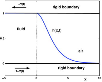
Figure 1: Schematic picture of the flow between rigid boundaries.

Using further asymptotic reductions with

$$h-1=\mathcal{O}(|V|^{-1}),\quad x=\mathcal{O}(|V|^{-1/3}),\quad t=\mathcal{O}(|V|^{-4/3}),\quad\mbox{\rm as}\quad|V|\to\infty,$$ (1.2)

the authors of [1] reduced the nonlinear equation (1.1) with $\alpha^{3}=3$ to the linear advection–diffusion equation:

$$\frac{\partial h}{\partial t}+\frac{\partial^{4}h}{\partial x^{4}}=V(t)\frac{\partial h}{\partial x},\quad x>0,\;\;t>0,$$ (1.3)

subject to the boundary conditions

$$h|_{x=0}=1,\quad h_{x}|_{x=0}=0,\quad h_{xxx}|_{x=0}=-\frac{1}{2},\quad t\geq 0,$$ (1.4)

We assume that $h,h_{x},h_{xx}\to 0$ as $x\to\infty$: in fact, any constant value of $h$ at infinity is allowed thanks to the invariance of the linear advection–diffusion equation (1.3) with respect to the shift and scaling transformations. Indeed, if $h(x,t)$ solves the boundary–value problem (1.3)–(1.4), then

$$\tilde{h}(x,t)=H+(1-H)h(\xi,\tau),\quad\xi=\frac{x}{(1-H)^{1/3}},\quad\tau=\frac{t}{(1-H)^{4/3}},$$

with constant $H<1$ solves the same advection–diffusion equation (1.3) with the same boundary conditions (1.4) but for the variable speed $\tilde{V}(t)=\frac{V(\tau)}{1-H}$ and with the asymptotic value $h(x,t)\to H$ as $x\to\infty$.

With three boundary conditions at $x=0$ and the decay conditions as $x\to\infty$, the initial-value problem for equation (1.3) is over-determined and the third (over-determining) boundary condition at $x=0$ is used to find the dependence of $V$ on $t$. Local existence of solutions to the boundary–value problem (1.3)–(1.4) was proved in our work [7] using Laplace transform in $x$ and the fractional power series expansion in $t$.

We shall consider the time evolution of the boundary–value problem (1.3)–(1.4) starting with the initial data $h|_{t=0}=h_{0}(x)$ for a suitable function $h_{0}$. In particular, we assume that the profile $h_{0}(x)$ decays monotonically to zero as $x\to\infty$ and that $0$ is a non-degenerate maximum of $h_{0}$ such that $h_{0}(0)=1$, $h_{0}^{\prime}(0)=0$, and $h_{0}^{\prime\prime}(0)<0$. If the solution $h(x,t)$ losses monotonicity in $x$ during the dynamical evolution, for instance, due to the value of

$$\beta(t):=h_{xx}(0,t)$$ (1.5)

crossing $0$ from the negative side, then we say that the flow becomes non-physical for further times and the model breaks. Simultaneously, this may mean that the velocity $V(t)$ blows up, as it is defined for sufficiently strong solutions of the advection–diffusion equation (1.3) by the pointwise equation:

$$h_{xxxxx}(0,t)=V(t)\beta(t),$$ (1.6)

which follows by differentiation of (1.3) in $x$ and setting $x\to 0$.

The main claim of [1] based on numerical computations of the reduced equation (1.3) as well as more complicated thin-film equations is that for any suitable $h_{0}$, there is a finite positive time $t_{0}$ such that $V(t)\to-\infty$ and $\beta(t)\to 0^{-}$ as $t\uparrow t_{0}$. Moreover, it is claimed that $V(t)$ behaves near the blowup time as the logarithmic function of $t$, e.g.

$$V(t)\sim C_{1}\log(t_{0}-t)+C_{2},\quad\mbox{\rm as}\quad t\uparrow t_{0},$$ (1.7)

where $C_{1}$, $C_{2}$ are positive constants.

The goal of this paper is to inspect possible blow-up rates of the singularity formation in the boundary-value problem (1.3)–(1.4). First, we use apriori energy estimates to show that $V(t)$ cannot remain positive for all times for smooth solutions of the boundary–value problem (1.3)–(1.4). This result implies simultaneously two things: if $V(t)$ remains positive, the smooth solution blows up in a finite time, and if a smooth solution exists for all times, then $V(t)$ either oscillates or become negative. Similarly, we also show that $\beta(t)$ and $V(t)\beta^{2}(t)$ cannot remain negative for all times in the same sense: if $\beta(t)$ and $V(t)\beta^{2}(t)$ remain negative, the smooth solution blows up in a finite time, and if a smooth solution exists for all times, then $\beta(t)$ and $V(t)\beta^{2}(t)$ either oscillate or become positive. Combination of both results shows that the only way a smooth solution can exist for all times is if the variable speed $V(t)$ oscillates from positive to negative values back and forth.

Second, we study the class of self-similar solutions based on the scaling transformation (1.2). The class of self-similar solutions is defined by the linear advection–diffusion equation (1.3), the decay condition at infinity, and the first two boundary conditions (1.4). The third boundary condition $h_{xxx}|_{x=0}=-\frac{1}{2}$ is not satisfied for the self-similar solutions and we replace this boundary condition with new condition $h_{xxx}|_{x=0}=\gamma_{0}V(t)$ for a fixed $\gamma_{0}<0$. We show that the solution blows up in a finite time for positive $V(t)$ and positive $\beta(t)$, which agrees with the scaling transformation (1.2) but does not correspond to the physical requirements of the flow on Figure 1.

Finally, we study how $\beta(t)$ may vanish and $V(t)$ may diverge in a finite time by using the pointwise equation (1.6) and its derivative. We find yet another rate of singularity formulations, which is different from the rates based on the scaling transformation (1.2) and on the numerically claimed result (1.7). Therefore, further studies of the boundary-value problem (1.3)–(1.4) including more precise numerical studies are required. These studies will be reported elsewhere.

The remainder of this paper is organized as follows. Section 2 gives apriori energy estimates for the boundary–value problem (1.3)–(1.4). Section 3 describes self-similar solutions describing blow-up rate of the singularity formulations. Section 4 reports analysis following from pointwise equations.

2 Apriori energy estimates

Let us consider the advection-diffusion equation (1.3) subject to the boundary conditions (1.4) and the decay condition $h,h_{x},h_{xx}\to 0$ as $x\to\infty$. We assume existence of a smooth solution to this boundary-value problem and show that $V(t)$ cannot remain positive for all times.

Theorem 1

Solutions of the boundary–value problem (1.3)–(1.4) do not exist in class $h\in C(\mathbb{R}_{+},L^{2}(\mathbb{R}_{+}))\cap L^{2}(\mathbb{R}_{+},H^{2}(\mathbb{R}_{+}))$ if $V(t)\geq V_{0}>-1$ for all $t\geq t_{0}\geq 0$.

Proof.

From the advection-diffusion equation (1.3), we have the energy balance:

$$\partial_{t}\left(\frac{1}{2}h^{2}\right)+\partial_{x}\left(hh_{xxx}-h_{x}h_{xx}-\frac{1}{2}V(t)h^{2}\right)+(h_{xx})^{2}=0.$$

Integrating this equation in $x$ on $(0,\infty)$ and using the boundary conditions (1.4) and the decay conditions as $x\to\infty$, we obtain apriori energy estimates:

$$\frac{d}{dt}\|h(\cdot,t)\|_{L^{2}(\mathbb{R}_{+})}^{2}+2\|h_{xx}(\cdot,t)\|^{2}_{L^{2}(\mathbb{R}_{+})}=-(1+V(t)).$$ (2.1)

If we have a solution in class $h\in C(\mathbb{R}_{+},L^{2}(\mathbb{R}_{+}))\cap L^{2}(\mathbb{R}_{+},H^{2}(\mathbb{R}_{+}))$, then integrating the apriori energy estimate (2.1), we obtain

$$\|h(\cdot,t)\|_{L^{2}(\mathbb{R}_{+})}^{2}+2\int_{0}^{t}\|h_{xx}(\cdot,\tau)\|^{2}_{L^{2}(\mathbb{R}_{+})}d\tau=\|h_{0}\|_{L^{2}(\mathbb{R}_{+})}^{2}-\int_{0}^{t}(1+V(\tau))d\tau.$$ (2.2)

Since the left-hand-side is strictly positive, the assertion of the theorem is proved. ∎

Next, we rewrite the advection–diffusion equation (1.3) for the variable $u=h_{x}$ in the form

$$u_{t}+u_{xxxx}=V(t)u_{x},\quad\;x>0,\;\;t>0,$$ (2.3)

subject to the boundary conditions at the contact line

$$u|_{x=0}=0,\quad u_{xx}|_{x=0}=-\frac{1}{2},\quad u_{xxx}|_{x=0}=0,\quad t\geq 0,$$ (2.4)

where the boundary conditions $u_{xxx}|_{x=0}=h_{xxxx}|_{x=0}=0$ follows from the boundary conditions $h|_{x=0}=1$ and $h_{x}|_{x=0}=0$ as well as the advection–diffusion equation (1.3) as $x\to 0$. Denote $\beta(t)=h_{xx}|_{x=0}=u_{x}|_{x=0}$ and recall that $\beta(0)<0$ initially. Again, we assume existence of a smooth solution to the boundary-value problem (2.3)–(2.4) and show that $\beta(t)$ and $V(t)\beta^{2}(t)$ cannot remain negative for all times.

Theorem 2

Solutions of the boundary–value problem (2.3)–(2.4) do not exist in class $u\in C(\mathbb{R}_{+},L^{2}(\mathbb{R}_{+}))\cap L^{2}(\mathbb{R}_{+},H^{2}(\mathbb{R}_{+}))$ if $\beta(t)\leq\beta_{0}<0$ for all $t\geq t_{0}\geq 0$.

Proof.

From the advection-diffusion equation (2.3), we have the energy balance:

$$\partial_{t}\left(\frac{1}{2}u^{2}\right)+\partial_{x}\left(uu_{xxx}-u_{x}u_{xx}-\frac{1}{2}V(t)u^{2}\right)+(u_{xx})^{2}=0.$$

Integrating this equation in $x$ on $(0,\infty)$ and using the boundary conditions (2.4) and the decay conditions as $x\to\infty$, we obtain apriori energy estimates:

$$\frac{d}{dt}\|u(\cdot,t)\|_{L^{2}(\mathbb{R}_{+})}^{2}+2\|u_{xx}(\cdot,t)\|^{2}_{L^{2}(\mathbb{R}_{+})}=\beta(t).$$ (2.5)

If we have a solution in class $u\in C(\mathbb{R}_{+},L^{2}(\mathbb{R}_{+}))\cap L^{2}(\mathbb{R}_{+},H^{2}(\mathbb{R}_{+}))$, then integrating the apriori energy estimate (2.5), we obtain

$$\|u(\cdot,t)\|_{L^{2}(\mathbb{R}_{+})}^{2}+2\int_{0}^{t}\|u_{xx}(\cdot,\tau)\|^{2}_{L^{2}(\mathbb{R}_{+})}d\tau=\|u_{0}\|_{L^{2}(\mathbb{R}_{+})}^{2}+\int_{0}^{t}\beta(\tau)d\tau.$$ (2.6)

Since the left-hand-side is strictly positive, the assertion of the theorem follows. ∎

Theorem 3

Solutions of the boundary–value problem (2.3)–(2.4) do not exist in class $u\in C(\mathbb{R}_{+},H^{1}(\mathbb{R}_{+}))\cap L^{2}(\mathbb{R}_{+},H^{3}(\mathbb{R}_{+}))$ if $V(t)\leq V_{0}<0$ and $|\beta(t)|\geq\beta_{0}>0$ for all $t\geq t_{0}\geq 0$.

Proof.

Multiplying the advection-diffusion equation (2.3) by $u_{xx}$, integrating this equation in $x$ on $(0,\infty)$, and using the boundary conditions (2.4) and the decay conditions as $x\to\infty$, we obtain apriori energy estimates:

$$\frac{d}{dt}\|u_{x}(\cdot,t)\|_{L^{2}(\mathbb{R}_{+})}^{2}+2\|u_{xxx}(\cdot,t)\|^{2}_{L^{2}(\mathbb{R}_{+})}=V(t)\beta^{2}(t).$$ (2.7)

If we have a solution in class $u\in C(\mathbb{R}_{+},H^{1}(\mathbb{R}_{+}))\cap L^{2}(\mathbb{R}_{+},H^{3}(\mathbb{R}_{+}))$, then integrating the apriori energy estimate (2.7), we obtain

$$\|u_{x}(\cdot,t)\|_{L^{2}(\mathbb{R}_{+})}^{2}+2\int_{0}^{t}\|u_{xxx}(\cdot,\tau)\|^{2}_{L^{2}(\mathbb{R}_{+})}d\tau=\|u_{0}^{\prime}\|_{L^{2}(\mathbb{R}_{+})}^{2}+\int_{0}^{t}V(\tau)\beta^{2}(\tau)d\tau.$$ (2.8)

Since the left-hand-side is strictly positive, the assertion of the theorem follows. ∎

3 Self-similar solutions for singularity formations

Let us consider the class of self-similar solutions to the linear advection–diffusion equation (1.3):

$$V(t)=\frac{t_{0}V_{0}}{(t_{0}-t)^{3/4}},\quad h(x,t)=f(\xi),\quad\xi=\frac{x}{(t_{0}-t)^{1/4}},$$ (3.1)

where $t_{0}$ is an arbitrary positive parameter for a finite blowup time, $V_{0}$ is an arbitrary parameter for the initial velocity, and $f(\xi)$ is a solution of the differential equation:

$$\frac{d^{4}f}{d\xi^{4}}+\frac{1}{4}(\xi-4t_{0}V_{0})\frac{df}{d\xi}=0,\quad\xi>0.$$ (3.2)

We are looking at a solution of the boundary-value problem associated with the first two boundary conditions at the contact line:

$$f(0)=1,\quad f^{\prime}(0)=0,$$ (3.3)

and the decay condition $f(\xi),f^{\prime}(\xi)\to 0$ as $\xi\to\infty$. Note that the third condition at the contact line $h_{xxx}|_{x=0}=-\frac{1}{2}$ is not satisfied by the self-similar solution (3.1). The revised third boundary condition is given by

$$h_{xxx}|_{x=0}=\frac{f^{\prime\prime\prime}(0)}{(t_{0}-t)^{3/4}}=\gamma_{0}V(t),$$ (3.4)

where $\gamma_{0}$ is constant such that $f^{\prime\prime\prime}(0)=t_{0}V_{0}\gamma_{0}$. Also note that the class of self-similar solutions (3.1) is compatible with the asymptotic scaling (1.2) used in the derivation of the linear advection-diffusion equation (1.3).

Setting

$$g(z)=f^{\prime}(\xi),\quad z=\xi-4t_{0}V_{0},$$

we reduce the boundary-value problem (3.2)–(3.3) to the following system:

$$\left\{\begin{array}[]{l}4g^{\prime\prime\prime}(z)+zg(z)=0,\quad\quad z>z_{0},\\ g(z_{0})=0,\\ g(z),g^{\prime}(z)\to 0\quad\mbox{\rm as}\;\;z\to\infty,\end{array}\right.$$ (3.5)

where $z_{0}=-4t_{0}V_{0}$. A suitable solution of this boundary–value problem is constructed in the following theorem.

Theorem 4

There exists a unique (up to scalar multiplication) positive solution of the boundary–value problem (3.5) on $(z_{0},\infty)$ with $z_{0}<0$.

Proof.

As $z\to\infty$, there are three fundamental solutions of the linear equation

$$4g^{\prime\prime\prime}(z)+zg(z)=0.$$ (3.6)

One solution decays to $0$ monotonically as $z\to\infty$ and the other two solutions oscillate and diverge as $z\to\infty$. Therefore, the space of solutions of the boundary–value problem (3.5) is spanned by a particular solution (denoted by $G$) decaying to $0$ at infinity. To define $G$ uniquely, we construct a decaying solution of the differential equation (3.6) asymptotically by using the WKB analysis [5]:

$$G(z)=\exp\left(-\frac{3z^{4/3}}{2^{8/3}}\right)\left[\frac{1}{z^{1/3}}+\mathcal{O}\left(\frac{1}{z^{2/3}}\right)\right]\quad\mbox{\rm as}\quad z\to\infty,$$ (3.7)

where corrections terms can be identified in terms of power series in inverse powers of $z^{1/3}$. The solution $G$ of the linear equation (3.6) can be extended globally for all $z\in\mathbb{R}$. To satisfy the boundary condition at $z_{0}$, it remains to show that there is $z_{0}\in\mathbb{R}$ such that $G(z_{0})=0$.

It is clear that $z_{0}\in\mathbb{R}$ exists. Indeed, if $z_{0}$ does not exist, then $G(z)$ remains positive for all $z\in\mathbb{R}$, which is only possible if $G(z)$ decays to $0$ monotonically as $z\to-\infty$ (the other two solutions again oscillate and diverge as $z\to-\infty$). However, then $G\in H^{2}(\mathbb{R})$ is a global solution of the differential equation (3.6) for all $z\in\mathbb{R}$. Multiplying this equation by $G^{\prime}$ and integrating by parts, we obtain the contradiction

$$4\int_{\mathbb{R}}(G^{\prime\prime})^{2}dz+\frac{1}{2}\int_{\mathbb{R}}G^{2}dz=0,$$ (3.8)

which proves that no $G\in H^{2}(\mathbb{R})$ may exist. Furthermore, $z_{0}<0$ because $G(z)$ is monotonically decaying for all $z>0$. To see this, we use the fact that the differential equation (3.6) is invariant under the transformation $z\mapsto-z$, so that $\tilde{G}(z):=G(-z)$ is another solution of (3.6). The function $\tilde{G}(z)$ increases monotonically for large negative $z$. Since $4\tilde{G}^{\prime\prime\prime}(z)=-z\tilde{G}(z)>0$ for all $z<0$, $\tilde{G}(z)$ remains monotonically increasing for all $z\leq 0$ and hence $G(z)$ decreases monotonically for all $z\geq 0$. Therefore, $z_{0}<0$, that is, $V_{0}>0$ (if $t_{0}>0$). The value $z_{0}$ is uniquely determined as the largest negative zero of the positive function $G(z)$. ∎

Figure 2 shows numerical approximation of the solution $G(z)$ satisfying the boundary–value problem (3.2). The numerical approximation is obtained with the standard Heun method.

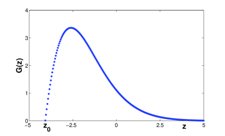
Figure 2: Numerical approximation of the solution $G(z)$ of the boundary–value problem (3.2).

A general solution of the boundary-value problem (3.5) is given by $g(z)=CG(z)$. To determine the constant $C$, we use the modified boundary condition (3.4). If $h_{xxx}|_{t=0}<0$ as inherited from the third boundary condition in (1.4), we should have $g^{\prime\prime}(0)=f^{\prime\prime\prime}(0)<0$ or $CG^{\prime\prime}(z_{0})<0$. By the continuity arguments, we have $G^{\prime\prime}(z_{0})<0$ and therefore, $C>0$. Indeed, $\tilde{G}(z):=G(-z)$ is monotonically increasing function for all $z\leq 0$ with $4\tilde{G}^{\prime\prime\prime}(z)=-z\tilde{G}(z)>0$. When $z>0$, $\tilde{G}^{\prime\prime\prime}(z)<0$ as long as $\tilde{G}(z)>0$, so that there is $\tilde{z}_{0}\in(0,z_{0})$, such that $\tilde{G}^{\prime\prime}(z)<0$ for all $z\in(-\tilde{z}_{0},-z_{0}]$, or equivalently, $G^{\prime\prime}(z)<0$ for all $z\in[z_{0},\tilde{z}_{0})$. Therefore, $G^{\prime\prime}(z_{0})<0$ as on Figure 2.

By the same argument, there is $\tilde{\tilde{z}}_{0}\in(\tilde{z}_{0},z_{0}]$ such that $\tilde{G}^{\prime}(z)<0$ for all $z\in(-\tilde{\tilde{z}}_{0},-z_{0}]$, or equivalently, $G^{\prime}(z)>0$ for all $z\in[z_{0},\tilde{\tilde{z}}_{0})$. Therefore, $G^{\prime}(z_{0})>0$ as on Figure 2, which implies that

$$\beta(t)=\frac{f^{\prime\prime}(0)}{(t_{0}-t)^{1/2}}=\frac{CG^{\prime}(z_{0})}{(t_{0}-t)^{1/2}}>0,\quad t\in[0,t_{0}).$$

We conclude that the class of self-similar solutions (3.1) does not represent the relevant dynamics of the boundary-value problem (1.3)–(1.4) in the context of the physical requirements of the flow on Figure 1 because $\beta(t)$ is supposed to be negative at least for initial values of $t\geq 0$.

4 Pointwise equations

We give here additional estimates of how the solution of the boundary–value problem (1.3)–(1.4) may blow up in a finite time, based on the pointwise equation (1.6) and its derivative. We look at the boundary–value problem (2.3)–(2.4) and assume existence of a sufficiently smooth solution. By taking the limit $x\to 0$, we recover the pointwise equation (1.6) rewritten in new variables as

$$u_{xxxx}|_{x=0}=V(t)\beta(t),\quad t\geq 0,$$ (4.1)

where $\beta(t)=u_{x}|_{x=0}$. By taking a derivative of the linear advection–diffusion equation (2.3) in $x$ and the limit $x\to 0$, we obtain another pointwise equation:

$$\frac{d\beta}{dt}+u_{xxxxx}|_{x=0}=-\frac{1}{2}V(t),\quad t\geq 0.$$ (4.2)

The system of equations (4.1) and (4.2) can be rewritten in the partially closed form:

$$\frac{d\beta}{dt}=-\frac{u_{xxxx}|_{x=0}}{2\beta(t)}-u_{xxxxx}|_{x=0},\quad t\geq 0.$$ (4.3)

Let us now assume that there is $t_{0}>0$ such that

$$\beta(t)\to 0,\quad u_{xxxx}|_{x=0}\to a_{4},\quad u_{xxxxx}|_{x=0}\to a_{5},\quad\mbox{\rm as}\quad t\uparrow t_{0},$$ (4.4)

where $a_{4}\neq 0$ and $|a_{5}|<\infty$. Then, asymptotic analysis of the differential equation (4.3) shows that

$$\beta^{2}(t)=a_{4}(t_{0}-t)+\mathcal{O}(t_{0}-t)^{3/2},\quad V(t)=\sqrt{\frac{a_{4}}{t_{0}-t}}+\mathcal{O}(1),\quad\mbox{\rm as}\quad t\uparrow t_{0},$$ (4.5)

under the constraint that $a_{4}>0$. The asymptotic rate (4.5) is different both from the scaling transformation (1.2) and the numerically claimed result (1.7). In the context of the numerical result (1.7), this pointwise analysis may imply that either $a_{4}=0$ or $a_{5}\to\infty$ in the assumption (4.4).

We conclude that three different rates of the singularity formations claimed in (1.7) and obtained in (3.1) and (4.5) indicate complexity of dynamics of the boundary-value problem (1.3)–(1.4) or its equivalent version (2.3)–(2.4). Further studies of dynamical evolution of contact lines within this reduced problem are needed, including more precise numerical simulations.

Acknowledgement: The authors are thankful to E.S. Benilov and R. Taranets for useful discussions and for sharing their unpublished results at an early stage of his research.

References

- [1] E.S. Benilov and M. Vynnycky, “Contact lines with a contact angle”, submitted to J. Fluid Mech. (2012)
- [2] D.J. Benney and W.J. Timson, “The rolling motion of a viscous fluid on and off a rigid surface”, Stud. Appl. Math. 63 (1980), 93–98.
- [3] M. Chugunova, M. Pugh, and R. Taranets, “Nonnegative solutions for a long-wave unstable thin film equation with convection”, SIAM J. Math. Anal. 42, 1826-1853 (2010).
- [4] M. Chugunova and R. Taranets, “Qualitative analysis of coating flows on a rotating horizontal cylinder”, Int. J. Diff. Eqs. 2012 (2012), Article ID 570283, 30 pages.
- [5] J.A. Murdock, Perturbations: Theory and Methods (SIAM, Philadelphia, 1987).
- [6] C.G. Ngan and V.E.B. Dussan, “The moving contact line with a advancing contact angle”, Phys. Fluids 24 (1984), 2785–2787.
- [7] D.E. Pelinovsky, A.R. Giniyatullin, and Y.A. Panfilova, “On solutions of a reduced model for the dynamical evolution of contact lines”, submitted (2012).