Quantum Excitations in Time-Dependent Backgrounds

Abstract

We give a technique for calculating the occupation number of quantum fields in time-dependent backgrounds by using the relation between one-dimensional quantum oscillators and two-dimensional classical oscillators. We illustrate our method by giving closed analytical results for the time-dependent spectrum of occupation numbers during gravitational collapse in any number of dimensions.

Frequently we are interested in calculating the spectrum of excitations of a quantum field produced due to a time-dependent background. The context can range from nuclear physics, condensed matter systems, gravitational systems, and cosmology, and includes particle production during gravitational collapse or in an expanding universe. Usually such problems are solved by the method of Bogoliubov transformations Bogoliubov:1947 ; BirrellDavies , and require knowledge of all the modes of the quantum field at the initial and final times. Then the excitation spectrum, as well as local information, e.g. energy-momentum densities, can be obtained. However, in certain cases it may be difficult to find all the modes of the quantum field, especially in a time-dependent situation, and it is desirable to find a short cut to the spectrum of excitations, even if all the detailed local information is not available. In this paper, we propose such a method based on the functional Schrodinger equation that can be applied to certain systems. We illustrate the method in the special case of quantum excitations produced during gravitational collapse.

Consider a scalar field $\Phi(t,{\bf x})$ that is free but for interaction with a time-dependent background e.g. a time-varying mass parameter or background metric. We can always expand the field in a complete basis of functions,

$$\Phi(t,{\bf x})=\sum_{k}a_{k}(t)f_{k}({\bf x})$$ (1)

where $k$ denotes a complete set of mode numbers. The $f_{k}$’s need not be a set of (instantaneous) mode functions; the only requirement is that any function of ${\bf x}$ should be expressible as a linear sum of $f_{k}$’s. On inserting this form in the action, we obtain

$$S=\int dt\left[\frac{1}{2}{\dot{a}}_{k}\bar{\bf M}_{kl}(t){\dot{a}}_{l}-\frac{1}{2}a_{k}{\bf V}_{kl}(t)a_{l}\right]$$ (2)

where $\bar{\bf M}$ and ${\bf V}$ are real, symmetric matrices that are given by spatial integrals over products of the basis functions and their derivatives. They depend on time due to the interaction of $\Phi$ and the background, and a sum over repeated indices in Eq. (2) is implicit. In general, the elements of $\bar{\bf M}$ will have complicated time dependence and the problem appears intractable. However, progress can be made if the time dependence can be pulled out,

$$\bar{\bf M}=\frac{1}{B(t)}{\bf M}$$ (3)

where ${\bf M}$ is independent of time. Such a simplification occurs for gravitational collapse because $B\to 0$ and then ${\bar{\bf M}}$ has the form in Eq. (3) to leading order in $1/B$ Vachaspati:2006ki . Similar simplification will also occur in cosmological spacetimes in which all the time dependence is in an overall scale factor.

With Eq. (3) one can write,

$$S=\int d\eta\left[\frac{1}{2}a_{k}^{\prime}{\bf M}_{kl}a_{l}^{\prime}-\frac{1}{2B(\eta)}a_{k}{\bf V}_{kl}(\eta)a_{l}\right]$$ (4)

where primes denote derivatives with respect to a new time coordinate $\eta$ that is defined by

$$\frac{d\eta}{dt}=B(t)$$ (5)

Now we attempt to do a “principal axis transformation”. As is standard procedure Goldstein , first we diagonalize ${\bf M}$. Then by a rescaling transformation, ${\bf M}$ can be transformed into the identity matrix. Since ${\bf M}$ is taken to be independent of time, the diagonalization and rescaling transformations are time independent.. The transformed potential matrix will still be time dependent. The tractable case is when the transformed potential matrix can be diagonalized by a time independent transformation. The final action takes the form

$$S=\sum_{k}\int d\eta\left[\frac{1}{2}{b_{k}^{\prime}}^{2}-\frac{v_{k}(\eta)}{2B(\eta)}b_{k}^{2}\right]$$ (6)

where $b_{k}$’s are the transformed mode coefficients and $v_{k}(\eta)$ are the eigenvalues of the transformed potential matrix. It should be noted that the principal axis transformation can be implemented even if the matrices ${\bf M}$ and ${\bf V}$ do not commute. The theorem that only commuting matrices can be simultaneously diagonalized applies when we restrict the diagonalization procedure to similarity transformations. The principle axis transformation involves a rescaling which is not implemented by a similarity transformation.

We can now quantize each mode separately. The Schrodinger equation for a mode is

$$\biggl{[}-\frac{1}{2}\frac{\partial^{2}}{\partial b^{2}}+\frac{1}{2}\omega^{2}(\eta)b^{2}\biggr{]}\psi(b,\eta)=i\frac{\partial}{\partial\eta}\psi(b,\eta)$$ (7)

where we have omitted the mode label $k$ for convenience and written the equation in a form reminiscent of the simple harmonic oscillator (SHO). The only time dependence is due to a time varying frequency $\omega(\eta)$.

The Schrodinger equation has the “ground state” solution Dantas:1990rk

$$\psi(b,\eta)=e^{i\alpha(\eta)}\left(\frac{1}{\pi\rho^{2}}\right)^{1/4}\exp\left[\frac{i}{2}\left(\frac{\rho_{\eta}}{\rho}+\frac{i}{\rho^{2}}\right)b^{2}\right]$$ (8)

where $\rho_{\eta}$ denotes derivative of $\rho(\eta)$ with respect to $\eta$, and $\rho$ is given by the real solution of the ordinary differential equation

$${\rho_{\eta\eta}}+\omega^{2}(\eta)\rho=\frac{1}{\rho^{3}}.$$ (9)

Initial conditions for $\rho$ are chosen so that the wave function yields the ground state of the time-independent SHO at $\eta=0$,

$$\rho(0)=\frac{1}{\sqrt{\omega_{0}}}\ ,\ \ \ {\rho_{\eta}}(0)=0$$ (10)

where $\omega_{0}\equiv\omega(0)$. The phase $\alpha$ is given by

$$\alpha(\eta)=-\frac{1}{2}\int_{0}^{\eta}\frac{d\eta^{\prime}}{\rho^{2}(\eta^{\prime})}$$ (11)

The wave function in Eq. (8) can now be expanded in the “instantaneous” SHO eigenfunctions with frequency $\omega(\eta)$. The occupation number of the mode is given by the expectation value of the quantum number of the excitation. The occupation number as a function of time and frequency can be written as Vachaspati:2006ki

$$N(t,\omega_{0})=\frac{1}{4{\omega}\rho^{2}}\left[({\omega}\rho^{2}-1)^{2}+(\rho\rho_{\eta})^{2}\right]$$ (12)

where the $\omega$ on the right-hand side refers to $\omega(\eta)$. In (12) we have corrected the pre-factor stated in Ref. Vachaspati:2006ki , $1/4$ instead of $1/\sqrt{2}$ .

The crucial step that remains is to solve Eq. (9) and it is here that the remarkable connection between quantum SHO in 1 dimension and classical SHO in 2 dimensions comes into play Lewis:1968 ; Lewis:1969 ; Brown:1991zz ; Song:2000 ; Parker:1971 . The solution for $\rho$ is given by the solutions for two classical SHO’s $\xi$ and $\chi$, each of which satisfies the equation

$$f_{\eta\eta}+\omega^{2}(\eta)f=0.$$ (13)

Then the solution for $\rho$ is

$$\rho=\frac{1}{\sqrt{\omega_{0}}}\sqrt{\xi^{2}+\chi^{2}}.$$ (14)

The initial conditions for $\rho$ can be satisfied provided

$$\xi(0)=1,\ \ \xi_{\eta}(0)=0,\ \ \chi(0)=0,\ \ \chi_{\eta}(0)=\omega_{0}$$ (15)

The time derivative of $\rho$, which occurs in the wave function, can be written in terms of $\xi$ and $\chi$ and their derivatives,

$$\rho_{\eta}=\frac{1}{\omega_{0}\rho}(\xi\xi_{\eta}+\chi\chi_{\eta}).$$ (16)

An explicit scheme for constructing solutions with the correct initial conditions can now be described. We start with the classical SHO equation (13) and let $f_{1}$ and $f_{2}$ be any linearly independent solutions. Then the solutions with the correct initial conditions in Eq. (15) are given by

$$\xi(\omega_{0},\eta)=W^{-1}(f_{2\eta}(\omega_{0},\eta_{i})f_{1}(\omega_{0},\eta)-f_{1\eta}(\omega_{0},\eta_{i})f_{2}(\omega_{0},\eta))$$ (17)

$$\chi(\omega_{0},\eta)=-\omega_{0}W^{-1}(f_{2}(\omega_{0},\eta_{i})f_{1}(\omega_{0},\eta)-f_{1}(\omega_{0},\eta_{i})f_{2}(\omega_{0},\eta))$$ (18)

$$\xi_{\eta}(\omega_{0},\eta)=W^{-1}(f_{2\eta}(\omega_{0},\eta_{i})f_{1\eta}(\omega_{0},\eta)-f_{1\eta}(\omega_{0},\eta_{i})f_{2\eta}(\omega_{0},\eta))$$ (19)

$$\chi_{\eta}(\omega_{0},\eta)=-\omega_{0}W^{-1}(f_{2}(\omega_{0},\eta_{i})f_{1\eta}(\omega_{0},\eta)-f_{1}(\omega_{0},\eta_{i})f_{2\eta}(\omega_{0},\eta))$$ (20)

where $\omega_{0}\equiv\omega(0)$ and $W$ is the Wronskian defined as

$$W=f_{2\eta}(\omega_{0},\eta_{i})f_{1}(\omega_{0},\eta_{i})-f_{1\eta}(\omega_{0},\eta_{i})f_{2}(\omega_{0},\eta_{i})$$ (21)

Now it is simply a matter of finding $\rho$ and $\rho_{\eta}$ from equations (14) and (16), and then inserting into the occupation number formula (12).

We will illustrate the above method by applying it to particle production of a massless scalar field during gravitational collapse of a spherical domain wall in 3 spatial dimensions. The function $B(t)$ in Eq. (3) is given by Vachaspati:2006ki

$$B(t)=1-\frac{R_{S}}{R(t)}$$ (22)

where $R(t)$ is the radius of the wall at time $t$, and $R_{S}$ is the Schwarzschild radius. For convenience we will set $R_{S}=1$. Using the classical solution for $R(t)$ in the late time limit and Eq. (5), a model for $\omega(\eta)$ can be taken to be

$$\omega(\eta)=\frac{\omega_{0}}{\sqrt{B(\eta)}}=\frac{\omega_{0}}{\sqrt{1-\eta}}$$ (23)

Then (13) can be solved in terms of Bessel functions e.g. see aands . With the help of Eqs. (17-20), we get

$$\xi=\frac{\pi u}{2}[Y_{0}(2\omega_{0})J_{1}(u)-J_{0}(2\omega_{0})Y_{1}(u)]$$ (24)

$$\chi=\frac{\pi u}{2}[Y_{1}(2\omega_{0})J_{1}(u)-J_{1}(2\omega_{0})Y_{1}(u)]$$ (25)

$$\xi_{\eta}=-\pi\omega_{0}^{2}[Y_{0}(2\omega_{0})J_{0}(u)-J_{0}(2\omega_{0})Y_{0}(u)]$$ (26)

$$\chi_{\eta}=-\pi\omega_{0}^{2}[Y_{1}(2\omega_{0})J_{0}(u)-J_{1}(2\omega_{0})Y_{0}(u)]$$ (27)

where $u\equiv 2\omega_{0}\sqrt{1-\eta}$. The particle occupation number per mode at time $t$ and frequency $\omega_{0}$ is found from Eq. (12) and can be written as Vachaspati:2006ki

$$N(t,\omega_{0})=\frac{\sqrt{1-\eta}}{4(\xi^{2}+\chi^{2})}\left[\left(\frac{\xi^{2}+\chi^{2}}{\sqrt{1-\eta}}-1\right)^{2}+\frac{1}{\omega_{0}^{2}}(\xi\xi_{\eta}+\chi\chi_{\eta})^{2}\right].$$ (28)

where $\xi$, $\chi$, $\xi_{\eta}$, $\chi_{\eta}$ are given in Eqs. (24), (25), (26), and (27).

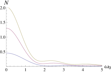
Figure 1: Occupation number, $N$, as a function of $\omega_{0}$ for $\eta=0.92$, $0.98$, and $0.99$ (lowest to highest curve).

In Fig. 1 we plot the spectrum of occupation numbers at three different times. The plot can also be made in terms of $\Omega$, the final frequency corresponding to the original time parameter $t$; $\Omega$ is also the frequency relevant for an asymptotic observer. The relation between $t$ and $\eta$ is obtained from Eq. (5),

$$t=\int\frac{d\eta}{B(\eta)}=\int\frac{d\eta}{1-\eta}=-\ln(1-\eta).$$ (29)

and the relation between $\Omega$ and $\omega_{0}$ is

$$\Omega=\frac{d\eta}{dt}\omega(\eta)=e^{-t/2}\omega_{0}.$$ (30)

The occupation number spectrum in terms of $\Omega$ is shown in Fig. 2, and Fig. 3 illustrates the time dependence of the occupation number at three different frequencies.

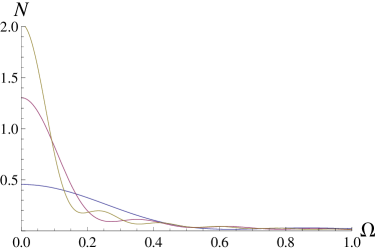
Figure 2: Occupation number, $N$, as a function of $\Omega$ for $\eta=0.92$, $0.98$, and $0.99$ (lowest to highest curve at origin).

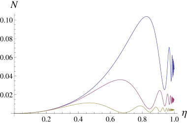
Figure 3: Occupation number versus $\eta$ for $\Omega=0.5$, $1$, and $2$ (highest to lowest curve).

Limiting forms of the occupation numbers in different frequency ranges are obtained by using expansions of the Bessel functions. The final results can be written as

$$N\approx\begin{cases}{e^{t/2}}/4,\ \ \ \ &2\Omega\ll e^{-t/2}\\ {1}/(4\pi\Omega),\ \ \ \ &e^{-t/2}\ll 2\Omega\ll 1\\ {1}/(64\Omega^{2}),\ \ \ \ &1\ll 2\Omega.\end{cases}$$ (31)

It is also possible to give a closed formula for the occupation numbers for $t\to\infty$ that is valid at all frequencies

$$N\to\frac{1}{4}\frac{\pi\Omega}{(J_{1}^{2}+Y_{1}^{2})}\left[\biggl{\{}J_{1}^{2}+Y_{1}^{2}-\frac{1}{\pi\Omega}\biggr{\}}^{2}+\biggl{\{}J_{0}J_{1}+Y_{0}Y_{1}\biggr{\}}^{2}\right]$$ (32)

where all the Bessel functions have argument $2\Omega$.

The occupation number in the intermediate regime $e^{-t/2}=\sqrt{1-\eta}\ll 2\Omega\ll 1$ correspond to the low frequency part of the thermal blackbody temperature

$$N_{\rm T}=\frac{1}{e^{\Omega/T}-1}$$ (33)

if we take the temperature to be

$$T=\frac{1}{4\pi}$$ (34)

in units where the Schwarzschild radius $R_{S}=1$. This temperature is precisely the Hawking temperature Hawking:1974sw . The very low frequency limit in Eq. (31) only coincides with the divergent thermal value if we take $\eta\to 1$ ($t\to\infty$).

The high frequency limit in Eq. (31) does not match the exponentially (Boltzmann) suppressed thermal expression. This can be understood by noting that our calculation yields occupation numbers during the collapse and includes all excitations that are produced, including transients and non-radiative excitations (vacuum polarization). Such non-thermal features are also seen in a treatment of gravitational collapse in a 1+1 dimensional model Davies:1976ei ; Davies:1976 and are separated out by using the explicit mode functions to calculate the energy flux at spatial infinity . Only the radiative part, i.e. the Hawking radiation, is thermal and hence exponentially suppressed at high frequencies. If we are interested in asymptotic signatures of gravitational collapse, it is indeed only the radiative excitations that are of interest. However, if we are interested in the dynamics of the collapse, then it is necessary to consider all modes of the scalar field and the full wave function as given in Eq. (8).

The above comments highlight the advantages and limitations of the technique developed in this paper. For systems in any number of dimensions that have the simplifying properties discussed around Eqs. (3) and (6) we can obtain the complete wave function for the mode coefficients. The solution for the wave function, Eq. (8), completely characterizes the system and allows us to calculate the occupation numbers analytically and in closed form, even without explicit knowledge of the mode functions. However, it becomes necessary to find the mode functions if one requires spatial information about the excitations that are produced. Additionally, we have neglected backreaction of the radiation on the collapse. This is a difficult problem that has not seen any clear resolution in the literature; some attempts in the present formalism that lead to a modification of the wave function describing gravitational collapse may be found in Vachaspati:2007hr ; Vachaspati:2007ur .

- (1) N. Bogoliubov, J. Phys. (USSR) 11, 23 (1947).
- (2) “Quantum Fields in Curved Space”, N. Birrell and P.C.W. Davies, Cambridge University Press (1994).
- (3) “Classical Mechanics”, H. Goldstein, Addison-Wesley (1980).
- (4) C. M. A. Dantas, I. A. Pedrosa and B. Baseia, Phys. Rev. A 45, 1320 (1992).
- (5) T. Vachaspati, D. Stojkovic and L. M. Krauss, Phys. Rev. D 76, 024005 (2007) [gr-qc/0609024].
- (6) H.R. Lewis, Jr, J. Math. Phys. 9, 1976 (1968).
- (7) H.R. Lewis, Jr. and W.B. Riesenfeld, J. Math. Phys. 10, 1458 (1969).
- (8) L. S. Brown, Phys. Rev. Lett. 66, 527 (1991).
- (9) D-Y. Song, Phys. Rev. A 62, 014103 (2000).
- (10) L. Parker, Am. J. Phys. 39, 24 (1971).
- (11) “Handbook of Mathematical Functions”, M. Abramowitz and I. A. Stegun, National Bureau of Standards, Applied Mathematics Series - 55, Washington D. C. (1972); http://people.math.sfu.ca/ cbm/aands/
- (12) S. W. Hawking, Commun. Math. Phys. 43, 199 (1975) [Erratum-ibid. 46, 206 (1976)].
- (13) P. C. W. Davies, S. A. Fulling and W. G. Unruh, Phys. Rev. D 13, 2720 (1976).
- (14) P. C. W. Davies, Proc. R. Soc. Lond. A 351, 129 (1976).
- (15) T. Vachaspati and D. Stojkovic, Phys. Lett. B 663, 107 (2008) [gr-qc/0701096].
- (16) T. Vachaspati, Class. Quant. Grav. 26, 215007 (2009) [arXiv:0711.0006 [gr-qc]].