Lévy flights and nonlocal quantum dynamics

Abstract

We develop a fully fledged theory of quantum dynamical patterns of behavior that are nonlocally induced. To this end we generalize the standard Laplacian-based framework of the Schrödinger picture quantum evolution to that employing nonlocal (pseudodifferential) operators. Special attention is paid to the Salpeter (here, $m\geq 0$) quasirelativistic equation and the evolution of various wave packets, in particular to their radial expansion in 3D. Foldy’s synthesis of ”covariant particle equations” is extended to encompass free Maxwell theory, which however is devoid of any ”particle” content. Links with the photon wave mechanics are explored.

I Introduction

The standard unitary quantum dynamics and the Schrödinger semigroup-driven random motion, risken ; albeverio , are examples of dual evolution scenarios that may be mapped among each other by means of a suitable analytic continuation in time procedure. This is an offspring gar0 ; guerra ; guerra1 of Euclidean quantum field theory methods, albeit reduced to the purely quantum mechanical level. Both evolutions are generated by means of a common local Hamiltonian operator. Our departure point for subsequent analysis is an observation that a complete spectral resolution of the corresponding Hamiltonian actually determines a classical space-time homogeneous diffusion-type Markov process in $R^{n}$.

Within the general theory of so called infnitely divisible probability laws (see below) the familiar Laplacian (Wiener noise or Brownian motion generator) is known to be one isolated member of a surprisingly rich family of non-Gaussian Lévy noise generators. All of them stem from the fundamental Lévy-Khintchine formula, and typically refer to probability distributions of spatial jumps and the resultant jump-type Markov processes. That needs to be contrasted with the traditional diffusion imagery (Wiener noise and process) associated with the Laplacian, nelson .

The emergent Lévy generators are manifestly nonlocal (pseudo-differential) operators and, while being additively perturbed by a suitable external potential, give rise (via a canonical quantization procedure described subsequently) to Lévy-Schrödinger semigroups. The dual image of such semigroups comprises unitary dynamics scenarios which can be viewed as signatures of a nonlocal quantum behavior. As we discuss in below this dynamical nonlocality extends to the very concept of photons, within so-called photon wave mechanics, ibb .

Quite apart from ”Euclidean” vs ”real” time connotations, the considered dual dynamical systems refer to real time labels and clocks. Both of them drive probability density functions (pdfs) which, in the course of time evolution ($t\in R_{+}$) either maintain or develop asymptotic heavy-tails and typically have a finite number of moments in existence. This needs to be contrasted with the Gaussian standards of thinking (all pdf moments in existence, rapid decay at infinities etc.) that pervade the Laplacian-based quantum theory.

The major goal of the present paper is to set on solid grounds the quantization programme that completely avoids a reference to classical mechanics (of massive particles), normally viewed as a conceptual support for the specific choice of the Hamiltonian operator within the traditional Schrödinger wave mechanics. Here we consider a standard form of the Hamiltonian (minus Laplacian plus a perturbing potential) as an exception rather than a universally valid feature of an admissible quantum theory.

The latter is introduced by means of the most primitive quantization ansatz, whose core lies in choosing the Hilbert space $L^{2}(R^{n})$ as an arena for our investigations. From the start we have the Fourier transformation realized as a unitary operation in this space and a canonical quantization input as a straightforward consequence.

The above mentioned Lévy-Khintchine formula, while being tailored to our purposes, derives through a Fourier transform of a symmetric probability density function. A variety of symmetric probability laws for random noise is classified by means of a characteristic function which is an exponent $\eta(p)$ of the $(2\pi)^{n/2}$-multiplied Fourier transform of that pdf: $\int d^{n}x\rho(x)\exp(\pm ipx)=\exp[\eta(p)]$.

The most straightforward, naive canonical quantization step $p\rightarrow\hat{p}=-i\nabla$ (hereby limited to the symmetric pdf case) introduces the notion of random transport that is driven by Lévy-Schrödinger semigroups $\exp[t\eta(\hat{p})]$. Their dual partners actually are the unitary evolution operators $\exp[it\eta(\hat{p})]$ of interest and are a subject of further discussion.

In the present paper we develop a complete theory that starts from diffusion type processes and their semigroup reconstruction, followed by the duality mapping. Next we pass to general jump-type stochastic processes that stem from the Lévy-Khintchine formula and pass to the dual (e.g. quantum) dynamics, with a number of specific physically motivated examples, like the Salpeter Hamiltonian and its $m=0$ Cauchy version. The major departure point for the present analysis is Ref. gar , but earlier references of relevance can be traced back therein, see also angelis .

Our main objective is to deduce and next expose a fully nonlocal pattern of dynamical behavior appropriate for the description of general quantum dynamics. We believe that it is nowadays necessary to take under scrutiny customary ways of thinking about quantum phenomena and open new conceptual avenues, based on the inherent nonlocality of the dynamics generator, c.f. lammerzahl for an earlier attempt.

II Diffusion-type processes vs quantum motion

II.1 Ground state condition

Taking as obvious the standard wisdom about the Schrödinger picture quantum dynamics, we merely recall (here, without specifying the space dimension) that the equation

$$i\hbar\partial_{t}\psi=\left[-{\frac{\hbar^{2}}{2m}}\Delta+V\right]\psi=\hat{H}\psi$$ (1)

involves a Hamiltonian $\hat{H}$ that is a self-adjoint operator in a suitable Hilbert space domain; we consider time-independent potential $V=V(x)$. Since we are interested in non-negative generators of motion, for later convenience we impose an additive renormalization of a bounded from below Hamiltonian (to be absorbed in the explicit functional expression for $V$), such that $\hat{H}\geq 0$ and $0$ is its lowest eigenvalue.

Further standard notations are reproduced for the record: for any normalized $\psi$, $\rho(x,t)=|\psi|^{2}(x,t)$ stands for a pdf, $v=(\hbar/2mi)[(\nabla\psi/\psi)-(\nabla\psi^{*}/\psi^{*})]$ is a current velocity field, while $j=v\rho$ a probability current: $\partial_{t}\rho=-\nabla\,j$. While keeping the polar (Madelung) decomposition of $\psi$ in mind , we consider $v$ in the gradient form: $v={\frac{1}{m}}\nabla s$.

We note that by introducing $u(x,t)\doteq(\hbar/2m)\,\nabla\ln\rho$ and next the drift field $b(x,t)=v+u$, we can rewrite the continuity equation in the Fokker-Planck form $\partial_{t}\rho=D\,\Delta\rho-\nabla(b\rho)$, with $D={\frac{\hbar}{2m}}$ playing the role of the diffusion coefficient. Here, in general $b=b(x,t)$ is time-dependent, unless we pass to stationary states.

The ground state condition for $\hat{H}$ corresponding to the lowest eigenvalue $0$, i. e. $\hat{H}\psi=0$ with $|\psi|=\rho_{*}^{1/2}$, directly involves the negative of the familiar de Broglie-Bohm ”quantum potential”

$$V=2mD^{2}\,{\frac{\Delta\rho_{*}^{1/2}}{\rho_{*}^{1/2}}}\,.$$ (2)

Here $D=\hbar/2m$ is implicit, although not a must if out of the quantum context (like in the case of Brownian motion).

Having $\rho_{*}^{1/2}$, we have completely determined $V=V[\rho_{*}]$, which in turn allows for a complete reconstruction of the (Schrödinger) semigroup $\exp(-t\hat{H}/2mD)$, vilela1 ; vilela2 . A traditional well established procedure actually amounts to the reverse: given the (Schrödinger) semigroup with a priori chosen (admissible) potential $V(x)$, one infers $\rho_{*}^{1/2}[V]=\rho_{*}^{1/2}$ as the lowest strictly positive eigenfunction of the semigroup generator (i.e. of $-\hat{H}/2mD$).

II.2 Schrödinger semigroup vs Fokker-Planck dynamics

We keep the notation $D$ for a diffusion coefficient. The (Schrödinger) semigroup induces the related generalized diffusion equation (by setting $V=0$ we get the standard heat equation)

$$\exp(-t\hat{H}/2mD)\Psi_{0}=\Psi\,\,\Longrightarrow\,\,\partial_{t}\Psi=\left[D\Delta-{\frac{V}{2mD}}\right]\Psi=-{\frac{\hat{H}}{2mD}}\,\Psi$$ (3)

This Schrödinger-type equation (albeit without an imaginary unit $i$) employs $\hat{H}$ as a self-adjoint relative of the Fokker-Planck operator, risken ,

$$L_{FP}=D\Delta-\nabla(b\,\cdot)\,\Longrightarrow\partial_{t}\rho=L_{FP}\,\rho$$ (4)

and thence indirectly determines the time evolution of a pdf $\rho(x,t)$ for $t\geq 0$, the initial data being tacitly presumed.

To execute a transformation between the Fokker-Planck and the Schrödinger semigroup dynamics, let us assume that the pertinent FP pdf $\rho(x,t)$ has a strictly positive asymptotics $\rho_{*}(x)$. We make an ansatz

$$\Psi(x,t)={\frac{\rho(x,t)}{\sqrt{\rho_{*}(x)}}}\,.$$ (5)

Additionally, we identify $b=D\nabla\ln\rho_{*}$ as a time-independent forward drift, and introduce (typically time-dependent) osmotic $u=D\nabla\ln\rho$ and current $v=b-u=(1/m)\nabla s$ velocity fields.

The connection between the Fokker-Planck and semigroup dynamics is readily established, provided a compatibility condition Eq. (2) is extended to the drift field $b=D\nabla\ln\rho_{*}$

$$V(x)=2mD^{2}\left[{\frac{b^{2}}{2D}}+\nabla b\right]\,.$$ (6)

It is clear that $\Psi(x,t)$ solves the generalized diffusion equation (3) if the identity (5) is valid. Given $V(x)$, we can in principle solve the Riccati-type equation (6) with respect to $b(x)$. Proceeding in reverse, with a pre-defined forward drift $b(x)$ of a diffusion-type process, we have determined an admissible form of the Schrödinger semigroup potential $V(x)$.

We point out that in the theory of diffusion processes, an impact of external conservative forces is typically encoded in the drift function $b\sim-\nabla U$ where $U$ is a Newtonian potential. We emphasize a substantial difference of functional forms for $V$ and $U$   (except for the notorious harmonic oscillator case).

The preceding discussion may be summarized by a symbolic identity, appropriate for operators acting in their domains. Namely, we have risken ; vilela2

$$-\rho_{*}^{-1/2}\,L_{FP}\,\rho_{*}^{1/2}\equiv{\frac{1}{2mD}}\,\hat{H}\,.$$ (7)

where $\hat{H}\rho_{*}^{1/2}=0$. On the other hand, if we consider $\hat{H}$ as given a priori, then the formula $L_{FP}=-\rho_{*}^{1/2}\hat{H}\rho_{*}^{-1/2}/2mD$ associates a corresponding Fokker-Planck generator $L_{FP}$ with the Hamiltonian $\hat{H}$.

It is worthwhile to mention the equivalence of Eq. (7) and the transformation recipe:

$$\partial_{t}\rho=D\,[\rho^{1/2}_{*}\Delta(\rho_{*}^{-1/2}\,\cdot\,)-\rho_{*}^{-1/2}(\Delta\rho^{1/2}_{*})]\,\rho$$ (8)

which directly follows from Eq. (3), once we set $\rho=\Psi\,\rho_{*}^{1/2}$, see also brockmann .

This formula is particularly interesting, since it effectively transforms the free noise (Wiener) generator into its additive perturbation, e.g. $\hat{H}$, provided that $\rho_{*}^{1/2}$ is known. This observation will prove useful in the Lévy flights context. In fact Eq. (8) has the structural form (up to the replacement of $\Delta$ by any Lévy noise generator) of the general transport equation for $\rho(x,t)$ that encodes a response of non-Gaussian noise to external potentials, see below.

II.3 More on $L_{FP}\leftrightarrow\hat{H}$ transformations

Before passing to non-Gaussian jump-type processes, few comments should be made to bridge notational and conceptual incongruences between the well rooted methodology of the statistical mechanics approach to random motion, risken and math-oriented relevant references vilela2 ; nelson .

In the theory of Markovian diffusion processes, physicists pay a particular attention to the Fokker-Planck equation and thence $L_{FP}$, while mathematical practitioners advocate an operator $L_{FP}^{*}=D\Delta+b\nabla$ that is Hermitian adjoint to $L_{FP}$. Actually, $L_{FP}^{*}$ is an infinitesimal diffusion generator that is directly involved in the uniqueness proof for the Markov process in question. We note that Eq. (7) implies $-\rho_{*}^{1/2}L^{*}_{FP}\rho_{*}^{-1/2}=\hat{H}/2mD$

If we have in hands a transition probability density $p(y,s,x,t)$, $s\leq t$, a necessary condition for the existence of a unique Markovian dynamics is that $p$ solves the so-called backward (first Kolmogorov) diffusion equation

$$\partial_{s}p=-D\Delta_{y}p-b\nabla_{y}p=-L^{*}_{FP}(y,s)p\,,$$ (9)

where $b=b(y,s)$. The very same transition probability density solves also the forward (second Kolmogorov) equation

$$\partial_{t}p=D\Delta_{x}p-\nabla(b\,p)=L_{FP}(x,t)\,,$$ (10)

where $b=b(x,t)$. The latter (forward) equation, once rewritten with respect to a pdf $\rho(x,t)=\int p(y,s_{0},x,t)\rho(y,s_{0})dy$, with $s_{0}\leq t$, is named the Fokker-Planck equation by physics practitioners.

We indicate that $p(y,0,x,t)\,\Delta x$ needs to be interpreted as a probability that a particle trajectory started from $y$ at time $0$ will reach a $\Delta x$ vicinity of a point $x$ at a time $t>0$, e.g. $\int p(y,s,x,t)dx=1$ for all $s\leq t$ and all $y\in R$. In the mathematical literature, $p(y,0,x,t)\equiv p(t,y,x)\equiv p_{t}(x|y)$ would typically appear.

More formal description of the above comments, that is close to a standard mathematical lore, looks as follows, olk . Given a Markov transition function $p_{t}(x|y)$ of a random process on $R$. The generator of the process $L$ reads

$$(Lf)(y)\;=\;\lim_{t\downarrow 0}{\frac{1}{t}}[\int_{-\infty}^{+\infty}p_{t}(x|y)f(x)dx\;-\;f(y)]$$ (11)

If a transition function is stochastically continuous (a priori presumed, see e.g. olk ), then the corresponding semigroup $T_{t}$ is defined by

$$(T_{t}f)(y)\;=\;\int_{-\infty}^{+\infty}p_{t}(x|y)f(x)dx$$ (12)

and is strongly continuous, so that its generator $L$ is densely defined in a suitable domain.
In such a case we can also define an adjoint semigroup $T_{t}^{*}$ acting on the space of (probability) densities $L^{1}(R,\,dx)$,

$$(T_{t}^{*}\rho)(x)\;=\;\int_{-\infty}^{+\infty}p_{t}(x|y)\rho(y)dy$$ (13)

We denote its generator by $L^{*}$. In case of diffusion-type processes we obviously have the generic outcome $L^{*}=L_{FP}$ and $L=L^{*}_{FP}$.
All that may be checked by inspection in case of the familiar Ornstein-Uhlenbeck (OU) process, nelson . We scale away physically relevant constants taking $L=b(y\nabla_{y}+(1/2)\Delta_{y}$ as a process generator, where $b(y)=-y$. The OU transition density reads

$$p(y,0,x,t)\equiv p_{t}(x|y)=[\pi(1-e^{-2t})]^{-1/2}\,\exp\left[-{\frac{(x-e^{-t}y)^{2}}{(1-e^{-2t})}}\right]$$ (14)

Here $L^{*}=(1/2)\Delta_{x}-\nabla_{x}[b(x)\,\cdot]$ and $b(x)=-x$. This process is stationary (time-homogeneous), hence we can safely replace $t$ by $(t-s)\geq 0$, thus passing to $p(y,s,x,t)$ and the related forward and backward (Kolmogorov) equations.

Remark : One may explicitly resort to dimensional units, with $x$ being replaced by the velocity label $v$, nelson . Then the transition probability density of the OU process takes the form

$$p(u,s,v,t)=(2\pi\beta D\{1-\exp[-2\beta(t-s)]\})^{-1/2}\cdot\exp\left(-{{{\{v-u\exp[-\beta(t-s)]\}^{2}}\over{2\beta D\{1-\exp[-2\beta(t-s)]\}}}}\right)$$

with $s<t$ and has an asymptotic ($t\rightarrow\infty$) invariant density $\rho(v)=(2\pi\beta D)^{-1/2}\cdot exp(-v^{2}/2\beta D)$. The drift of the process reads $b(v)=-\beta v$ and $p$ solves the Fokker-Planck (second Kolmogorov) equation $\partial_{t}p=D\triangle_{v}p-\nabla_{v}(bp)$. Here $\beta$ is a friction coefficient and $D=k_{B}T/m\beta$ reflects Einstein’s fluctuation-dissipation relationship; $k_{B}$ is the Boltzmann constant, $T$ stands for an equilibrium temperature of the thermostat.

II.4 Dynamical duality: ”Euclidean” mapping exemplified

In the light of the above discussion, compare e.g. Eqs. (1) and (3), it appears quite persuasive to execute (at least formally) the Wick rotation in the complex time plane $it\rightarrow t\geq 0;\,\,\,\,\hbar\rightarrow 2mD$, under the restriction $t\in R^{+}$ :

$$\exp(-i\hat{H}t/\hbar)\psi_{0}=\psi_{t}\Longrightarrow\exp(-t\hat{H}/2mD)\Psi_{0}=\Psi_{t}$$ (15)

that maps between diffusion-type and quantum mechanical patterns of dynamical behavior, guerra ; guerra1 ; albeverio ; gar0 . In the absence of external potentials (free case) we have $\hat{H}=-2mD^{2}\Delta$.

For clarity of discussion, it is instructive to invoke explicit examples. We pass to one spatial dimension and rescale (or completely scale away) a diffusion coefficient. Given a spectral solution for $\hat{H}=-\Delta+V\geq 0$ in $L^{2}(R)$, the integral kernel of $\exp(-t\hat{H})$ reads ($t\rightarrow it$ gives rise to the kernel of $\exp(-it\hat{H})$)

$$k(y,x,t)=k(x,y,t)=\sum_{j}\exp(-\epsilon_{j}t)\,\Phi_{j}(y)\Phi^{*}_{j}(x).$$ (16)

Remember that we assume $\epsilon_{0}=0$ and the sum may be replaced by an integral in case of a continuous spectrum. Then one needs to employ complex-valued generalized eigenfunctions, like e.g. $\Phi_{j}(x)\rightarrow\Phi_{p}(x)=(2\pi)^{-1}\,\exp(ipx)$. Indeed, if we set $V(x)=0$ identically, a familiar heat kernel is readily obtained :

$$k(y,x,t)=[\exp(t\Delta)](y,x)={\frac{1}{2\pi}}\int\exp(-p^{2}t)\,\exp(ip(y-x)\,dp=$$ (17)

$$(4\pi t)^{-1/2}\,\exp[-(y-x)^{2}/4t]\,,$$

in accordance with $\int\exp(-\sigma^{2}p^{2})\exp(-ipx)dx=(\pi/\sigma)^{1/2}\exp(-p^{2}/4\sigma^{2})$, where $\sigma>0$. We note that the kernel of $[\exp(tD\Delta)]$ appears after changing the time-scale in (17), $t\rightarrow Dt$. A formal identification $D\equiv 1/2$ gives the kernel that is often met in the mathematical literature and corresponds to $(1/2)\Delta$ instead of $\Delta$.

Consider $\hat{H}=(1/2)(-\Delta+x^{2}-1)$ (e.g. the rescaled and $(-1)$ renormalized harmonic oscillator Hamiltonian). The integral kernel of $\exp(-t\hat{H})$ is given by a rescaled form of the classic Mehler formula, lorinczi ; carlitz :

$$k(y,x,t)=[\exp(-t\hat{H})(y,x)={\frac{1}{\sqrt{\pi}}}\exp[-(x^{2}+y^{2})/2]\,\sum_{n=0}^{\infty}{\frac{1}{2^{n}n!}}H_{n}(y)H_{n}(x)\exp(-nt)=$$ (18)

$$(\pi[1-\exp(-2t)])^{-1/2}\exp\left[-{\frac{1}{2}}(x^{2}-y^{2})-{\frac{(x-e^{-t}y)^{2}}{(1-e^{-2t})}}\right]$$

where $\epsilon_{n}=n$, $\Phi_{n}(x)=[4^{n}(n!)^{2}\pi]^{-1/4}\exp(-x^{2}/2)\,H_{n}(x)$ is the $L^{2}(R)$ normalized Hermite (eigen)function, while $H_{n}(x)$ is the n-th Hermite polynomial $H_{n}(x)=(-1)^{n}(\exp x^{2})\,{\frac{d^{n}}{dx^{n}}}\exp(-x^{2})$.

The normalization condition $\int k(y,x,t)\exp[(y^{2}-x^{2})/2]\,dy=1$ actually defines a transition probability density of the Ornstein-Uhlenbeck process (see e.g. Eq. (19))

$$p(y,0,x,t)\equiv p(y,x,t)=k(y,x,t)\,\rho_{*}^{1/2}(x)/\rho_{*}^{1/2}(y)$$ (19)

with $\rho_{*}(x)=\pi^{-1/2}\exp(-x^{2})$.

A more familiar form of the Mehler kernel reads (note the presence of $\exp(t/2)$ factor)

$$k(y,x,t)={\frac{\exp(t/2)}{(2\pi\sinh t)^{1/2}}}\exp\left[-{\frac{(x^{2}+y^{2})\cosh t-2xy}{2\sinh t}}\right]\,.$$ (20)

By formally executing $t\rightarrow it$ one arrives at the free Schrödinger propagator

$$K(y,x,t)=[\exp(it\Delta)](y,x)=(2\pi)^{-1/2}\int\exp(-ip^{2}t)\,\exp(ip(y-x)\,dp=$$ (21)

$$(4\pi it)^{-1/2}\,\exp[+i(y-x)^{2}/4t]$$

and likewise, at that of ($-1$ renormalized) harmonic oscillator propagator

$$K(y,x,t)={\frac{\exp(it/2)}{(2\pi i\sin t)^{1/2}}}\exp\left[+i{\frac{(x^{2}+y^{2})\cos t-2xy}{2\sin t}}\right]$$ (22)

Learn a standard Euclidean (field) theory lesson concerning multi-time correlation functions. In the exemplary harmonic oscillator case, $t>t^{\prime}>0$; $t\rightarrow it$ results in:

$$E[X(t^{\prime})X(t)]=\int\rho_{*}(x^{\prime})\,x^{\prime}\,p(x^{\prime},t^{\prime},x,t)\,x\,dxdx^{\prime}=(1/2)\,\exp[-(t-t^{\prime})]\Longrightarrow$$ (23)

$$W(t^{\prime},t)=\langle\psi_{0},\hat{q}_{H}(t)\hat{q}_{H}(t^{\prime})\psi_{0}\rangle=(1/2)\exp[-i(t-t^{\prime})]$$

where $\hat{q}_{H}(t)$ stands for the position operator in the Heisenberg picture, vilela2 ; guerra .

The major message of our discussion is that we have encountered the dual dynamical patterns of behavior that follow equally realistic clocks. The Euclidean mapping (Wick rotation) is merely a mathematical artifice transforming one dynamical model into another, guerra1 ; gar0 ; wang , with an evolution following a common time scale. Obviously, once on the quantum level, we may extend the validity of the formalism from $t\in R^{+}$ to all times $t\in R$.

Remark 1: In relation to the ”Euclidean” label, we may invoke the statistical physics lore of the $50$-ies and $60$-ties, by passing to an integral kernel of the density operator, that is parameterized by equilibrium values of the temperature. To this end one should set e.g. $t\equiv\hbar\omega/k_{B}T$ for a harmonic oscillator with a proper frequency $\omega$ and remember about evaluating the normalization factor $1/Z_{T}$, where $Z_{T}$ stands for a partition function of the system.

Remark 2: In the confined (due to a suitable choice of an external potential) regime, the ground state $\phi$,   $\hat{H}\phi=0$, of a nonlocal self-adjoint and non-negative Hamiltonian-type operator $\hat{H}$, induces a pdf $|\phi|^{2}=\rho_{*}$, which actually is an asymptotic target of an associated jump-type stochastic process. The initial knowledge of the ground state of $\hat{H}$ and the wellposedness of the affiliated random motion problem both ensure the existence, and allow for a complete reconstruction of the nonlocal Lévy-Schrödinger quantum dynamics and its dual semigroup partner, see for example vilela1 ; vilela2 ; brockmann .

III Lévy (jump–type) processes and nonlocal random dynamics

III.1 Lévy-Khintchine formula

Let us consider a family of infinitely divisible probability laws and affiliated stochastic Markov processes $X(t)\rightarrow\rho(x,t)$ that are characterized by the celebrated Lévy-Khintchine (LK) formula (for any spatial dimension $n\geq 1$)

$$\langle exp[ipX(t)]\rangle:=\int_{R}exp(ipx)\rho(x,t)\,dx=\exp[-tF(p)]$$ (24)

where

$${F(p)=-\int_{-\infty}^{+\infty}[exp(ipy)-1-{ipy\over{1+y^{2}}}]\nu(dy)}$$ (25)

and the integral in Eq. (25) is interpreted in terms of its Cauchy principal value (that is often made explicit by denoting $\int_{R^{n}\backslash 0}$ instead of the ”plain” integral $\int$); $\nu(dy)$ stands for so-called Lévy measure such that

$$\int{\frac{y^{2}}{(1+y^{2})}}\nu(dy)<\infty$$ (26)

A functional form of the Lévy measure is uniquely singled out by specifying the Lévy-Khintchine exponent $F(p)$ and in reverse. We shall confine further attention to the family of symmetric stable laws associated with $F_{\mu}(p)=|p|^{\mu}$ where $\mu\in(0,2)$ and $F_{m}(p)=\sqrt{p^{2}+m^{2}}-m,m>0$. Here, to eliminate inessential dimensional parameters, we have chosen suitable units. We note that we have in fact encountered a re-scaled version of the classical relativistic Hamiltonian, which is better known in the dimensional form $\sqrt{m^{2}c^{4}+c^{2}p^{2}}-mc^{2}$, where $c$ is the velocity of light.

Its $m\rightarrow 0$ limit is well defined and equals $c|p|$ which directly refers to the Cauchy (symmetric stable $\mu=1$) probability law. We point out as well that Eq. (25) represents a reduction of the complete LK formula to the integral term which determines jump-type probability laws and processes. We have disregarded a Gaussian contribution of the form $F(p)=p^{2}/2$, identifying the Wiener noise and process, whose properties underly the reasoning of Section II.

To see the problem from a broader perspective, we recall that a characteristic function of a random variable $X$ completely determines a probability distribution of that variable. If this distribution admits a density we can write $E[\exp(ipX)]=\int_{R}\rho(x)\exp(ipx)dx$. Infinitely divisible probability laws are classified by the general Lévy-Khintchine formula

$$E[\exp(ipX)]=\exp[-F(p)]=\exp\{i\alpha p-(\sigma^{2}/2)p^{2}+\int_{-\infty}^{+\infty}[exp(ipy)-1-{\frac{ipy}{1+y^{2}}}]\nu(dy)\}$$ (27)

where $\nu(dy)$ stands for the Lévy measure.

To elucidate the meaning of the deterministic term, we invoke the Cauchy probability density function in the form $\rho(x)=(\sigma/\pi)[(x-\alpha)^{2}+\sigma^{2}]^{-1}$. Its characteristic function reads $E[\exp(ipX)]=\exp(i\alpha p-\sigma|p|)$ and the term $-\sigma|p|$ can be verified to come out from the (scaled by $\sigma$) integral contribution in Eq. (27).

A direct consequence of an infinite divisibility of the considered probability laws is that the ”free” noise fully determines a corresponding Markov process through

$$E[\exp(ipX_{t})]=\exp[-tF(p)]\,.$$ (28)

Accordingly, any composite ”free” Markov process $X(t)=X_{t}$ can be interpreted (decomposed) as follows: $X_{t}=\alpha t+\sigma B_{t}+J_{t}+M_{t}$ where $B_{t}$ stands for the free Brownian motion (Wiener process), $J_{t}$ is a Poisson process while $M_{t}$ is a general jump-type process (more technically, martingale with jumps).

In particular, by disregarding the deterministic and jump-type contributions in the above, we are left with the Wiener noise $X=\sigma B$. For a Gaussian pdf $\rho(x)=(2\pi\sigma^{2})^{-1/2}\exp(-x^{2}/2\sigma^{2})$ we directly evaluate $E[\exp(ipX)]=\exp(-\sigma^{2}p^{2}/2)$. It is enough to set $\sigma^{2}=2Dt$ to recover the induced Wiener process with $E[\exp(ipX(t)]=\exp(-tDp^{2})$ and $F(p)=Dp^{2}$.

III.2 Canonical quantization

At this point we employ a substitution procedure, that is in fact a canonical quantization step, up to the explicit presence of $\hbar$:

$$p\rightarrow\hat{p}=-i\nabla\Longrightarrow F(p)\rightarrow F(\hat{p})\,.$$ (29)

We point out that, in view the standard Fourier representation in use, a casual quantum mechanical operator notion $(\hat{x}f)(x)=xf(x)$ is implicit. No covariant position operator, like that of the Newton-Wigner type, barut , is here-by addressed.

The domain of $F(\hat{p})$ is tacitly placed in $L^{2}(R^{n})$, whose element is in fact any considered $\rho(x)$. That, irrespective of its $L^{1}(R^{n})$ normalization. A direct consequence of the $L^{2}(R^{n})$ arena choice for the action of all considered operators is that the Fourier transform is a unitary operation.

This is sufficient for the validity of standard position-momentum type uncertainty relations, since they automatically follow from the properties of the direct and inverse Fourier transforms. This should be compared with Refs. hardy ; folland , where Hardy’s theorem concerning an interplay between the localization of a function and that of its Fourier transform has been analyzed (a folk transcript reads: a function and its Fourier transform cannot both be both very small). Here we also refer to Ref. wiese for a discussion of uncertainty relation in relativistic quantum mechanics and Ref. romp ; stat for a complementary view upon uncertainty relations in random motion. See also ibb1 ; ibb2 .

If $F(p)$ is given in the Lévy-Khintchine form (27), then $\exp[-tF(\hat{p})]$ is a contractive semigroup operator. In particular this pertains to $\exp(tD\Delta)$ where $\Delta$ denotes the spatial Laplacian and the Hamiltonian $(1/2mD)\hat{H}=F(\hat{p})=D\hat{p}^{2}=-D\Delta$, has been previously employed in the discussions of Section II. Note that we can get rid of the constant $D$ by rescaling the time parameter.

From now on we shall restrict considerations to symmetric probability distributions of pure random jumps. The (infinitesimal) Lévy measures $\nu(dy)$ are odd with respect to the spatial inversion, e.g. $\nu(-dy)=-\nu(dy)$. Therefore, the regular form of the Lévy-Khintchine formula (27), while reduced to the integral expression (25), becomes further simplified (Cauchy principal value of the integral is implicit, see e.g. gar ; olk ; cufaro ):

$${F(p)=-\int_{-\infty}^{+\infty}[exp(ipy)-1]\nu(dy)}$$ (30)

which in view of the canonical quantization recipe (29) defines the action of the semigroup generator $-F(\hat{p})$ on functions in its domain according to:

$$-F(\hat{p})f(x)=+\int[f(x+y)-f(x)]d\nu(y)\,.$$ (31)

We emphasize that a generically singular behavior of the Lévy measure in the vicinity of zero needs the (counter)term containing $-f(x)$ for consistency reasons. There is no clean way to eliminate this contribution from relevant integral formulas. This prohibitive statement should be kept in memory while getting through a number of physics-oriented papers on related topics, as examples see e.g. formulas (2.11) through (2.26) in remb or (14), (15) in Ref. horwitz , c.f. the next subsection.

As mentioned before, in the family of infinitely divisible probability laws our attention is focused on symmetric stable laws associated with $F_{\mu}(p)=|p|^{\mu}$ where $\mu\in(0,2)$ and $F_{m}(p)=\sqrt{p^{2}+m^{2}}-m$ with $m\geq 0$. Since many of our arguments will not rely on the specific spatial dimension we shall reproduce $n$-dimensional versions of the corresponding Lévy measures. In particular, the $\mu\in(0,2)$-stable Hamiltonian operator $\hat{H}_{\mu}=F_{\mu}(\hat{p})=|\Delta|^{\mu/2}$, induced by $F_{\mu}(p)=|p|^{\mu}$, acts upon functions in its domain as follows bogdan ; ryznar :

$$-|\Delta|^{\mu/2}f(x)=\int[f(x+y)-f(x)]\,\nu_{\mu}(dy)={\frac{2^{\mu}\,\Gamma({\frac{\mu+n}{2}})}{\pi^{n/2}|\Gamma(-{\frac{\mu}{2}})|}}\,\int{\frac{f(y)-f(x)}{|x-y|^{\mu+n}}}\,d^{n}y$$ (32)

where $x\in R^{n}$ and $\nu_{\mu}(dy)$ stands for a (self-defining) Lévy measure $\sim 1/|y|^{\mu+n}$. All above integrations are understood in the sense of the Cauchy principal value.

Here, $-|\Delta|^{\mu/2}$ is a nonlocal (pseudo-differential, fractional) generalization of the ordinary Laplacian $\Delta$. It is associated with symmetric stable probability laws and related jump-type stochastic processes (here called Lévy flights), vilela2 ; brockmann ; olk1 -olk . We note that the coefficient in Eq. (32) has been chosen to secure $\int_{R^{n}}[1-cos(py)]d\nu_{\mu}(y)=|p|^{\mu}$, bogdan , compare e.g. also Eq. (30).

The relativistic (named also quasi-, semi-, pseudo-relativistic or Salpeter) Hamiltonian operator $\hat{H}_{m}=F_{m}(\hat{p})=[\sqrt{-\Delta+m^{2}}-m]$, induced by $F_{m}(p)=\sqrt{p^{2}+m^{2}}-m,m\geq 0$, acts in its domain according to ichinose :

$$-[\sqrt{-\Delta+m^{2}}-m]f(x)=\int[f(x+y)-f(x)]\,\nu_{m}(dy)=2\left({\frac{m}{2\pi}}\right)^{(n+1)/2}\int[f(y)-f(x)]{\frac{K_{(n+1)/2}(m|x-y|)}{|x-y|^{n+1}}}\,d^{n}y\,.$$ (33)

It is instructive to notice that the $m\rightarrow 0$ limit of the relativistic semigroup generator exists and coincides with $\mu=1$ (Cauchy) stable generator $-|\Delta|$. In the above $K_{\nu}(z)$ is the modified Bessel function of the third kind of order $\nu$.

III.3 Lévy flights: transition pdfs and transport equations.

”Free” semigroup kernels coincide with transition probability densities of the pertinent jump-type processes. As a complement to definitions of the previous two subsections, let us introduce calculational tools that are based on Fourier transformation techniques. An advantage of a functional analytic lore is that contractive semigroup operators, their generators and the pertinent integral kernels can be directly deduced from the Lévy-Khintchine formula, see also gar .

We extract from semigroup generators the ”free” Hamiltonians, defined up to dimensional constants which can be easily recovered if needed. They have the form $\hat{H}_{0}=F(\hat{p})$, where $\hat{p}=-i\nabla$ stands for the momentum operator (here we put $\hbar=2mD=1$). Let $f(x)$ be function in the domain of $F(\hat{p})$ and $\tilde{f}(p)=(2\pi)^{-n/2}\int f(x)\exp(-ipx)\,d^{n}x$ its Fourier transform. We define

$$[\exp(-t\hat{H}_{0}]f(x)=(2\pi)^{-n/2}\int_{-\infty}^{+\infty}\exp(-tF(k))\exp(ikx)\tilde{f}(k)d^{n}k=[\exp(-tF(p))\tilde{f}(p)]^{\vee}(x)$$ (34)

where the superscript $\vee$ denotes the inverse Fourier transform. Let us set

$$k_{t}=(2\pi)^{-n/2}[\exp(-tF(p)]^{\vee}\,.$$ (35)

Then the action of $\exp(-t\hat{H}_{0})$ can be given in terms of a convolution (i.e. by means of an integral kernel $k_{t}\equiv k(x-y,t)=k(y,0,x,t)$):

$$\exp(-t\hat{H}_{0})f=[\\ exp(-tF(p))\tilde{f}(p)]^{\vee}=f*k_{t}$$ (36)

where $(f*g)(x):=\int g(x-z)f(z)dz$ is a convolution of functions $f$ and $g$.

In view of Eq. (35) we have in hands Fourier integral redefinitions for all pertinent semigroup kernels. We note that those kernels play the role of transition probability densities of the underlying Markovian jump-type processes. In particular, $k_{\mu}(x-y,t-s)$ has the form

$$k_{\mu}(x,t)=(2\pi)^{-n}\int\exp(-ipx-t|p|^{\mu})\,d^{n}p$$ (37)

while $k_{m}(x-y,t-s)$ reads

$$k_{m}(x,t)=(2\pi)^{-n}\int\exp[-ipx-t(\sqrt{m^{2}+p^{2}}-m)]\,d^{n}p\,.$$ (38)

For completeness one should recall a Fourier form of the heat kernel $k(x-y,t-s)$, compare e.g. Eq. (17).

$$k(x,t)=[\exp(t\Delta)](x)=(2\pi)^{-n}\int\exp(-ipx-tp^{2})\,d^{n}p\,,$$ (39)

All the above (generalized) heat kernel formulas stem from a spectral resolution of the corresponding (rescaled) Hamiltonian operator, compare e.g. our discussion of Eqs. (16), (17) and (34).

One should be aware that closed analytic outcomes of Fourier integrals are scarce in the present framework. We shall reproduce explicit formulas for integral kernels of the Cauchy and quasi-relativistic semigroups, see e.g. lorinczi ; ichinose ; ichinose1 . Namely, upon reintroducing suitable physical constants ($\hbar$ is kept equal 1, see however remb ), the integral kernel of the semigroup operator $\exp[-t(\sqrt{-c^{2}\Delta+m^{2}c^{4}}-mc^{2})]$ reads:

$$k_{m}(x,t)=2\left({\frac{m}{2\pi}}\right)^{(n+1)/2}c^{(n+3)/2}[t\,\exp(mc^{2}t)](x^{2}+c^{2}t^{2})^{-(n+1)/4}\,K_{(n+1)/2}(mc\sqrt{x^{2}+c^{2}t^{2}})\,.$$ (40)

In view of $t^{-1}k_{m}(y,t)dy\rightarrow\nu_{m}(dy)$as $t\downarrow 0$, after putting $c\equiv 1$, we retrieve the previous formula for the Lévy measure as employed in Eq. (33).

The mass $m\rightarrow 0$ limit of $k_{m}(x,t)$ does exist and equals to the Cauchy kernel $k_{0}(x,t)$:

$$k_{0}(x,t)=\Gamma\left({\frac{n+1}{2}}\right){\frac{ct}{[\pi(x^{2}+c^{2}t^{2})]^{(n+1)/2}}}$$ (41)

whose more popular form (in view of computational simplicity) employs $c\equiv 1$.

In view of the semigroup dynamics rule $[\exp(-t\hat{H})f](x)=f(x,t)$, we readily get transport equations for pdfs driven by ”free” noise. The equations

$$\partial_{t}\rho(x,t)=-|\Delta|^{\mu/2}\rho(x,t)=-|\nabla|^{\mu}\rho=\int[\rho(x+y,t)-\rho(x,t)]\,\nu_{\mu}(dy)$$ (42)

where $\mu\in(0,2)$ and

$$\partial_{t}\rho(x,t)=-[\sqrt{-\Delta+m^{2}}-m]\rho(x,t)=\int[\rho(x+y,t)-\rho(x,t)]\,\nu_{m}(dy)$$ (43)

are so-called master equations for the pertinent jump-type processes and, in the present setting, replace the standard Fokker-Planck type equation, appropriate for a diffusive transport. We recall that the Cauchy principal value need to be attributed to the integrals involved and one must not disregard the $\sim\rho(x)$ counter term in those formulas.

As an exemplary formula we reproduce the master equation for the 1D Cauchy transition probability density $k_{1}(x-y,t-s)=p(y,s,x,t)$ with $s<t$:

$$\partial_{t}p(y,s,x,t)=\int[p(y,s,x+z,t)-p(y,s,x,t)]d\nu_{1}(z)=\int{\frac{p(y,s,z,t)-p(y,s,x,t)}{\pi(x-z)^{2}}}\,dz$$ (44)

III.4 Continuity equation $\partial_{t}\rho=-\nabla j$ for symmetric stable processes.

III.4.1 Inversion of $\nabla$.

In case of the Brownian motion (Wiener process) the continuity equation $\partial_{t}\rho=-\nabla j$ is merely another form of the heat equation $\partial_{t}\rho=D\Delta\rho$, where a definition of $j=v\rho$ along with $v=-D\nabla\ln\rho$ does the job. Things become less obvious if the free transport equation is to take the Lévy form appropriate for a symmetric stable process.

For concreteness, instead of $\partial_{t}\rho=-\gamma|\nabla|^{\mu}\rho=-\gamma|\Delta|^{\mu/2}\rho=-\gamma\nabla j$, with $\mu\in(0,2)$ and $\gamma$ being the jump intensity parameter, let us discuss the Cauchy case $\mu=1$ in some detail. We note that $\sqrt{m^{2}c^{4}+c^{2}p^{2}}-mc^{2}$ in the mass $m=0$ limit reduces to $c|p|$. Accordingly we may pass to the nonlocal equation $\partial_{t}\rho=-c|\nabla|\rho$, c.f. Eq. (37) which has a classic Cauchy solution

$$\rho(x,t)=k_{1}(x,t)={\frac{1}{2\pi}}\int_{-\infty}^{+\infty}\exp(-ikx-|k|\lambda)\,dk={\frac{1}{\pi}}{\frac{\lambda}{\lambda^{2}+x^{2}}}$$ (45)

with $\lambda=\lambda(t)=b+ct$, $b\geq 0$. We note also that

$$|\nabla|\rho={\frac{1}{2\pi}}\int_{-\infty}^{+\infty}|k|\exp(-ikx-|k|\lambda)\,dk={\frac{\lambda^{2}-x^{2}}{\pi(\lambda^{2}+x^{2})^{2}}}~{}$$ (46)

Accordingly $\partial_{t}\rho=-c|\nabla|\rho=-\nabla j$, where an analytic expression for the probability current $j(x,t)$ is given in terms of an indefinite integral (a symbolic inversion $\nabla^{-1}$ of $\nabla$):

$$j(x,t)=-\int[\partial_{t}\rho(x,t)]\,dx={\frac{c}{\pi}}{\frac{x}{x^{2}+\lambda^{2}}}=v\,\rho\,.$$ (47)

Here $v(x,t)=j/\rho=c\,x/\lambda$ and we formally have $c\nabla^{-1}|\nabla|\rho=j$. In view of $\lambda=b+ct$, for sufficiently large times $v\sim x/t$ holds true. We can also write $v=-(c/2\lambda)\nabla\ln\rho$. This should be compared with the Brownian outcome $v=-D\nabla\ln\rho\sim+x/t$ (to this end set e.g. $\rho\sim\exp(-x^{2}/2Dt)$).

The inversion formula $\nabla^{-1}\nabla j\rightarrow j$ reported in Eq. (47) may be interpreted in terms of the Fourier representation. Namely, the Fourier transform $\tilde{j}(p)$ of $j(x,t)$ reads

$$\tilde{j}(k,t)={\frac{1}{\sqrt{2\pi}}}\int\exp(-ikx)j(x,t)dx=-isgn(k)\,{\frac{c}{\sqrt{2\pi}}}\exp(-\lambda|k|)\,.$$ (48)

We define the action of $\nabla^{-1}$ through (cannot be extended beyond 1D):

$$\nabla^{-1}\exp(-ikx)={\frac{1}{(-ik)}}\exp(-ikx)\,.$$ (49)

Accordingly, we have from Eq. (46) ($|k|/k=sgn(k)$, next employ $k=-p$)

$$c\nabla^{-1}|\nabla|\rho(x,t)={\frac{ic}{2\pi}}\int_{-\infty}^{+\infty}sgn(k)\exp(-ikx-|k|\lambda)\,dk={\frac{1}{\sqrt{2\pi}}}\int_{-\infty}^{+\infty}\tilde{j}(p,t)\exp(ipx)dp=j(x,t)$$ (50)

One must be aware that rather restrictive assumptions are necessary for a function $g$ to belong to the domain of $\nabla^{-1}$. In fact we can use $\nabla^{-1}$ only when $g$ is ”sufficiently nice”. Such phrase is sometimes used in the mathematical literature in the analogous context of properly defining $|\Delta|^{-\mu/2}$ as a legitimate operator, hu . As shown above, a function $g=\nabla f$ where $f$ is sufficiently fast decreasing at infinities, is an example of a ”sufficiently nice” function.

III.4.2 Inversion of $|\Delta|^{\mu/2}$.

One of our motivations is to analyze the origin and meaning of formulas of the type $(-\Delta)^{\mu/2-1}\nabla\Phi$ appearing in the literature devoted to so-called fractional quantum mechanics, also in relation to the probability current concept, laskin ; laskin1 ; dong . There-in, under the restriction $1<\mu<2$, hence excluding the previously considered case of $\mu=1$ and generally $\mu\in(0,1)$. Another motivation is related with the Landau-Peierls notion of the photon wave function, the definition of which employs $(-\Delta)^{-1/4}$, see e.g. landau ; good ; ibb ; hawton . We note in passing that those operators per se are not strictly positive, but merely non-negative. Therefore suitable domain restrictions need to be carefully observed (e.g. this point is not a problem in the photon wave function construction, where $p=0$ is excluded by the transversality condition, see e.g. ibb ; ibb1 .

Arguments of the present section are not necessarily limited by the dimensionality of space ($D\geq 1$). Our discussion is based on the Fourier representation, hence we assume a priori the existence of (both direct and inverse) Fourier transforms of considered functions (the inverse transform is not a mathematically obvious notion, albeit always tacitly assumed to hold true in the physics literature). We indicate how the domain of an inverse fractional Laplacian may be interpreted, see e.g. also hu .

The action of any $|\Delta|^{\mu/2}$ upon the Fourier transformable function $f(x)$ can be defined as a multiplicative modification $|k|^{\mu/2}\tilde{f}(k)$ of its Fourier transform $\tilde{f}(k)$. Since the inverse Fourier transform $[|k|^{\mu/2}\tilde{f}(k)]^{\vee}(x)=g(x)$ is assumed to exist, we have in hands an example of a ”nice” function. For such function we can readily define the action of $|\Delta|^{-\mu/2}$ as $|k|^{-\mu/2}\tilde{g}(k)$ where $\tilde{g}$ stands for the Fourier transform of a ”nice” function $g$. In general, $g$ cannot be arbitrarily chosen and rather severe restrictions need to be observed, to secure the existence of the inverse Fourier transform of $|k|^{-\mu/2}\tilde{g}(k)$. Our ultimate conclusion is that an identity $|\Delta|^{-\mu/2}|\Delta|^{\mu/2}\,f=f$ surely makes sense for suitable functions $f=f(x)$.

We are now ready to address the meaning of $\nabla^{-1}|\Delta|^{\mu/2}$ necessarily appearing in the transformation of $\partial_{t}\rho=-|\Delta|^{\mu/2}\rho$ into a continuity equation $\partial_{t}\rho=-\nabla j$. We consider $k_{\mu}(x,t)=\rho_{\mu}(x,t)$, see Eq. (37). For clarity of discussion we pass to the space dimension $D=1$. Accordingly

$$\nabla^{-1}|\Delta|^{\mu/2}\rho_{\mu}(x,t)={\frac{i}{2\pi}}\int_{-\infty}^{+\infty}sgn(k)\,|k|^{\mu-1}\,\exp(-ikx-|k|^{\mu}\lambda)\,dk$$ (51)

where the sign factor $sgn(k)$ is a crucial ingredient that makes a difference between $\nabla^{-1}|\Delta|^{\mu/2}$ and $|\Delta|^{(\mu-1)/2}$.

We can be sure of the existence of the above Fourier resolution for $j(x,t)$ only in the stability parameter range $\mu\in[1,2)$. For $\mu\in(0,1)$, the function $\partial_{t}\rho_{\mu}(x,t)$ cannot be represented as a gradient function. Therefore, for $\mu\in(0,1)$, the transport equation $\partial_{t}\rho_{\mu}(x,t)=-\Delta^{\mu/2}\rho_{\mu}(x,t)$ cannot be given a functional form of the continuity equation.

III.5 Pdf transport equations induced by confining Lévy semigroups

In case of ”free” semigroups, there is no asymptotic invariant densities so that similiar to the Brownian case, c.f. $\partial_{t}\rho=+\Delta\rho$ (we disregard so far irrelevant coefficients), we deal with a sweeping motion.

The situation changes drastically, if we pass to the confining regime of a jump-type process, with an invariant density $\rho_{*}$. It is rather obvious, brockmann ; gar1 ; gar2 , that by choosing $\rho_{*}^{1/2}$ and then making a formal replacement of $(-\Delta)$ by $|\Delta|^{\mu/2}$ everywhere in Eq. (8), followed by an adjustment of noise intensity parameters $D\rightarrow\lambda$ we end up with:

$$\partial_{t}\rho=\lambda[-\rho^{1/2}_{*}|\Delta|^{\mu/2}(\rho_{*}^{-1/2}\,\cdot\,)+\rho_{*}^{-1/2}(|\Delta|^{\mu/2}\rho^{1/2}_{*})]\,\rho\,.$$ (52)

We note that, instead of a specific choice $|\Delta|^{\mu/2}$, we can equally well employ another admissible $F(\hat{p})$, like e.g. $\sqrt{-\Delta+m^{2}}-m$. Our arguments extend to those cases as well.

This time evolution of the pdf $\rho(x,t)$ is formally induced by the (would-be) Lévy-Schrödinger semigroup $\exp(-t\hat{H}_{\mu})$.

At this point we further extend an applicability of our arguments by considering a fractional (pseudo-differential) generalization of the ”free” Hamiltonian (1) (set e.g. $-D\Delta\rightarrow\lambda|\Delta|^{\mu/2}$ and $V/2mD\rightarrow{\cal{V}}$) to that with a confining potential:

$$\hat{H}_{\mu}\equiv\lambda|\Delta|^{\mu/2}+{\cal{V}}(x)\,.$$ (53)

A tacitly presumed ground state $\rho^{1/2}_{*}$ corresponds to its bottom eigenvalue $0$, i.e. $\hat{H}_{\mu}\rho_{*}^{1/2}=0$ holds true. Accordingly,

$$\partial_{t}\Psi=-\hat{H}_{\mu}\Psi=-\lambda|\Delta|^{\mu/2}\Psi-{\cal{V}}(x)\Psi\,,$$ (54)

where $\Psi(x,t)=\rho(x,t)\,\rho_{*}^{-1/2}(x)$. A compatibility condition,

$${\cal{V}}=-\lambda\,{\frac{|\Delta|^{\mu/2}\rho^{1/2}_{*}}{\rho^{1/2}_{*}}}\,,$$ (55)

determines ${\cal{V}}$ and that in turn allows to expect an equivalence between Eq. (52) and Eq. (54).

There are however some jeopardies in this formal procedure. An independent check is necessary of whether $\hat{H}\geq 0$ actually is a well defined self-adjoint operator with a dense domain of definition, which may not be the case.

Things are much easier, if we first choose an appropriate $\hat{H}$, together with its bottom eigenvalue $0$ corresponding to the (ground) eigenstate $\rho^{1/2}_{*}$. Then the semigroup is given a priori. Consequently, Eq. (52)follows along with a proper large-time asymptotic behavior of $\rho(x,t)\rightarrow\rho_{*}(x)$.

One can rewrite the transport equation $(\ref{fractional}$) in the canonical form of so-called master equation, appropriate for jump-type processes,gar1 ; gar2 :

$$\partial_{t}\rho=\int[w(x|z)\rho(z)-w(z|x)\rho(x)]dz\,.$$ (56)

If we replace the symmetric jump rate, like e.g. (1D stable case is exemplified for clarity of arguments)

$$w(x|y)=w(x|y)\sim 1/|x-y|^{1+\mu}$$ (57)

by a non-symmetric expression

$$w_{\phi}(x|y)\sim{\frac{\exp[\Phi(x)-\Phi(y)]}{|x-y|^{1+\mu}}}$$ (58)

then $|\Delta|^{\mu/2}\to|\Delta|^{\mu/2}_{\Phi}$ and the corresponding transport equation reads:

$$(1/\lambda)\partial_{t}\rho=-|\Delta|^{\mu/2}_{\Phi}f=-\exp(\Phi)\,|\Delta|^{\mu/2}[\exp(-\Phi)\rho]$$

$$+\rho\exp(-\Phi)|\Delta|^{\mu/2}\exp(\Phi)\,.$$ (59)

We can always always select $\exp(\Phi(x))=\rho_{*}^{1/2}$ in the above, so arriving at Eq. (52).

Remark: Independently of the method adopted, an important difference needs to be spelled out, if compared with the diffusion-type reasoning. Namely, the transport equation Eq. (52) cannot be converted to the Fokker-Planck form

$$\partial_{t}\rho=-\nabla\left(-{\frac{\nabla U}{m\beta}}\,\rho\right)-\lambda|\Delta|^{\mu/2}\rho\,,$$ (60)

traditionally attributed in the physics literature to Lévy flights in external conservative force fields ($U(x)$ stands for the Newtonian potential, fogedby ; chechkin ; dubkov . (Note a replacement $-D\Delta\rightarrow\lambda|\Delta|^{\mu/2}$ in $\partial_{t}\rho=-\nabla(b\,\rho)+D\Delta\,\rho$.) This specific dynamical inequivalence issue has been pointed out in brockmann ; gar1 ; gar2 , see e.g. also olk ; olk1 .

IV Nonlocal quantum dynamics.

IV.1 Duality transformation

Fractional Hamiltonians $\hat{H}_{\mu}=\gamma|\Delta|^{\mu/2}$ with $0<\mu<2$ and $\gamma>0$ and likewise the quasi-relativistic one $\hat{H}_{m}=\sqrt{p^{2}+m^{2}}-m$ with $m\geq 0$ are self-adjoint operators in suitable $L^{2}(R)$ domains. They are also nonnegative operators, so that the respective fractional semigroups are holomorphic (also named analytic), and we can replace the time parameter $t>0$ by a complex one $\sigma=t+is,\,Re\sigma>0$. Accordingly, a holomorphic extension of the Lévy-Schrödinger semigroup is defined as follows, c.f. Eq. (34):

$${[\exp(-\sigma\hat{H})]f=[(\tilde{f}\exp(-\sigma F)]^{\vee}=f*k_{\sigma}}\,.$$ (61)

Here, the integral kernel reads $k_{\sigma}={1\over{\sqrt{2\pi}}}[\exp(-\sigma F)]^{\vee}$. Since $\hat{H}$ is selfadjoint, the limit $t\downarrow 0$ leaves us with the unitary group $\exp(-is\hat{H})$, acting in the same way: $[exp(-is\hat{H})]f=[\tilde{f}exp(-isF)]^{\vee}$, except that now $k_{is}:={1\over{\sqrt{2\pi}}}[exp(-isF)]^{\vee}$ no longer is a probability measure (transition probability density).

In view of the unitarity, the unit ball in $L^{2}$ is an invariant of the dynamics. Hence probability densities, in the standard quantum mechanical form $\rho=\psi^{*}\,\psi$ can be associated with solutions of the free fractional (or Salpeter) Schrödinger-type equations:

$$i\partial_{s}\psi(x,s)=\gamma|\Delta|^{\mu/2}\psi(x,s)$$ (62)

$$i\partial_{s}\psi(x,s)=[\sqrt{-\Delta+m^{2}}-m]\psi(x,s)$$ (63)

with initial data $\psi(x,0)$. Attempts towards formulating the so-called fractional quantum mechanics can be found in Refs. gar ; laskin ; laskin1 ; cufaro .

We note the nonlocal action of motion generators is somewhat blurred in the Fourier representation. The pertinent spatial nonlocality becomes obvious if the canonical quantization is carried out on the level of the Lévy-Khintchine formula, c.f. subsections III.A and III.B.

Guided by gar0 we identify the semigroup time label $t\geq 0$ with the Lévy-Schrödinger time label, e.g. set $s\rightarrow t$. All that amounts to the duality (Euclidean) mapping $t\rightarrow it$ of Section II.D., c. f. (1) and (15), which we exemplify for the symmetric stable noise generators:

$$\partial_{t}\rho=-\gamma|\Delta|^{\mu/2}\rho\longrightarrow i\partial_{t}\psi=\gamma|\Delta|^{\mu/2}\psi$$ (64)

Stable stochastic processes and their quantum counterparts are plagued by a common disease: it is extremely hard, if possible at all, to produce insightful analytic solutions. To get a flavor of intricacies and technical subtleties involved, whose neglect leads to erroneous formulas (and a danger of untrustworthy physical conclusions), we have been quite detailed in the analysis of Lévy dynamical semigroups and their unitary (quantum) partners. Subsequently, while developing a general theory, we shall pay special attention to the quasirelativistic (Salpeter) equation and its $m\rightarrow 0$ Cauchy-Schrödinger limit. For clarity of arguments (and computational convenience) unwanted parameters (like $\gamma$) will be scaled away.

IV.2 Fourier representation advantages and drawbacks

IV.2.1 Lévy-stable case

Equations (32) and (33) define the action of Lévy stable and quasirelativistic generators upon functions in their domain. The involved integrals are interpreted in terms of their Cauchy principal values. One must as well keep in mind a crucial role of the $\sim-f(x)$ counter term in Eqs. (31) through (34). Its presence there is indispensable and appears to have beeen overlooked in quantum mechanically oriented papers, c.f. horwitz ; remb .

To explain that issue, we shall first discuss in some detail a fractional $0<\mu<2$ Laplacian in space dimension $n=1$. Its spatially nonlocal action upon functions in a suitable Hilbertian domain (domain issues we relegate to the last section of the paper) reads:

$$(-\Delta)^{\mu/2}f(x)=|\Delta|^{\mu/2}f(x)\equiv|\nabla|^{\mu}f(x)=-{\frac{\Gamma(1+\mu)\,\sin(\pi\mu/2)}{\pi}}\int{\frac{f(y)-f(x)}{|x-y|^{1+\mu}}}\,dy\,.$$ (65)

Let us investigate the properties of $-|\Delta|^{\mu/2}f(x)$ by turning over to the Fourier image $\tilde{f}(k)$ of $f(x)$. Eq. (65) yields (a formal interchange of integrations is here-by executed):

$$-|\Delta|^{\mu/2}f(x)=\frac{\Gamma(1+\mu)\sin\frac{\pi\mu}{2}}{\pi\sqrt{2\pi}}\int_{-\infty}^{\infty}\tilde{f}(k)e^{\imath kx}dk\int_{-\infty}^{\infty}\frac{(e^{\imath ky}-1)dy}{|y|^{1+\mu}}.$$ (66)

The integral over $dy$, presuming its very existence (which is not the case for $\mu=1$), can be calculated as follows

$$\int_{-\infty}^{\infty}\frac{(e^{\imath ky}-1)dy}{|y|^{1+\mu}}\equiv 2\int_{0}^{\infty}\frac{(\cos ky-1)dy}{|y|^{1+\mu}}=2|k|^{\mu}\Gamma(-\mu)\cos\frac{\pi\mu}{2}.$$ (67)

We note the importance of the restriction $\mu\in(0,2)$ and obvious divergence problems to be taken care of: the $\Gamma$ function is known to have simple poles at points $0$, $-1$ and $-2$. Therefore, at $\mu=0,1,2$, the integral (67) is divergent. However, irrespective of how close to $0$, $1$ or $2$ the label $\mu>0$ is, the integral (67) is well defined.
It is interesting to observe that the divergence of the the Fourier integral, as $\mu$ approaches $0$, $1$ or $2$, becomes compensated, if we substitute it back to Eq. (66) and next consider the limiting behavior of the result:

$$-|\Delta|^{\mu/2}f(x)=\frac{2\Gamma(1+\mu)\Gamma(-\mu)\sin\frac{\pi\mu}{2}\cos\frac{\pi\mu}{2}}{\pi\sqrt{2\pi}}\int_{-\infty}^{\infty}|k|^{\mu}\tilde{f}(k)e^{\imath kx}dk=$$

$$=-\frac{1}{\sqrt{2\pi}}\int_{-\infty}^{\infty}|k|^{\mu}\tilde{f}(k)e^{\imath kx}dk.$$ (68)

Here we employ the identity (Euler’s reflection formula), with an obvious reservation that it becomes invalid at sharp values $\mu=0,1,2$ of $\mu\in[0,2]$, while being operational for all $\mu\in(0,1)\bigcup(1,2)$:

$$\Gamma(1+\mu)\Gamma(-\mu)=-\frac{\pi}{\sin\pi\mu}.$$ (69)

This observation clearly identifies some of frequent misuses of the formalism if sufficient attention is not paid to potential obstacles (like e.g. an interchange of improper integrals or a neglect of the $\Gamma$ function simple poles along the negative semi-axis). For example, the range of validity of the right-hand-side of Eq. (IV.2.1) goes beyond $\mu\in(0,2)$ and admits a safe extension to the boundary values $0$ and $2$, by-passing as well the previously raised problem concerning $\mu=1$.

Quite apart from this appealing outcome, the primary integral representation (65) is not valid at the boundaries of the stability interval and one needs to resort to the remaining local terms of the general Lévy-Khintchine formula. (27). More than that, if one presumes the Fourier representation Eq. (134) as a valid definition of how $|\Delta|^{\mu/2}$ acts upon functions in its domain, there is now clean way to go backwards, such that the primordial definition $(\ref{free})$ actually could have been reproduced.

This obstacle has been often overlooked in the literature. That can be explicitly seen in publications on the Salpeter equation and its solutions, horwitz ; remb . For example, in the would be (actually divergent) integral kernel formulas for operators $|\Delta|^{\mu/2}$ and $[\sqrt{-\Delta+m^{2}}-m]$ respectively, presented there-in, the $\sim-f(x)$ counter term is conspicuously missing. Below we shall be more explicit on this ”missing counter term” issue in the discussion of the 1D quasirelativistic case with $m\geq 0$.

IV.2.2 Quasirelativistic Schrödinger (Salpeter) equation and its $m\rightarrow 0$ limit.

In the physical units, the 1D relativistic (here named quasirelativistic) free Schrödinger equation is commonly considered in the form

$$i\hbar\frac{\partial\phi(x,t)}{\partial t}=\sqrt{m^{2}c^{4}-\hbar^{2}c^{2}\frac{\partial^{2}}{\partial x^{2}}}\ \phi(x,t).$$ (70)

Denoting $\tilde{f}(k)=(2\pi)^{-1/2}\int_{-\infty}^{\infty}f(x)e^{-ikx}dx$, $f(x)=(2\pi)^{-1/2}\int_{-\infty}^{\infty}\tilde{f}(k)e^{ikx}dk$ and interpreting the action of the square root operator $\sqrt{m^{2}c^{4}-\hbar^{2}c^{2}\frac{\partial^{2}}{\partial x^{2}}}\ \phi(x,t)$ in terms of the series expansion, we readily arrive at the following formal Fourier representation:

$$\sqrt{m^{2}c^{4}-\hbar^{2}c^{2}\frac{\partial^{2}}{\partial x^{2}}}\ \phi(x,t)=\frac{mc^{2}}{\sqrt{2\pi}}\int_{-\infty}^{\infty}\tilde{\phi}(k,t)dk\ \sqrt{1-\frac{\hbar^{2}}{m^{2}c^{2}}\frac{\partial^{2}}{\partial x^{2}}}\ e^{ikx}=$$

$$\frac{mc^{2}}{\sqrt{2\pi}}\int_{-\infty}^{\infty}\tilde{\phi}(k,t)dk\ \left[1-\frac{\hbar^{2}}{m^{2}c^{2}}\frac{1}{2}\frac{\partial^{2}}{\partial x^{2}}-\left(\frac{\hbar^{2}}{m^{2}c^{2}}\right)^{2}\frac{1}{8}\frac{\partial^{2}}{\partial x^{2}}-...\right]\ e^{ikx}=$$ (71)

$$\frac{mc^{2}}{\sqrt{2\pi}}\int_{-\infty}^{\infty}\tilde{\phi}(k,t)dk\ \sqrt{1+\frac{p^{2}}{m^{2}c^{2}}}\ e^{ikx}=\frac{1}{\hbar\sqrt{2\pi}}\int_{-\infty}^{\infty}dp\ \sqrt{m^{2}c^{4}+p^{2}c^{2}}\,\,e^{ipx/\hbar}\tilde{\phi}(p,t).$$

We note that $\hbar/mc$ stands for so-called reduced Compton wave-length and the momentum label has physical dimensions $p=\hbar k$.

Although we have anticipated the existence of the mass $m=0$ limit in the relativistic Hamiltonian context, the above derivation of (IV.2.2) rings warning bells. Indeed, tacitly presuming the nonrelativistic regime $p^{2}\ll m^{2}c^{2}$ we have plainly expanded $mc^{2}\sqrt{1+(p^{2}/m^{2}c^{2})}$ in (71) into Taylor series with respect to $\sim p^{2}/m^{2}c^{2}$ and evidently we are left with no room for $m\rightarrow 0$ therein.

Nonetheless, we can safely put $m=0$, after the series resummation - in the last entry of the formula (71)- so arriving at the correct form of the Fourier image of $|\nabla|$. Indeed, lammerzahl , to this end we should consider the ultrarelativistic regime with $p^{2}\gg m^{2}$ and make an expansion of the $|p|c\,\sqrt{1+(m^{2}c^{2}/p^{2})}$ with respect to $\sim m^{2}c^{2}/p^{2}$. Letting $m\rightarrow 0$ becomes a legitimate operation that replaces $\sqrt{m^{2}c^{4}+p^{2}c^{2}}$ by $c|p|$ in the Fourier representation. We refer to the previous subsection for a discussion of how $c|\nabla|$ can in turn be recovered, c.f. also Eq. (78) below.

We point out that the nonrelatvistic limit does make sense exclusively in the Fourier representation. More than that, the limit $m\to 0$ and Fourier imaging of Eq. (70) are not interchangeable operations. This is an important subtlety of the mass $m\geq 0$ quasirelativistic dynamics, quite akin to those raised in relation to Lévy stable Hamiltonians of the previous subsection.

IV.3 On integral (kernel) representations of quasirelativistic and Cauchy generators.

In the present subsection we take under scrutiny a procedure horwitz ; remb of assigning an integral kernel (not a semigroup kernel discussed in Section III) to the operator $\sqrt{m^{2}c^{4}-\hbar^{2}c^{2}\frac{\partial^{2}}{\partial x^{2}}}$ and likewise to $\hbar c|\nabla|$. An original argument of Ref. remb goes as follows: (i) assume (IV.2.2) to hold true, (ii) take the inverse Fourier transform $\tilde{\Phi}(p,t)=(2\pi)^{-1/2}\int\phi(y,t)\exp(-ipx/\hbar)\,dy$, (iii) use an identity $\int_{-\infty}^{+\infty}\sqrt{a^{2}+x^{2}}\exp(\pm ipx)dx=-(2a/|p|)K_{1}(a|p|)$, brychkov .

The outcome presented in Eq. (2.24) of Ref. remb , see also Eq. (14) in Ref. horwitz , reads $\sqrt{m^{2}c^{4}-\hbar^{2}c^{2}\frac{\partial^{2}}{\partial x^{2}}}\,\,\phi(x,t)=\int_{-\infty}^{+\infty}K(x-y)\phi(y,t)\,dy$. This result is plainly incompatible with the primordial formulas (33) and (43). The same comment (concerning the faulty outcome) refers to an analogous reasoning for $\hbar c|\nabla|$, with the ultimate kernel $K(x-y)=-c\hbar/\pi(x-y)^{2}$. The crux is that the above arguments have not been properly worked out.

Namely, while departing from the above mentioned identity (iii), let us evaluate an auxiliary integral:

$$-\frac{1}{\pi}\int_{-\infty}^{\infty}\frac{K_{1}(a|p|)}{|p|}(e^{ikp}-1)dp=\frac{1}{2\pi a}\int_{-\infty}^{\infty}dp\ \int_{-\infty}^{\infty}dx\ e^{ipx}\sqrt{x^{2}+a^{2}}(e^{ikp}-1)=$$

$$=\frac{1}{2\pi a}\int_{-\infty}^{\infty}\sqrt{x^{2}+a^{2}}\ dx\int_{-\infty}^{\infty}(e^{ip(x+k)}-e^{ipx})\ dp=\frac{1}{a}\int_{-\infty}^{\infty}[\delta(x+k)-\delta(x)]\sqrt{x^{2}+a^{2}}dx=$$

$$=\sqrt{1+\left(\frac{k}{a}\right)^{2}}-1.$$ (72)

Since we actually have

$$\sqrt{m^{2}c^{4}-\hbar^{2}c^{2}\frac{\partial^{2}}{\partial x^{2}}}\ \phi(x,t)=\frac{mc^{2}}{\sqrt{2\pi}}\int_{-\infty}^{\infty}\tilde{\phi}(k,t)\ \sqrt{1+\frac{p^{2}}{m^{2}c^{2}}}\ e^{ikx}\,dk$$ (73)

and an identification $a=mc/\hbar$ implies $(k/a)^{2}=p^{2}/m^{2}c^{2}$, we realize that

$$\sqrt{m^{2}c^{4}-\hbar^{2}c^{2}\frac{\partial^{2}}{\partial x^{2}}}\ \phi(x,t)=\frac{mc^{2}}{\sqrt{2\pi}}\int_{-\infty}^{\infty}dk\ \left(1-\frac{1}{\pi}\int_{-\infty}^{\infty}\frac{K_{1}(\frac{mc}{\hbar}|y|)}{|y|}(e^{iky}-1)dy\right)e^{ikx}\tilde{\phi}(k,t)=$$

$$=mc^{2}\left[\phi(x,t)-\frac{1}{\pi\sqrt{2\pi}}\int_{-\infty}^{\infty}\frac{K_{1}(\frac{mc}{\hbar}|y|)}{|y|}dy\int_{-\infty}^{\infty}dk\ (e^{ik(x+y)}-e^{ikx})\tilde{\phi}(k,t)\right]=$$

$$=mc^{2}\phi(x,t)-\frac{mc^{2}}{\pi}\int_{-\infty}^{\infty}\frac{K_{1}(\frac{mc}{\hbar}|y|)}{|y|}[\phi(x+y,t)-\phi(x,t)]dy.$$ (74)

This implies a correct integral form of the 1D Salpeter equation for $\psi(x,t)=\exp(imc^{2}t/\hbar)\,\phi(x,t)$:

$$i\hbar\frac{\partial\psi(x,t)}{\partial t}=[\sqrt{m^{2}c^{4}-\hbar^{2}c^{2}\frac{\partial^{2}}{\partial x^{2}}}-mc^{2}]\ \psi(x,t)=-\frac{mc^{2}}{\pi}\int_{-\infty}^{\infty}\frac{K_{1}(\frac{mc}{\hbar}|y|)}{|y|}[\psi(x+y,t)-\psi(x,t)]dy$$ (75)

Compare e.g. Eqs. (33), (43), see also Eq. (15) in Ref. cufaro .

Some comments are in order here. First, we pay attention that in fact we have accounted for the ”missing counterterm” from the very beginning of our calculations, by inserting a factor $(e^{iky}-1)$ in the integrand. One should realize that, if taken literally, the integral

$$I=\int_{-\infty}^{\infty}\frac{K_{1}(a|y|)}{|y|}dy$$

is divergent, even in the sense of the Cauchy principal value. This is a consequence of its $1/p^{2}$ behavior of the integrand as $p\to 0$, and its evenness. On the other hand (set $a=mc/\hbar$) the corresponding ”regularized” integrals (72) and (74) are finite

$$-\frac{1}{\pi}\int_{-\infty}^{\infty}\frac{K_{1}\left(\frac{mc}{\hbar}|y|\right)}{|y|}(e^{ipy/\hbar}-1)dy=\sqrt{1+\frac{p^{2}}{m^{2}c^{2}}}-1.$$ (76)

For reference purposes, we list one more useful integral for $\mu\in(0,2)$, c.f. Eq. (67):

$$|k|^{\mu}=\frac{1}{2\Gamma(-\mu)\cos\frac{\pi\mu}{2}}\int_{-\infty}^{\infty}\frac{dz}{|z|^{1+\mu}}(e^{ikz}-1).$$ (77)

The Cauchy case is introduced through the limiting procedure $\mu\rightarrow 1$, where $\Gamma(-\mu)\cos\frac{\pi\mu}{2}$ $\to-\pi/2$ and it follows

$$|k|=-\frac{1}{\pi}\int_{-\infty}^{\infty}\frac{(e^{ikz}-1)\ dz}{|z|^{2}}.$$ (78)

At this point we realize that the $m\rightarrow 0$ limit can be executed in (74). To this end we must multiply (76) by $mc^{2}$ and take notice of $K_{1}(x\to 0)=$ $1/x$. Accounting for $p=\hbar k$ ultimately reproduces (78), next see Eq. (134). The corresponding Cauchy-Schrödinger equation reads

$$i\partial_{t}\phi(x,t)=\hbar c|\nabla|\phi(x,t)=-\frac{\hbar c}{\pi}\int_{-\infty}^{\infty}{\frac{[\phi(x+y,t)-\phi(x,t)]}{|y|^{2}}}dy.$$ (79)

and provides a consistent definition of a spatially nonlocal generator of quantum dynamics (Eq. (127) likewise). Our discussion, including that of section IV.B, clearly demonstrates that the Fourier transcription of spatially nonlocal expressions (like e.g. Eq. (IV.2.1)) is a derived secondary ingredient of the theory which must not be employed hastily, but with due care.

IV.4 Propagators in 1D.

Lévy semigroup kernels have the general form Eq. (37) and (38. The duality transformation $t\rightarrow it$ replaces the semigroup operator by an affiliated unitary operator and likewise the Fourier representation of the the semigroup kernel by that of an affiliated propagator (transition amplitude, unitary group kernel). Accordingly, keeping in mind that in general $k\equiv k(x-y,t-s)$ with $t>s\geq 0$, we have:

$$k_{\mu}(x,t)\rightarrow k_{\mu}(x,it)=K_{\mu}(x,t)=(2\pi)^{-n}\int\exp(-ipx-it|p|^{\mu})\,d^{n}p$$ (80)

and

$$k_{m}(x,t)\rightarrow k_{m}(x,it)=K_{m}(x,t)=(2\pi)^{-n}\int\exp[-ipx-it(\sqrt{m^{2}+p^{2}}-m)]\,d^{n}p\,.$$ (81)

see e.g. wang for a parallel discussion of the Gaussian (heat kernel vs free propagator) case.

First of all we must take under scrutiny, quite often met in the literature, appealing but naive short-cut that amounts to mimicking the $t\rightarrow it$ substitution of Section II.D directly in the spatial expression for the Lévy semigroup kernel. This procedure could have been justified in the Gaussian case wang but is invalid if extended to Lévy kernels without suitable precautions.

The problem is that a formal analytic continuation in time of inverse polynomial pdfs typically produces singular functions with poles. Time honored quantum field theory procedures were developed in the past to handle similar pole problems, but no mention nor trace of them could have been found in a number of papers devoted to relativistic quantum mechanics, horwitz ; remb ; cufaro ; wiese .

A fairly typical example of repeatedly reproduced erroneous outcomes are e.g. formulas (4.31) and (4.34) of Ref. wiese and likewise (29), (C.5) and (C.19) in cufaro . In particular, for the would-be 1D Cauchy propagator, the faulty formula $t/\pi(x^{2}+t^{2})\rightarrow$ $(1/2\pi)\int\exp(\pm ipx-it|p|)\,dp=it/\pi(x^{2}-t^{2})$ is reproduced. We have addressed the involved Fourier integral before, gar . Presently, we shall give two complementary derivations, independent from the previous one, both resolving the poles problem.

We take the previously mentioned Cauchy kernel $k_{t}=t/\pi(x^{2}+t^{2})$ and rewrite it in the form

$$k_{t}(x)=\frac{i}{2\pi}\left[\frac{1}{x+it}-\frac{1}{x-it}\right].$$ (82)

To arrive at the Cauchy propagator, we perform a formal substitution $t\Rightarrow it+\varepsilon$, to be followed by the limit $\varepsilon\to 0$. This yields

$$K_{t}(\epsilon)=\frac{i}{2\pi}\left[\frac{1}{x-t+i\varepsilon}-\frac{1}{x+t-i\varepsilon}\right].$$ (83)

In view of the well known identity, land , ($P(1/x)$ indicates that the generalized function $1/x$ needs to be interpreted in terms of the Cauchy principal value of the involved integral) ,

$$\frac{1}{x\pm i\varepsilon}=P\left(\frac{1}{x}\right)\mp i\pi\delta(x),$$ (84)

we get

$$K_{t}(x) = \frac{i}{2\pi}\left[P\left(\frac{1}{x-t}\right)-i\pi\delta(x-t)-P\left(\frac{1}{x+t}\right)-i\pi\delta(x+s)\right]=$$ (85)

$$= \frac{i}{2\pi}P\left[\frac{1}{x-s}-\frac{1}{x+s}\right]+\frac{1}{2}\Biggl{[}\delta(x-s)+\delta(x+s)\Biggr{]}=\frac{i}{\pi}P\left(\frac{t}{x^{2}-t^{2}}\right)+\frac{1}{2}\Biggl{[}\delta(x-t)+\delta(x+t)\Biggr{]}.$$

which is a correct expression for the Cauchy propagator, previously obtained in gar . That needs to be compared with the naive outcome $it/\pi(x^{2}-t^{2})$, reproduced in cufaro ; wiese . We note that the $\epsilon$-regularization still survives in the formula (85), although is not explicit. Its tacit presence is somewhat blurred by the Cauchy principal value indication and the emergent Dirac deltas.

Let us represent the $\epsilon$-regularized Cauchy kernel Eq. (83) as the following Fourier integral

$$K^{\epsilon}_{t}(x) = \frac{1}{2\pi}\left[\int_{-\infty}^{0}e^{i(x+t-i\varepsilon)u}du+\int_{0}^{\infty}e^{i(x-t+i\varepsilon)u}du\right]=\frac{1}{2\pi}\int_{0}^{\infty}e^{-i(t-i\varepsilon)u}\left(e^{iux}+e^{-iux}\right)du\equiv$$ (86)

$$\equiv \frac{1}{2\pi}\int_{-\infty}^{\infty}e^{-i(t-i\varepsilon)|u|}\cos ux\ du\equiv\frac{1}{2\pi}\int_{-\infty}^{\infty}e^{-i(t-i\varepsilon)|u|}e^{\pm iux}\ du={\frac{i(t-i\epsilon)}{\pi[x^{2}-(t-i\epsilon)^{2}]}}.$$

It can be seen from (86) that the $\epsilon$ - regularization is introduced to secure he convergence of integrals quantifying the wave packet evolution by means of kernel functions. After an explicit evaluation of the integrals, we can safely put $\epsilon\to 0$. In view of this implicit $\epsilon\rightarrow 0$ limit, the $-i\epsilon$ term in the numerator is in fact irrelevant and can be safely neglected, yielding a familiar form of the regularized 1D quantum Cauchy propagator

$$K^{\epsilon}_{t}\equiv{\frac{ict}{\pi[x^{2}-c^{2}(t-i\epsilon)^{2}]}}\,.$$ (87)

where we have reintroduced the velocity of light $c$-dependence.

In the literature, one encounters an appealing (in view of the discussion of Section II.D) but faulty mapping of the Cauchy transition density into the Cauchy propagator $k_{t}=t/\pi(x^{2}+t^{2})\rightarrow K_{t}=it/\pi(x^{2}-t^{2})$, with no mention of the pole problem and the need for a regularization, see for example cufaro ; wiese . In fact, if we tacitly disregard the pole obstacle and, while on the level of the Fourier representation, formally set $\varepsilon\to 0$ in $K^{\epsilon}_{t}(x)$ and next perform integrations in Eq. (80) (specialized to $n=\mu=1$), the outcome would actually be $K_{t}=it/\pi(x^{2}-t^{2})$. As indicated above, the fully-fledged duality transformation $\exp(-t|\nabla|)\rightarrow\exp(-it|\nabla|)$ enforces an $\epsilon$-regularization of the kernel function, implying less straightforward, but undoubtedly correct outcome Eq. (86).

The above reasoning extends to the quasirelativistic case as well. Namely, for the pertinent semigroup $\exp[-t(\sqrt{-c^{2}\Delta+m^{2}c^{4}}-mc^{2})]$ the 1D kernel function (transition probability density of the associated jump-type process) reads:

$$k_{m}(x,t)={\frac{mc^{2}t}{\pi}}\exp(mc^{2}t)\,{\frac{K_{1}(mc\sqrt{x^{2}+c^{2}t^{2}})}{\sqrt{x^{2}+c^{2}t^{2}}}}$$ (88)

By turning over to the duality transformation $t\rightarrow it$, while remembering that $K_{1}(z)\sim 1/z$ for small values of $z$, we can readily produce a regularized version of the quantum propagator (note that we use $\equiv$ again)

$$K^{\epsilon}_{m}(x,t)\equiv i{\frac{mc^{2}t}{\pi}}\exp(mc^{2}it)\,{\frac{K_{1}(mc\sqrt{x^{2}-c^{2}(t-i\epsilon)^{2}})}{\sqrt{x^{2}-c^{2}(t-i\epsilon)^{2}}}}\,.$$ (89)

whose $m\rightarrow 0$ limit coincides, as should be the case, with the previously defined quantum Cauchy propagator.

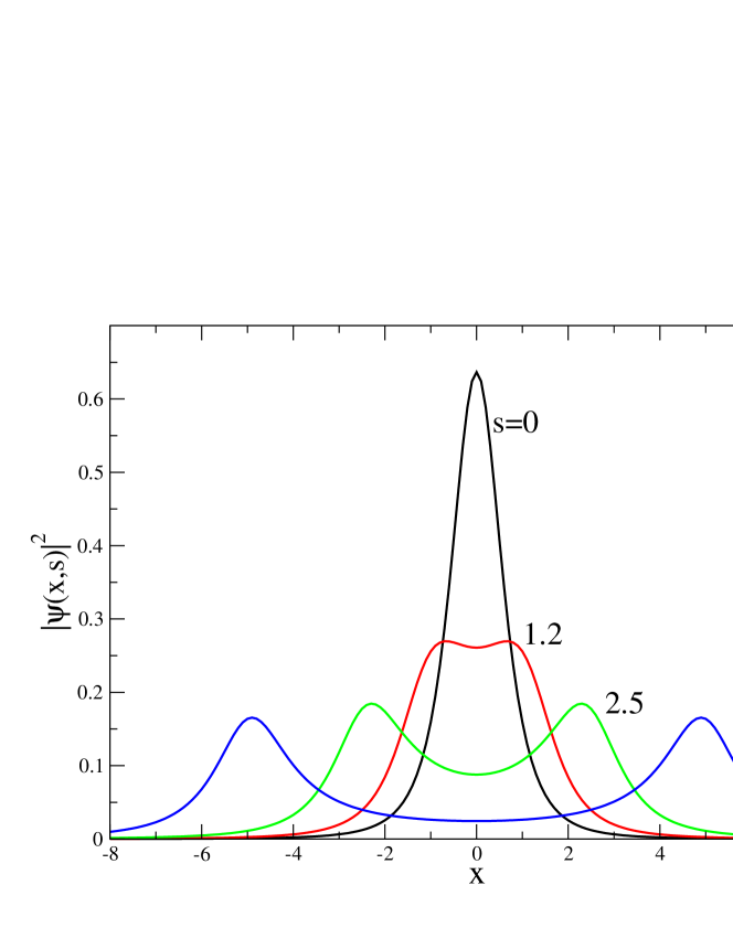
Figure 1: Time evolution of $\rho(x,t)=|\psi(x,t)|^{2}$, (95), for the Cauchy-Schrödinger dynamics (91) with the initial data (92). Figures near curves show time $t$ values.

By turning back to the semigroup transport formulas (34), (35) and 36) and directly executing the duality mapping $t\rightarrow it$ right there, we can easily discover an origin of the $\epsilon$-regularization, that is necessary if one attempts to deduce a consistent analytic expression for quasirelativistic and Cauchy quantum propagators. Let us focus on the Cauchy case again. The unitary dynamics of any $\psi(x,0)=f(x)$ is obtained as follows

$$\psi(x,t)=[\exp(-it|\nabla|)f](x)=(2\pi)^{-1/2}\int_{-\infty}^{+\infty}\exp(-it|k|+ikx)\,\tilde{f}(k)dk=(f*K_{t})(x)$$ (90)

where $(f*K_{t})(x):=\int K_{t}(x-z)f(z)dz$ and $K_{t}=(1/2\pi)\int\exp(-ikx-it|k|)\,dk$. As long as we do not insist on an explicit evaluation of the Fourier integral expression for $K_{t}(x)$, no regularization is necessary. The Fourier expression for $\psi(x,t)$ evidently does the job without any special precautions. On the other hand, would we have turned to $\psi(x,t)=(f*K_{t})(x):=\int K_{t}(x-z)f(z)dz$, it is only the regularized expression (85) that yields a time development of $\psi(x,t)$, in conformity with the Cauchy-Schrödinger equation, gar . The naive would-be propagator $K^{naive}_{t}(x)=it/\pi(x^{2}-t^{2})$, if taken literally, does not lead to a consistent evolution pattern, see below.

IV.5 Quantum wave packet dynamics in 1D

IV.5.1 Heavy-tailed initial data

With the propagator in hands, we can address the dynamical behavior of solutions of the free fractional (eventually Salpeter) Schrödinger-type equation. Lets us continue a discussion of the specific 1D Cauchy-Schrödinger case

$$i\partial_{t}\psi(x,t)=|\Delta|^{1/2}\psi(x,t)=|\nabla|\psi(x,t)$$ (91)

As an initial condition we take an ”almost Lorentz” (up to normalization) distribution, so that $|\psi|^{2}(x,0)$ actually is a normalized quadratic Cauchy pdf, gar2 :

$$\psi(x,0)=f(x)=\sqrt{\frac{2}{\pi}}\frac{1}{1+x^{2}}.$$ (92)

The integral kernel of $\exp(-i|\nabla|t)$ takes $\psi(x,0)$ into $\psi(x,t)$ through a convolution, c.f. Eq.  (36). For clarity of discussion we employ a regularized form $K_{t}^{\epsilon}(x)$ of the integral kernel, allowing to control its behavior in the vicinity of singularities, so arriving at

$$\psi(x,t)=f(x)*K^{\epsilon}_{t}(x)\equiv\int_{-\infty}^{\infty}f(x-z)K^{\epsilon}_{t}(z)dz=\frac{1}{2\pi}\sqrt{\frac{2}{\pi}}\int_{-\infty}^{\infty}\frac{dz}{1+(x-z)^{2}}\int_{-\infty}^{\infty}\ e^{-i(t-i\varepsilon)|u|}\cos uz\ du.\\$$

Consider $\quad I=\int_{-\infty}^{\infty}\frac{\cos uz\ dz}{1+(x-z)^{2}}=\pi e^{-|u|}\cos ux.\quad$ Thus, clearly

$$\psi(x,t)=\frac{1}{\sqrt{2\pi}}\int_{-\infty}^{\infty}e^{-|u|}\cos ux\ e^{-i(t-i\varepsilon)|u|}du\equiv\frac{1}{\sqrt{2\pi}}\int_{-\infty}^{\infty}e^{-|u|}e^{iux}e^{-i(t-i\varepsilon)|u|}du.$$ (93)

and an explicit evaluation of the integral, followed by $\varepsilon\to 0$, gives rise to

$$\psi(x,t)={\frac{1}{2}}[f(x+t)+f(x-t)]+{\frac{i}{2}}[(x-t)f(x-t)-(x+t)f(x+t)]=\sqrt{\frac{2}{\pi}}\frac{1+it}{(1+it)^{2}+x^{2}},$$ (94)

where $f(x)$ stands for the initial data (92) for the pertinent evolution. Taking the modulus of a complex function (94) we get interesting outcome, with an implicit redefinition $\rho^{1/2}_{0}(x)=f(x)$:

$$|\psi(x,t)|^{2}=(1+t^{2})\sqrt{\rho_{0}(x+s)\rho_{0}(x-s)}=\frac{2}{\pi}\frac{1+t^{2}}{\left[1+(x-t)^{2}\right]\left[1+(x+t)^{2}\right]},$$ (95)

which conveys a useful information about an enhanced spreading of the initial wave packet due to the dynamically generated bimodality of the square root expression. Compare e.g. horwitz ; gar ; cufaro ; remb . The pertinent time-evolution is visualized in Fig.1, compare e.g. also cufaro .

We would like to point out a definite advantage of the ($\epsilon$) regularized Fourier representation of the kernel which permits to incorporate naturally the delta-function terms and simplifies calculations. A complementary detailed derivation, explicitly accounting for delta-type contributions (85), can be found in Ref. gar .

IV.5.2 Link with a classical (d’Alembert) wave equation.

The solution (94) of Eq. (91) at the first glance seems to look like a general solution of the original equation of motion, represented as a superposition of special solutions (wave packets that are ”moving” right or left in the standard quantum lore), like e.g. $\Phi(x,t)=(1/\sqrt{2}[\phi(x-t)+\psi(x+t)]$, c.f. Eq. (3.37) in remb . This is merely an illusion and we must consider (94) as an indivisible whole, since no physical status can be assigned to separate right or left ”moving” components. This is a direct consequence of the manifest nonlocality of the motion generator $|\nabla|$.

Our standpoint is that there is no such entity as the right or left ”moving particle” in the present framework. That stays in plain opposition with a discussion of Sections 3 and 4 in Ref. remb . Even worse, the very ”particle” notion (concept) appears to be doubtful in this nonlocal dynamics setting, in view of the well known ”particle” (especially massless ”particle”) localization problems plaguing the relativistic quantum mechanics, c.f. for example Section V of Ref. gar and hawton ; ibb and references there-in.

Eqs (94) and (95) refer to a nonlocal complex-valued wave phenomenon, implying that the induced probability distribution bimodally expands and ultimately fades away (spreads). The underlying dynamical mechanism amounts to the propagation of local maxima, in the opposite directions, with the velocity of light (here $c=1$), (95). None of those maxima separately can be given a status of physical relevance, e.g. must not be interpreted as an identifier of a right or left ”moving particle” wave packet.

On the other hand the left- and right ”moving” components of (94) can be given a physical status within the higher level theory, i. e. the pure wave 1D d’Alembert equation $(-\Delta+{\frac{\partial^{2}}{\partial t^{2}}})u(x,t)=0$, where $c=1$. Both pertinent ”moving” components are solutions of this wave equation and likewise their superposition (94) is. The crux is that neither of component functions is by itself a solution of the Cauchy-Schrödinger equation. It is the ”indivisible whole”, i.e. their superposition $\psi(x,t)$ of Eq. (94), which for sure solves (91) and admits a standard quantum mechanical (Born’s) probabilistic interpretation.

It is worth pointing out that the Hilbertian domain of the operator $|\nabla|$ (containing all normalizable solutions of $\partial_{t}\psi=|\nabla|\psi$) can be consistently built by putting through a suitable sieve the set of all solutions of the 1D D’Alembert equation.  The pertinent domain is a fairly restrictively selected subset (closed linear space) of solutions of the d’Alemebert equation, such that the Cauchy-Schrödinger equation is solved by them as well (that we know not necessarily to be the case).

Remark: With Eq. (94) in hands we can be more explicit on the last sentence of the previous subsection. Namely, the Cauchy principal value of the (otherwise divergent) integral representing a ”naive” propagation $\psi(x,t)=(f*K^{naive}_{t})(x):=\int K^{naive}_{t}(x-z)f(z)dz$ of $\psi(x,0)=f(x)=\sqrt{2/\pi}/(1+x^{2})$ would result merely in the pure imaginary term $(i/2)[(x-t)f(x-t)-(x+t)f(x+t)]$ of the expression (94), which we know not to solve the Cauchy-Schrödinger equation as it stands, c.f. gar for more details.

IV.5.3 Dynamically generated bimodality

In view of Eqs. (94) and (95), a minor modification of the initial data (92) to $\psi(x.0)=\sqrt{\frac{2\gamma}{\pi}}\,[\gamma/{\gamma^{2}+x^{2}}]$, implies $\psi(x,t)=\sqrt{\frac{2\gamma}{\pi}}\left[(\gamma+it)/[(\gamma+it)^{2}+x^{2}]\right]$ and thence gives rise to the time-dependent pdf of the form

$$\rho(x,t)={\frac{2\gamma}{\pi}}{\frac{\gamma^{2}+t^{2}}{x^{4}+2x^{2}(\gamma^{2}-t^{2})+(\gamma^{2}+t^{2})^{2}}}\,.$$ (96)

We can quantify an emergence of bimodality by investigating an extremum of $\rho(x,t)$ with respect to $x$, i. e. solving an equation $\partial_{x}\rho=0$. This amounts to solving $x^{3}+x(\gamma^{2}-t^{2})=0$ with an obvious outcome: $x_{0}=0$, and two more real roots defined by $x_{\pm}=\pm\sqrt{t^{2}-\gamma^{2}}$ under the condition $t^{2}-\gamma^{2}>0$.

Accordingly, for times $t^{2}<\gamma^{2}$ the considered pdf is unimodal, while at time instants $t^{2}=\gamma^{2}=0$ the situation changes. The bimodal form od the pdf is born and persists for all $t^{2}>\gamma^{2}$. The pdf of the previous subsection is recovered by putting $\gamma=1$. We shall show subsequently that the reported behaviot of Cauhcy-Schrödinger pdfs is not due to a special choice of initial data. Additionally, we point out that the dynamical generation of bimodality is not special to the Cauchy-Schrödinger case and appears as well in the quasirelativistic (Salpeter) evolution.

Remark 1: There is no qualitative change in the behavior of solutions if we pass to the 1D quasirelativistic (Salpeter) equation $\partial_{t}\psi(x,t)=\sqrt{-\Delta+m^{2}}\psi(x,t)$. Initial data of the form

$$\psi(x,0)=\left[{\frac{m}{\pi K_{1}(2m\gamma)}}\right]^{1/2}{\frac{\gamma K_{1}(m\sqrt{x^{2}+\gamma^{2}})}{\sqrt{x^{2}+\gamma^{2}}}}$$ (97)

evolve in time according to a simple substitution rule $\gamma\rightarrow\gamma+it$. As well, one easily verifies that the $m\rightarrow 0$ limit reproduces the Cauchy-Schrödinger wave function, whose $|\psi|^{2}(x,t)$ is indeed the pdf $\rho(x,t)$ of Eq. (96), see e.g. usher ; remb ; cufaro . The denominator $\sqrt{x^{2}+(\gamma+it)^{2}}$ is a source of an emergent bimodality of this particular solution, as first noticed in Ref usher .

Remark 2: For both 1D Salpeter ($m>0$ and $m=0$) cases, a continuity equation $\partial_{t}\rho=-\nabla j$ has been verified to make sense and suitable probability currents are known in a closed analytic form, see e.g. remb .

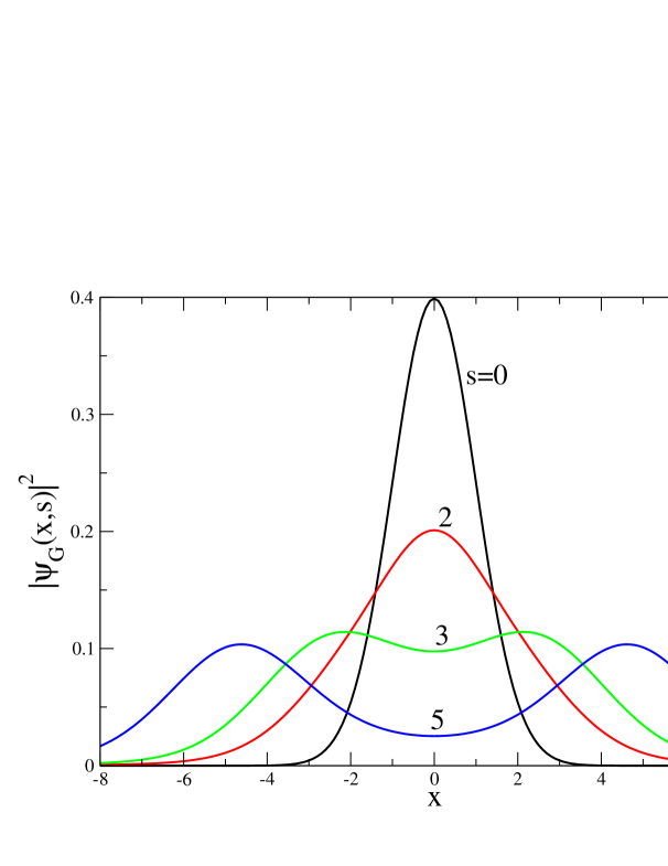
Figure 2: Time evolution of $\rho(x,t)=|\psi(x,t)|^{2}$ for the Cauchy-Schrödinger dynamics (100), with the initial data (98). Figures near curves show time $t$ values.

IV.5.4 Gaussian initial data

Now we consider the Cauchy-Schrödinger time evolution of the initial Gaussian wave packet, c.f. babusci for a complementary discussion of this issue,

$$\psi(x,0)=\frac{1}{\sqrt[4]{2\pi}}e^{-x^{2}/4}\,.$$ (98)

The dynamics is made explicit by employing the Fourier representation of $\psi(x,t)$. Namely, we have .

$$\psi(x,t)=\frac{1}{\sqrt{2\pi}}\int_{-\infty}^{\infty}\tilde{\psi}(u,t)e^{iux}du\equiv\frac{1}{\sqrt{2\pi}}\sqrt[4]{\frac{2}{\pi}}\int_{-\infty}^{\infty}e^{-u^{2}}\ e^{-it|u|}\ e^{\pm iux}du\equiv$$

$$=\left(\frac{2}{\pi}\right)^{3/4}\int_{0}^{\infty}\ e^{isz-z^{2}}\cos(zx)\ dz.$$ (99)

The integral can be evaluated exactly in terms of special functions to yield

$$\psi(x,t)=\sqrt[4]{\frac{2}{\pi}}\frac{e^{\frac{(x+t)^{2}}{4}}}{2\sqrt{2}}\left\{1+e^{tx}-i\left[e^{tx}{\rm erfi}\left(\frac{t-x}{2}\right)+{\rm erfi}\left(\frac{t+x}{2}\right)\right]\right\},$$ (100)

where ${\rm erfi}(x)=-i\ {\rm erf}(ix)$ is a real function.

We note in passing that following analytic methods of Ref. gar we would obtain another explicit form of the above $\psi(x,t)$:

$$\psi(x,t)=\frac{1}{2\sqrt[4]{2\pi}}\left\{\left[e^{-\frac{(x-t)^{2}}{4}}+e^{-\frac{(x+t)^{2}}{4}}\right]+\\ \frac{i}{2}P\left[\int_{-\infty}^{\infty}\frac{e^{-\frac{(x-y-t)^{2}}{4}}}{y}dy-\frac{e^{-\frac{(x-y+t)^{2}}{4}}}{y}dy\right]\right\}.$$ (101)

The squared modulus (e.g. a corresponding pdf) of the expression (100) (or (101)) is displayed in in Fig.2. A qualitative similarity between Gaussian and Cauchy (95) cases is transparent. Both functions exhibit a dynamically generated bimodality, see also cufaro . This behavior of $\psi(x,t)$ is definitely dictated by the propagator and appears not to depend on the initial data $\psi(x,0)$ choice.

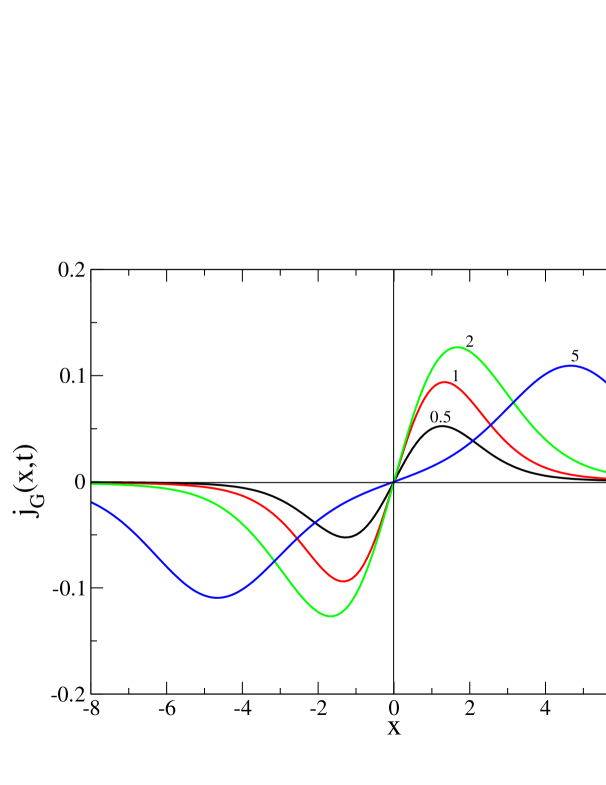
Figure 3: The probability current for an initially Gaussian distribution in the 1D Cauchy-Schrödinger dynamics. Figures near curves show the time $t$ values.

We finally note that there is no problem to deduce, with a numerical assistance if necessary, the detailed time evolution of any initial wave packet (Gaussian, Lorentzian etc) driven by a quasirelativistic kernel (e.g. proportional to the MacDonald function $K_{1}$).

Let us calculate the probability current for the present case (e.g. Gaussian initial data for the Cauchy-Schrödinger dynamics. To this end we shall employ the observations of remb . The Fourier transform of $\psi(x,0)=\frac{1}{\sqrt[4]{2\pi}}e^{-x^{2}/4}$ reads $\tilde{\psi}(p,0)=\sqrt[4]{\frac{2}{\pi}}e^{-p^{2}}$. The evolution can be encoded on the Fourier transform level as follows: $\tilde{\psi}(p,t)=\sqrt[4]{\frac{2}{\pi}}e^{-p^{2}-i|p|t}$. Next, we have to insert $\tilde{\psi}^{*}(p,t)$ and $\tilde{\psi}(k,t)$ to the defining identity (see e.g. subsection IV.E, here we scale away all dimensional constants and consider 1D instead of 3D):

$$j(x,t)={\frac{1}{2\pi}}\int_{-\infty}^{\infty}dp\int_{-\infty}^{\infty}dk\frac{p+k}{|p|+|k|}e^{ix(k-p)}\tilde{\psi}^{*}(p,t)\tilde{\psi}(k,t).$$ (102)

To facilitate the calculation of integral we pass to the polar coordinates $p=r\cos\varphi$, $k=r\sin\varphi$. Accordingly

$$j(x,t)=\frac{1}{\pi\sqrt{2\pi}}\int_{0}^{2\pi}\frac{\sin\varphi+\cos\varphi}{|\sin\varphi|+|\cos\varphi|}d\varphi\int_{0}^{\infty}re^{-r^{2}}e^{ixr(\sin\varphi-\cos\varphi)}e^{itr(|\cos\varphi|-|\sin\varphi|)}dr.$$ (103)

The integral in (103) can be evaluated analytically

$$J_{r}=\int_{0}^{\infty}re^{-r^{2}}e^{i\lambda r}dr=\frac{1}{2}\left\{1-\frac{\lambda\sqrt{\pi}}{2}e^{-\frac{\lambda^{2}}{4}}\left[-i+{\mathrm{erfi}}\left(\frac{\lambda}{2}\right)\right]\right\},\ \lambda(\varphi)=x(\sin\varphi-\cos\varphi)+t(|\cos\varphi|-|\sin\varphi|),$$ (104)

so that the final expression for the probability current assumes the form (cross-checked by means of Mathematica routines):

$$j(x,t)=\frac{1}{(2\pi)^{3/2}}\int_{0}^{2\pi}\frac{\sin\varphi+\cos\varphi}{|\sin\varphi|+|\cos\varphi|}\left\{1-\frac{\lambda(\varphi)\sqrt{\pi}}{2}e^{-\frac{\lambda(\varphi)^{2}}{4}}\left[-i+{\mathrm{erfi}}\left(\frac{\lambda(\varphi)}{2}\right)\right]\right\}d\varphi.$$ (105)

A numerical visualization of the time development of that current is reported in Fig. 3. It is seen that behavior of the current is qualitatively similar to that for the Cauchy initial packet, see e.g. Fig.2 in Ref. remb . Namely, at small times, there is practically no current at all (we begin from $j(x,t=0)=0$). The current is an odd function of $x$. As time passes, two positive and negative current peaks develop and move towards plus and minus infinities respectively, while falling down to zero.

IV.6 Quantum wave packet dynamics in 3D.

IV.6.1 Generic wave packet evolution pattern: radial expansion.

Peculiarities of the 3D dynamical behavior can be conspicuously seen in the Cauchy dynamics $i\partial_{t}\psi=|\nabla|\psi$, where due to the radial symmetry, the 1D bimodality is replaced by a ”spherical”-modality (and ”circular”-modality in 2D). The initial wave packet rapidly delocalizes by a dynamically developed expansion of a spherically-shaped probability concentration to the radial infinity, mimicking an expanding spherical wave with the source at the origin. Its radial peak is running away with the velocity $c$ (here interpreted as $c=1$): the pdf radial maximum resides on a surface of an expanding sphere (an expanding circle in 2D and an expanding interval in 1D).

This property can be directly deduced from the analytic formula ($r=\sqrt{x^{2}+y^{2}+z^{2}}$)

$$\psi(r,0)={\frac{(\sqrt{2\gamma})^{3}}{\pi}}{\frac{\gamma}{(r^{2}+\gamma^{2})^{2}}}\rightarrow\psi(r,t))={\frac{(\sqrt{2\gamma})^{3}}{\pi}}{\frac{\gamma+it}{[r^{2}+(\gamma+it)^{2}]^{2}}}$$ (106)

implying (set $\gamma=1$) the following functional form of the related pdf:

$$\rho(r,0)=|\psi(r,0)|^{2}={\frac{8}{\pi^{2}}}{\frac{1}{(1+r^{2})^{4}}}\longrightarrow\rho(r,t)=|\psi(r,t)|^{2}={\frac{8}{\pi^{2}}}{\frac{1+t^{2}}{[(r^{2}-t^{2}+1)^{2}+4t^{2}]^{2}}}$$ (107)

Its time evolution is depicted in Fig. 4. ($\gamma=1$, $r=\sqrt{x^{2}+y^{2}+z^{2}}$).

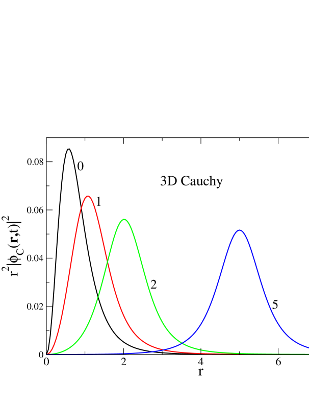
Figure 4: 3D Cauchy-Schrödinger evolution: spherical expansion, exemplified for the radial pdf $r^{2}\rho(r,t)$

We note that the normalization coefficient reflects the radial symmetry of the problem ($4\pi$ factor is the remnant of angular integrals), and Fig. 4 actually depicts the behavior of $r^{2}\rho(r,t)$, instead of the ”plain”$\rho(r,t)$. That should be compared with the time evolution pattern reported in Fig. 9 of remb .

The probability current for this case has received a closed analytic form in remb . Both the dynamical behavior and the rapid decay of $j(x,t)$ are depicted in Fig. 10 of remb .

Remark: Since a solution of the Cauchy-Schrödinger equation is also a solution of the D’Alembert equation (and not necessarily in reverse, c.f. subsection IV.E.2), it is worth pointing out that the pertinent wave equation is known to admit radially expanding (or contracting) spherical waves that originate from (or sink in) a point source (or sink). Superpositions of expanding and contracting waves are legitimate solutions as well.

IV.6.2 Propagators

In analogy to considerations of subsections III.C and IV.D, we may implement the quantum propagation $\psi(r,0)\rightarrow\psi(r,t)$ by means of the 3D propagator. To this end let us recall that the Cauchy kernel (transition probability density of the Cauchy jump-type process) stems form the general formula (41), specialized to $n=3$. Accordingly, while making explicit the $c$-dependence, we depart from

$$k_{0}({\bf x}-{\bf x^{\prime}},t-t^{\prime})={\frac{c(t-t^{\prime})}{\pi^{2}[({\bf x}-{\bf x^{\prime}})+c^{2}(t-t^{\prime})^{2}]^{2}}}={\frac{1}{(2\pi)^{3}}}\int d^{3}k\exp[-i{\bf k}({\bf x}-{\bf x^{\prime}})-|{\bf k}|c(t-t^{\prime})]$$ (108)

where $|{\bf k}|=\sqrt{k_{x}^{2}+k_{y}^{2}+k_{z}^{2}}$. For clarity of further discussion we shall keep in mind a space-time homogeneity of the corresponding random motion and retain ${\bf x}$ and $t$ labels, instead of ${\bf x}-{\bf x^{\prime}})$ and $t-t^{\prime}$ respectively.

The duality transformation $\exp(-c|\nabla|t)\rightarrow\exp(-ic|\nabla|t)$ can be accomplished on the level of integral kernels, provided we take care of potentially dangerous singularities (poles). Like before that can be secured by considering an $\epsilon$-regularized Cauchy-Schrödinger propagator in the form (compare e.g. also garcz ):

$$K^{\epsilon}_{t}({\bf x})={\frac{1}{(2\pi)^{3}}}\int d^{3}k\exp[-i{\bf k}{\bf x}-ic|{\bf k}|(t-i\epsilon)]\equiv{\frac{ict}{\pi^{2}[r^{2}-c^{2}(t-i\epsilon)]^{2}}}\,,$$ (109)

where $r=|{\bf x}|$. C. f. also our comment following Eq. (86) in regard to $\equiv$ versus $=$ in the above formula.

Perhaps it is instructive to mention (and make a direct comparison with Eq. (109) the so called complexified fundamental solution of the d’Alembert equation, ibb1 , which has the form (we set $\epsilon$ instead of the originally employed real constant $a$)

$$K_{\epsilon}({\bf x},t)={\frac{1}{c^{2}(t-i\epsilon)^{2}-r^{2}}}\,.$$ (110)

For $\epsilon\neq 0$ this function is analytic in the whole space-time. Would we proceed formally (it is not quite legal step in view of our discussion of the poles issue), and set $\epsilon=0$, one arrives at the Hadamard fundamental solution which is singular on the light cone.

Armed with the lesson of subsection III.D and the above (108) to (109) realization of the duality mapping, we know how to handle the arising singularity problems in the 3D ($m>0$) Salpeter case as well. Namely, the quasirelativistic jump-type process transition kernel (e.g. probability density, whose space-time homogeneity is implicit), in view of Eq. (40) reads

$$k_{m}({\bf x},t)={\frac{1}{(2\pi)^{3}}}\int d^{3}k\exp[-i{\bf k}{\bf x}-t(\sqrt{c^{2}{\bf k}^{2}+m^{2}c^{4}}-mc^{2})]=t\,{\frac{m^{2}c^{3}}{2\pi^{2}}}\exp(mc^{2}t)\,{\frac{K_{2}(mc\sqrt{r^{2}+c^{2}t})}{r^{2}+c^{2}t^{2}}}$$ (111)

where $K_{2}(z)\rightarrow 1/z^{2}$ for small values of $z$.

Accordingly, the $\epsilon$- regularized propagator of the 3D Salpeter equation $\partial_{t}\psi=(\sqrt{-c^{2}\Delta+mc^{2}}-mc^{2})\psi$ reads:

$$K^{\epsilon}_{m}({\bf x},t)\equiv it\,{\frac{m^{2}c^{3}}{2\pi^{2}}}\,\exp(mc^{2}it)\,{\frac{K_{2}(mc\sqrt{r^{2}-c^{2}(t-i\epsilon)})}{x^{2}-c^{2}(t-i\epsilon)^{2}}}$$ (112)

where $r=\sqrt{x^{2}+y^{2}+z^{2}}$ and $\hbar=1$ has been presumed. One may readily verify the validity of the $m\rightarrow 0$ limit, Eq,  (109).

IV.6.3 Probability currents in 3D

For the completeness of exposition we find instructive to present a detailed derivation of the probability current for the 3D Salpeter ($m\geq 0$) equation, whose main idea we borrow from Ref. remb . The transition to a simpler 1D case is obvious. We represent the Salpeter dynamics with an additive perturbation by an external potential

$$i\hbar\frac{\partial\psi}{\partial t}=\left[\sqrt{m^{2}c^{4}-\hbar^{2}c^{2}\Delta}+V({\bf x})\right]\psi$$ (113)

Accounting for

$$\psi^{*}\frac{\partial\psi}{\partial t}=-\frac{i}{\hbar}\left[\psi^{*}\sqrt{m^{2}c^{4}-\hbar^{2}c^{2}\Delta}\ \psi+V({\bf x})\psi^{*}\psi\right].$$ (114)

and its complex conjugate we can evaluate the time derivative of the probability density $\rho=|\psi|^{2}$ according to $\frac{\partial(\phi^{*}\psi)}{\partial t}=\psi\frac{\partial\psi^{*}}{\partial t}+\psi^{*}\frac{\partial\psi}{\partial t}$ so that

$$-\frac{\partial|\psi|^{2}}{\partial t}=\frac{i}{\hbar}\left[\psi^{*}\sqrt{m^{2}c^{4}-\hbar^{2}c^{2}\Delta}\,\psi-\psi\sqrt{m^{2}c^{4}-\hbar^{2}c^{2}\Delta}\,\psi^{*}\right].$$ (115)

Our aim is to transform (115) into a regular 3D continuity equation $-\frac{\partial\rho}{\partial t}$$=\nabla{\bf j}$, $\rho=|\psi|^{2}$. Taking the Fourier transforms of each $\psi$- entry in the right-hand-side of (115) separately, and presuming that the r-h-s actually stands for $\nabla{\bf j}$, we get

$$\nabla{\bf j}={\frac{ic}{(2\pi)^{3}\hbar^{7}}}\int d^{3}p\,\,d^{3}k\,[\phi^{*}_{p}\sqrt{m^{2}c^{2}+k^{2}}\,\phi_{k}-\phi_{k}\sqrt{m^{2}c^{2}+p^{2}}\,\phi_{p}^{*}]\,e^{i{\frac{{\bf x}}{\hbar}({\bf k}-{\bf p}}})=$$ (116)

$${\frac{ic}{(2\pi)^{3}\hbar^{7}}}\int d^{3}p\,\,d^{3}k\,\phi^{*}_{p}\phi_{k}\left[{\frac{k^{2}-p^{2}}{\sqrt{m^{2}c^{2}+k^{2}}+\sqrt{m^{2}c^{2}+p^{2}}}}\right]e^{i{\frac{{\bf x}}{\hbar}({\bf k}-{\bf p}}})\,.$$ (117)

In view of $({\bf k}+{\bf p})({\bf k}-{\bf p})=k^{2}-p^{2}$, we readily retrieve the functional (spectral) expression for $\bf j$ that obeys the continuity equation:

$${\bf j}=\frac{c}{(2\pi)^{3}\hbar^{6}}\int d^{3}p\ d^{3}k\frac{{\bf k}+{\bf p}}{\sqrt{m^{2}c^{2}+k^{2}}+\sqrt{m^{2}c^{2}+p^{2}}}\phi^{*}_{p}\phi_{k}e^{i\frac{{\bf x}}{\hbar}({\bf k}-{\bf p})}$$ (118)

The massless case arises if we set $m=0$ in (118). The probability current for the massless case reads

$${\bf j}=\frac{c}{(2\pi)^{3}\hbar^{6}}\int d^{3}p\ d^{3}k\frac{{\bf k}+{\bf p}}{|{\bf k}|+|{\bf p}|}\phi^{*}_{p}\phi_{k}e^{i\frac{{\bf x}}{\hbar}({\bf k}-{\bf p})}.$$ (119)

To have a direct comparison with some of our previous discussions, one should set $\hbar=1=c$ whenever necessary.

Remark: In the present subsection we have discussed the quasirelativistic generator that is additively perturbed by a function (like e.g. a Newtonian potential) that secures a bounded-ness of the Hamiltonian in (113) from below and (via an additive renormalization) moves its spectrum to $R_{+}$, with $0$ as its lowest eigenvalue. A number of typical (e.g. simplest) spectral problems have been addressed in the past both for the 3D and 1D quasirelativistic cases, remb1 ; lucha ; lucha1 ; lucha2 ; kaleta and references there-in. Some special spectral problems (harmonic potential and the infinite well case) for the $m=0$, were considered e.g. in laskin ; laskin1 ; remb1 ; gar1 ; gar2 ; malecki and jeng ; baym ; hawkins . There are open problems even in those simple cases; controversies concerning an analytic form of eigenfunctions and the ground state function in particular have not been resolved for a ”particle in a box”, laskin ; baym ; hawkins . Mathematical arguments kwasnicki , indicate that none of proposed so far solutions is correct, as confirmed in the very recent Ref. luchko .

IV.6.4 Non-existence of the continuity equation for the fractional quantum dynamics.

In the standard quantum mechanics, where the minus Laplacian is recognized to serve also as the Wiener noise generator, the time derivative of $\rho$ is routinely represented in terms of the continuity equation. The argument goes as follows: consider a normalized solution of the Schrödinger equation (we set here-by $\hbar/2m=1$), then $\partial_{t}|\psi|^{2}=i[\psi^{*}(\nabla^{2})\psi-\psi\nabla^{2}\psi^{*}]=i\nabla(\psi^{*}\nabla\psi-\psi\nabla\psi^{*})=-\nabla j$.

If we consider the $\mu$-stable generator instead of the minus Laplacian, a consequence of the Lévy-Schrödinger equation is: $\partial_{t}|\psi|^{2}=-i(\psi^{*}|\Delta|^{\mu/2}\psi-\psi|\Delta|^{\mu/2}\psi^{*})$. This equation readily applies to the $|\nabla|=|\Delta|^{1/2}$ and extends to the Salpeter generator $\sqrt{-\Delta+m^{2}}$, whose mass $m=0$ version the Cauchy generator actually is. The just derived 3D version of the probability current can be associated with those two special cases.

The situation appears more troublesome when general Lévy-stable generators $|\Delta|^{\mu/2}$ are involved. We note that in this case there holds (we refer to 3D, dimensional constants are scaled away)

$$-\frac{\partial|\psi|^{2}}{\partial t}=\frac{i}{\hbar}\left[\psi^{*}|\Delta|^{\mu/2}\,\psi-\psi|\Delta|^{\mu/2}\,\psi^{*}\right]={\frac{i}{(2\pi)^{3}}}\int d^{3}p\,\,d^{3}k\,{\frac{|k|^{2\mu}-|p|^{2\mu}}{|k|^{\mu}+|p|^{\mu}}}\,\phi^{*}_{p}\,\phi_{k}e^{i{\frac{{\bf x}}{\hbar}({\bf k}-{\bf p}}}).$$ (120)

and there is no way to extract the crucial factor ${\bf k}-{\bf p}$, needed to identify (120) as a legitimate (spectral) expression for $\nabla{\bf j}$ , with a notable exception of $\mu=1$.

A candidate expression for the probability current, albeit restricted to the stability parameter range $\mu\in(1,2)$, has been produced in Ref. (laskin ; laskin1 , see also an explicitly uncompleted passage from (38) to (39) in dong . While setting $\hbar\equiv 1$ and disregarding the noise intensity parameter $D_{\mu}$, ${\bf j}$ has been presented in the form:

$${\bf j}=-i\psi^{*}|\Delta|^{\mu/2-1}\nabla\psi-\psi|\Delta|^{\mu/2-1}\nabla\psi^{*}$$ (121)

The problem is that the identity $\partial_{t}\rho=-\nabla{\bf j}$ is invalid as it stands, in its differential form, e.g. there is no $-div{\bf j}$ local representation of $\partial_{t}\rho$. This can be demonstrated by inspection after passing to the spectral representation.

Our negative argument goes as follows, zaba . First we observe that by taking the divergence of ${\bf j}$, (121), we get

$$\nabla{\bf j}=-i\left[(\nabla\psi^{*})\,|\Delta|^{\mu/2-1}\nabla\psi-(\nabla\psi)\,|\Delta|^{\mu/2-1}\nabla\psi^{*}\right]-i\left[\psi^{*}\,\nabla|\Delta|^{\mu/2-1}\nabla\psi-\psi\,\nabla|\Delta|^{\mu/2-1}\nabla\psi^{*}\right]$$ (122)

Now, we shall consider the second square-bracketed term in the above. To this end let us explicitly evaluate the action of involved operators, while passing to the spectral (Fourier) representation of the relevant entry. We have e.g.

$$\psi^{*}\,\nabla|\Delta|^{\mu/2-1}\nabla\psi=-\psi^{*}({\bf x}){\frac{1}{(2\pi)^{3/2}}}\int d^{3}p\,|p|^{\mu}e^{i{\bf px}}\,\tilde{\psi}({\bf p})=-\psi^{*}|\Delta|^{\mu/2}\psi$$ (123)

and taking into account a complex conjugate of (123), we recover the right-hand-side of the transport equation (120), (up to $\hbar\equiv 1$ and an obvious sign inversion). For ${\bf j}$ of Eq. (121) to be a legitimate probability current we must guarantee that the first square bracketed term of Eq. (122) identically vanishes. This is not the case for complex functions $\psi$.

Remark: It has been demonstrated in gar , c.f. also angelis , that the transport equation $\partial_{t}|\psi|^{2}=-\frac{i}{\hbar}\left[\psi^{*}|\Delta|^{\mu/2}\,\psi-\psi|\Delta|^{\mu/2}\,\psi^{*}\right]$ can be literally represented as a master-type equation for the jump-type process with a corresponding jumping rate $q({\bf x},t,A)$ where $A$ is a Borel set in $R^{3}$. The pertinent master-type equation has the form $\partial_{t}\rho(A,t)=\int q({\bf y},t,A)\,\rho({\bf y},t)\,d^{3}y$ and $q({\bf x},t,A)$ critically depends on the involved Lévy measure. If $\rho({\bf x},t)$ is a probability density of a certain stochastic process, then $\int_{A}\rho(x,t)d^{3}x=\rho(A,t)$ tells us what is the probability for a jump to have its spatial direction and size matching ${\bf x}\in A$. However, one should not be inclined to think that a concrete jump refers to a ”physical particle” that jumps in space. We shall leave this debatable point open for further discussion. To the contrary, in a conventional Laplacian-based quantum mechanics, a standard interpretation of $\rho({\bf x},t)(\Delta x)^{3}$ as a probability to locate a ”physical particle” in a cube of volume $(\Delta x)^{3}$ seems to be consistent.

V Domains for nonlocal operators, state vectors and uncertainty relations

V.1 Mathematical prerequisites

Hamiltonian operators discussed in this paper are unbounded. When defining an unbounded operator, it always is necessary to specify its domain of definition. We proceed in he following general manner. If $A$ is an operator in the Hilbert space ${\cal{H}}$, we write $D(A)\subset{\cal{H}}$ for the domain of $A$.

Let us consider a densely defined self-adjoint operator $A$. For any $g\in D(A)$, we set

$$||g||_{A}=[(Ag,Ag)+(g,g)]^{1/2}\,.$$ (124)

Then $||\cdot||_{A}$ is a norm in $D(A)$. As well, we consider $(f,g)_{A}=(Af,Ag)+(f,g)$ to be a scalar product specific to $D(A)$.

If $f_{n}\in D(A)$ is a Cauchy sequence in $||\cdot||_{A}$, that is, $\lim_{n,m\rightarrow\infty}||f_{m}-f_{n}||_{A}=0$, then $f_{n}$ also is a Cauchy sequence in the Hilbert space ${\cal{H}}$ norm $||f||=[(f,f)]^{1/2}$. By the completeness of ${\cal{H}}$ there is $f\in{\cal{H}}$ such that $\lim_{n\rightarrow\infty}||f-f_{n}||=0$. It follows that $f$ necessarily belongs to $D(A)$ (that is, $D(A)$ is complete in the $||\cdot||_{A}$ norm). Then $A=A^{*}$ is closed and denoted $A=\overline{A}$. (The closedness is a consequence of $D(A)=D(A^{*})$ and an assumption that D(A) is dense in ${\cal{H}}$, karw1 .)

In our text, we have introduced Hamiltonian-type operators $\hat{H}=\hat{H}_{0}+V$, where $\hat{H}_{0}$ is a nonlocal generator of Lévy noise, via a canonical quantization of the Lévy-Khintchine formula. Consequently, we encounter standard quantum mechanical domain problems for unbounded operators. This refers as well to $\hat{H}$ and position-momentum (fairly standard !) operators $\hat{x},\hat{p}=-i\nabla$ which form a canonical pair $[\hat{x},\hat{p}]\subset iI$, up the presence of $\hbar$ which in various parts of the paper has been identified with unity..

Let us take Hilbert space vectors $f,g\in L^{2}$ and let $(f,g)\in C$ represent a standard scalar product in the complex functions space. We need

$$(f,\hat{H}g)=(f,\hat{H}_{0}g)+(f,Vg)$$ (125)

to have granted the existence status (e. g. the convergence of involved integrals). In particular, if $f$ is a normalized function, we may expect the mean energy value $(f,\hat{H}f)=\langle H_{0}\rangle+\langle V\rangle$ here-by defined up to dimensional constants, to exist. Since our main objective are domain issues for $\hat{H}_{0}$, let us set $V=0$ and pay attention to $(f,\hat{H}_{0}g)$ exclusively.

In passing we note that in reference to the semigroup dynamics and the associated jump-type processes, a well developed mathematical formalism of Dirichlet forms associated with noise generators $-\hat{H}_{0}$ is available, lorinczi ; liming ; chen . The pertinent quadratic forms ”live” in a Hilbert space of real-valued functions. This subject matter has been also addressed in the physics-oriented literature but exclusively in relation to $-\Delta$, i. e. in the context of the Wiener noise and the emergent semigroup description of the Brownian motion, albeverio .

We are somewhat guided by basic tenets of that theory, but our considerations will refer directly to the unitary (quantum) dynamics and therefore our Hilbert space contains complex valued $L^{2}$ functions, the real ones forming merely a subset in $L^{2}$ and not a linear subspace, karw .

All symmetric Lévy noise generators are Hermitian (actually self-adjoint, applebaum ), $(f,\hat{H}_{0}g)=(\hat{H}_{0}f,g)$, on their domains od definition. They are also non-negative. Therefore their operator square roots are always well defined as self-adjoint operators.

Accordingly, we can pose an auxiliary domain problem for $H_{0}^{1/2}$, by considering

$$(f,\hat{H}_{0}g)=(\hat{H}_{0}^{1/2}f,\hat{H}_{0}^{1/2}g)$$ (126)

as a relevant (e.g. non-trivial) part of the induced scalar product $(f,g)_{H_{0}^{1/2}}$ in $D(H_{0}^{1/2})\subset L^{2}$, c.f. Eq. (124).

The operator domain of interest would consist of all $f$ and $g$ in $L^{2}$, such that the completion of a corresponding linear space in the $\|.\|_{\hat{H}^{1/2}_{0}}$ norm would identify a closed dense subspace of $L^{2}$. We shall not be more elaborate on purely mathematical issues and assume such domain existence for granted, for each self-adjoint $\hat{H}_{0}$ of Section III separately.

V.2 Test model: Quasirelativistic Hamiltonian.

As a test model let us consider the quasirelativistic Hamiltonian $H_{m}=\sqrt{m^{2}-\Delta}-m$, ($\hbar=c=1$). We know that solutions of the Salpeter equation

$$i\hbar\frac{\partial\psi(\mathbf{x},t)}{\partial t}=[\sqrt{m^{2}-\Delta}-m]\ \psi(\mathbf{x},t)$$ (127)

have the form $\psi(\mathbf{x},t)=\exp(imt)\,\phi(\mathbf{x},t)$. Therefore, instead of introducing the domain for $H_{m}$ proper, which is a nonnegative operator (with $0$ as the bottom generalized eigenvalue), we may pass to an equivalent domain analysis, carried out for the strictly positive operator $H_{m}+m=\sqrt{m^{2}-\Delta}$, see e.g. our discussion of Section IV.B.2.

This step is advantageous, since if $\psi(\mathbf{x},t)$ is a solution of the pseudodifferential–Schrödinger equation $i\partial_{t}\psi=[\sqrt{-\Delta+m^{2}}-m]\psi$, then $\phi(\mathbf{x},t)=\psi(\mathbf{x},t)\exp(-imt)$ necessarily is a positive energy solution of the free Klein-Gordon equation $(\Box+m^{2})\phi(\mathbf{x},t)=0$, with $\Box=-\Delta+\partial^{2}/\partial t^{2}$.

Each scalar positive energy solution $\phi(\mathbf{x},t)$ of the free Klein-Gordon equation can be represented in the manifestly Lorentz covariant form:

$${\phi(\mathbf{x},t)={1\over{(2\pi)^{3/2}}}\int d^{4}k\,e^{(-ik_{\mu}x^{\mu})}\,\delta(k_{\mu}k^{\mu}-m^{2})\Theta(k_{0})\,\Phi(k_{0},\mathbf{k})}={\frac{1}{(2\pi)^{3}}}\int{\frac{d^{3}k}{k_{0}}}\Phi(k_{0},\mathbf{k})e^{(-itk_{0}+i\mathbf{k}\mathbf{x})}$$ (128)

where $k:=(k_{0},\mathbf{k})$, $k_{\mu}k^{\mu}:=k_{0}^{2}-\mathbf{k}^{2}$, $\Phi(k)$ is a scalar and $\Theta(k_{0})$ is the Heaviside function equal to $1$ if $k_{0}>0$ and to $0$ otherwise. Ultimately we are left with $k_{0}=\sqrt{\mathbf{k}^{2}+m^{2}}$.

This representation extends to all solutions of $i\partial_{t}\phi=\sqrt{-\Delta+m^{2}}\phi$, and upon changing $k_{0}\to-k_{0}$ in $\Theta(k_{0})$ followed by a complex conjugation, to solutions of the time adjoint equation as well. (Side comment: general solutions of those pseudodifferential–Schrödinger equations form Lorentz invariant subspaces in the linear space of all solutions to the free Klein-Gordon equation.)

Let us tentatively adopt the following definition of the Klein-Gordon scalar product, barut , (being independent of the specific space-like surface of integration):

$${(\phi_{1},\phi_{2})_{KG}:={\frac{i}{2}}\int_{R^{3}}d^{3}x\,[\overline{\phi_{1}}\partial_{t}\phi_{2}\,-\partial_{t}\overline{\phi_{1}})\phi_{2}]}.$$ (129)

Given positive energy solutions of the free Klein-Gordon equation $\phi_{i}(x),i=1.2$, which we know to solve the quasirelativistics equation as well, we realize that ($\tilde{\phi}_{i}$ is a Fourier transform of $\phi_{i}$)

$$(\phi_{1},\phi_{2})_{KG}=\int{\frac{d^{3}k}{k_{0}}}\tilde{\phi_{1}}^{*}\tilde{\phi}_{2}=(\phi_{1},\sqrt{-\triangle+m^{2}}\phi_{2})=((-\triangle+m^{2})^{1/4}\phi_{1},(-\triangle+m^{2})^{1/4}\phi_{2})$$ (130)

We recall that $\sqrt{-\triangle+m^{2}}$ is a Hermitian operator in the Hilbert space $L^{2}$, equipped with a scalar product $(\phi_{1},\phi_{2})=\int d^{3}x\overline{\phi}_{1}(\vec{x},t)\phi_{2}(\vec{x},t)$.

We can now introduce a new positive energy solution for both Klein-Gordon and quasirelativistic Schrödinger equations as follows

$$\phi(x)\to[(-\Delta+m^{2})^{1/4}\phi](x).$$ (131)

At this point we consider $\phi$ as the $L^{2}$-normalized function in the domain of $(m^{2}-\Delta)^{1/4}$, so arriving at the mean energy of the quantum system in the state $\phi$ (to be compared with Eq. (126)):

$$((m^{2}-\Delta)^{1/4}\phi,(m^{2}-\Delta)^{1/4}\phi)=(\phi,(m^{2}-\Delta)^{1/2}\phi)=E_{\phi}>0.$$ (132)

Accordingly,

$$\Phi=(1/\sqrt{E_{\phi}})(m^{2}-\Delta)^{1/4}\phi$$ (133)

is $L^{2}$ normalized, $(\Phi,\Phi)=1$. (We remember that $(\phi,\phi)=1\rightarrow(\phi,\phi)_{KG}=E_{\phi}$).

The $L^{2}$ normalized function $\Phi$ may serve as a reference state that gives account of the energy spatial distribution, c.f. barut ; ibb ; ibb1 . The reverse operation obviously reads $\phi=\sqrt{E_{\phi}}(m^{2}-\Delta)^{-1/4}\Phi$.

Introducing the pdf $\rho({\bf x},t)=|\Phi|^{2}({\bf x},t)$ we have in hands a probability measure. Let $\Omega$ be a volume in $R^{3}$. Then, we interpret $p_{E}(\Omega)=\int_{\Omega}d^{3}x\,|\Phi|^{2}$ as a fraction of the total mean energy $E_{\phi}$ that is confined in the volume $\Omega$. Compare e.g. analogous considerations in the context of the photon wave mechanics in ibb ; ibb1 .

We note in passing that the way we have introduced $\Phi$ stays in an intimate relationship with the (induced) notion of the Newton-Wigner position operator, barut ; jordan although this notion appears to be irrelevant for our discussion, compare also gar .

In particular, we emphasize that the canonical quantization method adopted by us relies on the standard position-momentum pair $[x_{j},p_{k}]\subset\delta_{ij}I$, with $\vec{p}=-i\vec{\nabla}$. Accordingly, most familiar uncertainty relations hold true $\Delta x\Delta p\geq 1/2$. One may merely enter a dispute of what are the states that may sharpen the Heisenberg bound. No new position operator notions are here necessary (c.f. past discussions of the covariant position operator notion and the causality issue in relativistic quantum theory).

Our test model discussion allows us to come to a general conclusion. Let us disregard introductory KG equation hints (126)-(130). Then, the mean energy-based probability measure definitions (131), (132) can be readily extended (up to dimensional coefficients) to any Lévy stable case. To this end one needs to begin with the mean energy definition in a given state and replace the quasirelativistic operator $\sqrt{m^{2}-\Delta}$ in defining formulas (131) and (132) by a fractional operator $|\Delta|^{\mu/2}$ with $\mu\in(0,2)$.

Clearly, any connection with standard (relativistic) wave equations is lost, with a notable exception of the Cauchy case $\mu=1$, where the D’Alembert link persists. In the latter context, let us assume that the function $\Phi(k_{0},{\bf k}$ in Eq. (128) is selected so that under the $m\downarrow 0$ limit, $(1/|\mathbf{k}|)\Phi(|\mathbf{k}|,\mathbf{k})$ has the property to vanish if we let $|\mathbf{k}|$ go down to $0$. Then, all arguments following Eq. (128) retain their validity, if we replace $(-\Delta+m^{2})^{1/n}$ by $|\Delta|^{1/2n}$ everywhere, for $n=1,2$.

V.3 Foldy’s synthesis for $m>0$ and its $m=0$ extension to photon wave mechanics.

Let us come back to the Salpeter equation in its $m\geq 0$ versions. The link of the $m>0$ equation with various relatvistic equations has been established long time ago under the name of Foldy’s ”synthesis of covariant particle equations”, foldy , see also simulik . It has been shown that Dirac, Klein-Gordon and Proca equations can be reduced to a canonical form

$$i\partial_{t}\chi=\sqrt{-\Delta+m^{2}}\,\beta\,\chi$$ (134)

where $\beta$ is a diagonal hermitian matrix. In particular, solutions $\phi$ of the Klein-Gordon equation $(\Box+m^{2})\phi(\vec{x},t)=0$ yield a two-component wave function $\chi$ with components $\chi_{\pm}=(1/\sqrt{2})[(-\Delta+m^{2})^{-1/4}\partial_{t}\phi\mp i(-\Delta+m^{2})^{1/4}\phi]$. The matrix $\beta$ is identical with the Pauli matrix $\sigma_{3}$, comprising $1$ and $-1$ on the diagonal.

The reduction of the Dirac equation to the canonical form is accomplished by the Foldy-Wouthuysen (FW) transformation. Let $\psi$ be a solution of

$$i\partial_{t}\psi=(\beta m-i\vec{\alpha}\cdot\vec{\nabla})\,\psi\,.$$ (135)

The canonical form (134) is obeyed by the four-component $\chi=U\psi$ where $U$ stands for the F-W transformation, while $\beta$ comes from the Dirac equation in its traditional block-diagonal form, comprising the $2\times 2$ identity matrix $I$ and its negative $-I$.

The Proca equation adopted in foldy leads to a canonical form with a $6$-component $\chi$ and $\beta$ being being block-diagonal with $3\times 3$ blocks $I$ and $-I$.

The case of mass $m=0$ has been properly addressed quite recently, being associated with attempts to give meaning to the (single) photon wave mechanics, ibb ; ibb1 ; ibb2 , see also garcz . The key element there was a reformulation of Maxwell equations in terms of the Riemann-Silberstein vector function ${\bf F}({\bf x},t)$, actually interpreted as the R-S wave function, e.g. a solution of the Schrödinger-type equation with a divergence constraint

$$i\partial_{t}{\bf F}=c\nabla\times{\bf F}$$ (136)

$$\nabla\cdot{\bf F}=0\,.$$ (137)

The above dynamical equation can be given more explicit Schrödinger form by invoking spin $1$ ($3\times 3$, no $\hbar$ involved) matrices $[S_{j},S_{k}]=i\epsilon_{jkl}S_{l}$, so that c.f. ibb

$$i\partial_{t}{\bf F}={\frac{c}{i}}({\bf S}\cdot\nabla){\bf F}$$ (138)

We note that the divergence condition excludes the potentially troublesome $\vec{k}=\vec{0}$ mode. Therefore we can safely introduce the inverse of the Cauchy operator $|\Delta|^{1/2}$, while acting upon $\bf F$ such that $\nabla\cdot{\bf F}=0$.

By introducing the helicity operator $\hat{\Lambda}$ for photons (loosely speaking, a projection of spin on momentum) which is a manifestly nonlocal operator, we can rewrite the photon Hamiltonian $\hat{H}=\hat{\bf p}\cdot\hat{\bf S}$ as follows

$$\hat{H}=c|\hat{\bf p}|\,\hat{\Lambda}$$ (139)

$$\hat{\Lambda}={\frac{1}{|\nabla|}}(\hat{\bf p}\cdot\hat{\bf S})$$ (140)

where $\hat{\bf p}=-i\nabla$ and we interpret $|\hat{\bf p}|$ as $|\nabla|=|\pm\Delta|^{1/2}$. We can pass to the helicity basis (with the corresponding eigenvalues $\pm 1$), ending with positive energy solutions of the $m=0$ variant of the Salpeter equation, in the canonical form

$$i\partial\chi=c|\Delta|^{1/2}\beta\chi$$ (141)

where $\beta$ is the $6\times 6$ diagonal matrix, encountered before in connection with the Proca equation. Here, $\chi$ is a $6$-component vector composed of positive frequency pieces taken form the original R-S vector and its complex adjoint, i. e. ${\bf F}^{(+)}$ and ${\bf F}^{(-)*}$ respectively. Compare a discussion of the helicity /spin spectral issues in Section 2.1 of ibb , see also garcz .

In the helicity basis, the photon wave function dynamics is nonlocal and shows all intriguing features (radial expansion) discussed before in subsection III.F.1. We note that the expanding/contracting behavior has been previously associated with the photon energy density ${\bf F}\cdot{\bf F}^{*}$, see e.g. Fig. 3 in ibb1 . A discussion of involved uncertainty relations, from varied perspectives, including the mean energy normalization of the wave function, can be found in ibb ; ibb1 ; ibb2 , see specifically Eqs. (5.28)-(5.31) of Ref. ibb ). Their obvious validity is not that illuminating as a useful indicator delocalization in view of rather rapid radial expansion of wave packets.

By invoking the scalar product considerations of Section 5.1 in ibb we readily arrive at the $m=0$ version of the interplay between solutions of the second order wave equations (here, d’Alembert) and those inferred from the Schrödinger type equation. Namely, the inversion relation $\phi=\sqrt{E_{\phi}}(m^{2}-\Delta)^{-1/4}\Phi$ of subsection IV.B has a counterpart in the photon wave mechanics. Up to the mean energy normalization, the Landau-Peierls wave function $\phi=|-\Delta|^{-1/4}\Phi$ (c.f. section 5.3 in ibb ) is precisely the outcome of a mapping of solutions of the d’Alembert equation, $({\frac{1}{c^{2}}}{\frac{\partial^{2}}{\partial t^{2}}}-\Delta){\bf F}_{\pm}=0$, (128) (set m=0 therein), to $L^{2}$ normalized solutions of Eqs. (138) and /or (141).

To be more explicit, we note that all previous steps (129) through (130) can be safely repeated if: (i) in view of $m=0$, we replace $(-\triangle+m^{2})^{1/2n}$ by $|\triangle|^{1/2n}$, with $n=1,2$, (ii) next extend the interpretation of integration to encompass summmation over helicity indices $\lambda=1,-1$, and (iii) insert $\Phi_{\lambda}(k_{0},\vec{k})$ instead of the previous $\Phi(k_{0},\vec{k})$.

Then the ($m\downarrow 0$) KG scalar product (129) assumes the d”Alembertian form and refers to two-component positive energy solutons of both d’Alembert and the Cauchy-Schrödinger equation (here we consider the squared norm of $\phi$ ):

$$(\phi,\phi)_{d^{\prime}A}=\sum_{\lambda}\int{\frac{d^{3}k}{k_{0}}}\tilde{\phi_{\lambda}}^{*}\tilde{\phi}_{\lambda}=(\phi,|\triangle|^{1/2}\phi)=(|\triangle|^{1/4}\phi,|\triangle|^{1/4}\phi)=E_{\phi}$$ (142)

and the $L^{2}$ normalization of a positive energy solution $(\phi,\phi)=1$ clearly implies $(\phi,\phi)_{d^{\prime}A}=E_{\phi}$ and the $L^{2}$ normalization $({\bf\Phi},{\bf\Phi})=1$ of

$${\bf\Phi}=(1/\sqrt{E_{\phi}})|\Delta|^{1/4}\phi\,.$$ (143)

Now we are exactly at the point where the Landau-Peierls (LP) wave function happens to be introduced. This issue was a subject of disagreements in the literature, that ranged form accepting to discard th L-P functions as an object of a physical relevance, good ; ibb . On the basis of (142), (143), we know that both ${\bf\Phi}$ and $\phi$ are fairly legitimate objects.

However if ${\bf\Phi}$ is what we interpret to provide a consistent probabilistic interpretation of a single photon quantum state (see e.g. also sections 5 and 5 of ibb and good ), then we may always reproduce $\phi$ with the squared norm $(\phi,\phi)_{d^{\prime}A}=\sum_{\lambda}\int{\frac{d^{3}k}{k_{0}}}\tilde{\phi_{\lambda}}^{*}\tilde{\phi}_{\lambda}$ according to $\phi=\sqrt{E_{\phi}}|\Delta|^{-1/4}\Phi$. We recall that $(\phi,\phi)=1\rightarrow(\phi,\phi)_{d^{\prime}A}=E_{\phi}$. Hence $\phi/\sqrt{E_{\phi}}$ is d’Alembert-normalized. That can also be accomplished by writing

$${\frac{1}{E_{\phi}}}(\phi,\phi)_{d^{\prime}A}=(|\Delta|^{-1/4}\phi,|\Delta|^{-1/4}\phi)_{d^{\prime}A}=1\,.$$ (144)

We note that often expressed in the literature past prejudices, concerning the LP wave function nonlocality (reaching back to W. Pauli, (1933), ibb ), in the light of our discussion must be taken under scrutiny as invalid objections. All ingredients of our theory of quantum motion are spatially nonlocal. That is possibly somewhat blurred on the Fourier level of description, but fairly obvious while invoking the primary level of of the theory, based on the exploitation of non-Gaussian noise (Lévy) generators.

VI Outlook

The main message of the present paper is a comprehensive analysis of the intimate relationship between jump-type stochastic processes (like e.g. Lévy flights) and nonlocal (due to integro-differential operators involved) quantum dynamics. In the course of the paper we were very explicit in deriving certain formulas (like e.g. those for various propagators) which are often presented in the faulty form in the current literature. We have also attempted to clarify a number of topics related to so-called fractional quantum mechanics, which as well is not free of drawbacks and plainly invalid formulas, luchko ; kwasnicki . Such situaton is in part a consequence of serious technical difficulties. Those in fact have prohibited the pertinent theory from gaining popularity in the research literature of the 70ties, c.f. gar for earlier references.

Another serious problem pertains to quite appealing and both customarily and uncritically adopted Fourier representation of the spatially nonlocal quantum dynamics. This is convincingly presented in the literature on various aspects of relativistic wave mechanics and that of quantum fields, drell ; drell1 ), where the Fourier analysis has been always regarded as a legitimate departure point in the development of quantum theory.

In the present paper the Fourier representation of analyzed dynamical problems is never a primary, but a secondary, derived notion. It does not provide a fully adequate transcription of the original spatially nonlocal formalism, unless employed with due care.

Our input of the theory of random motion, specifically that of jump-type heavy-tailed probability laws, so far has not received the status of relevance in the quantum context. Presumably it was the reason of why the inherent nonlocality of the quasirelativistic dynamics (take that as an exemplary case) has not been properly addressed. We know about one isolated attempt in this direction due to lammerzahl ).

As discussed in detail, the nonlocal quantum dynamics may lead to strongly enhanced spatial delocalization of any ”narrow-peaked” initial probability density function. This is not merely a familiar wave packet spreading of the standard Schrödinger quantum dynamics. The pertinent delocalization happens to be conspicuously amplified, like e.g. in case of simple relativistic physics-motivated models. That is exemplified by a dynamically generated multi-modality emerging out of initially unimodal pdfs in the 1D case. In the 3D case the quantum dynamics induces a radial expansion of any initially localized pdf. The speed of that expansion from the vicinity of the origin, in the massless case equals the velocity of light $c$. This phenomenon makes doubtful a diagnostic utility of standard uncertainty relations.

A point worth mentioning is that of a predominantly lacking ”particle” concept of the nonlocal quantum dynamics. Doubts pertaining to ”what is actually jumping there” have been expressed before gar and refer to the massive Salpeter case as well, see also angelis . Interestingly, the same ”what is jumping” problem persists in the purely classical framework of Lévy stochastic processes.

From the jump-processes perspective (which are nonlocal phenomena as well) one should be be very careful while interpreting the associated transport phenomena in terms of ”particles”. All Lévy stable-supported dynamical scenarios are devoid of any genuine ”massive particle” connotations. Presently, our view is that it is not a ”particle” that undergoes a jump-type process, although other opinions have been expressed in the past, gar ; angelis .

Since the Salpeter ($m\geq 0$) case belongs to our non-Gaussian (and non-Laplacian) inventory, the very ”particle” position (operator) concept needs to be put under scrutiny, including past vigorous discussions of the causality problem in relativistic quantum mechanics and that of of a covariant position operator, or position operator at all in the photon context. The ”photon position” and related localization concept, appears to be useless in the developed framework and turns out to stay in a deep contradiction with the radial expansion of photon wave packets (see below).

Interestingly, our methods find some support in investigations of the photon wave function (and photon wave mechanics). Specifically while combining the time evolution of wave packets with various forms of uncertainty relations proposed so far, ibb ; ibb1 ; ibb2 , see also wiese .

References

- (1) H. Risken, The Fokker-Planck Equation, (Springer-Verlag, Berlin, 1989)
- (2) S. Albeverio and R. Høegh-Krohn, J. Math. Phys. 15, 1745, (1974)
- (3) P. Garbaczewski, Phys. Rev. E 78, 031101, (2008)
- (4) F. Guerra, Physics Reports 77, 121, (1981)
- (5) F. Guerra and P. Ruggiero, Phys. Rev. 31, 1022,(1973)
- (6) E. Nelson, Dynamical theories of the Brownian motion, (Princeton Univ. Press, Princeton, 1967)
- (7) I. Białynicki-Birula, in: Progress in Quanrtum Optics, (ed. E. Wolf, vol. XXXVI, 245-294, 1996)
- (8) P. Garbaczewski, J.R. Klauder and R. Olkiewicz, Phys. Rev. E 51, 4114, (1995)
- (9) G. F. De Angelis, J. Math. Phys. 31, 1408, (1990)
- (10) C. Lämmerzahl, J. Math. Phys. 34, 3918, (1993)
- (11) S. Eleuterio and R. Vilela Mendes, J. Math. Phys. 27,178, (1986)
- (12) S. Eleuterio and R. Vilela Mendes, Phys. Rev. B 50, 5035, (1994)
- (13) D. Brockmann and I. M. Sokolov, Chemical Physics, 284, 409, (2002)
- (14) P. Garbaczewski and R. Olkiewicz, J. Math. Phys. 40, 1057, (1999)
- (15) J. Lőrinczi, F. Hiroshima and V. Betz, Feyman-Kac-Type Theorems and Gibbs Measures on Path Space, (Studies in Mathematics 34, Walter de Gruyter, Berlin, 2011)
- (16) L. Carlitz and H. M. Srivastava, J. Math. Anal. Appl. 149, 513, (1990)
- (17) M. S. Wang, Phys. Rev. A 37, 1036, (1988)
- (18) A. O. Barut and S. Malin, Rev. Mod. Phys. 40, 632, (1968)
- (19) G. H. Hardy, J. London Math. Soc. 8, 227, (1933)
- (20) G. B. Folland and A. Sitaram, J. Fourier Anal. Appl. 3, 207, (1997)
- (21) M. H. Al-Hashimi and U.-J. Wiese, Ann. Phys.(NY), 324, 2599, (2009)
- (22) P. Garbaczewski, Rep. Math. Phys., 60, 189, (2007)
- (23) P. Garbaczewski, J. Stat. Phys. 123, 315, (2006)
- (24) I. Białynicki-Birula and Z. Białynicka-Birula, arXiv:1211.2655, subm. to J. Phys. A
- (25) I. Białynicki-Birula and Z. Białynicka-Birula, Phys. Rev. Lett. 108, 140401, (2012), ibid 109, 188902, (2012)
- (26) T. Ichinose, Ann. Inst. Heri Poincaré, 51, 265, (1989)
- (27) T. Ichinose and H. Tamura, Commun. Math. Phys. 105, 239, (1986)
- (28) N. Cufaro Petroni, J. Phys. A: Math. Theor. 44, 165305, (2011)
- (29) D. Babusci, G. Dattoli and M. Quattromini, Phys. Rev. A 83, 062109, (2011)
- (30) K. Kowalski and J. Rembieliński, Phys. Rev. A84, 012108, (2011)
- (31) K. Kowalski and J. Rembieliński, Phys. Rev. A81, 012118, (2010)
- (32) B. Rosenstein and L. P. Horwitz, J. Phys. A: Math. Gen. 18, 2115, (1985)
- (33) B. Rosenstein and M. Usher, Phys. Rev. D 36, 2381, (1987)
- (34) Y. Luchko, J. Math. Phys. 54, 012111, (2013)
- (35) J. D. Bjorken and S. D. Drell, Relativistic Quantum Mechanics, (McGraw-Hill, NY, 1964)
- (36) J. D. Bjorken and S. D. Drell, Relativistic Quantum Fields, (McGraw-Hill, NY, 1965)
- (37) P. Garbaczewski and R. Olkiewicz, J. Math. Phys. 41, 6843, (2000)
- (38) P. Garbaczewski and V. A. Stephanovich, Phys. Rev. E 80, 031113, (2009)
- (39) P. Garbaczewski and V. A. Stephanovich, Physica A 389, 4410, (2010)
- (40) S. Jespersen, R. Metzler and H. C. Fogedby, Phys. Rev. E 59, 2736, (1999)
- (41) V. V. Janovsky et al., Physica A 282, 13, (2000)
- (42) A. Dubkov and B. Spagnolo, Fluct. Noise Lett. 5, L267, (2005)
- (43) K. Bogdan, T. Grzywny and M. Ryznar, Ann. Prob. 38, 1901, (2010)
- (44) T. Byczkowski, J. Malecki and M. Ryznar, Trans. Am Math. Soc. 361, 4871, (2009)
- (45) Landau, v.4, p. 341, Eq. (75.18); v.9, p. 52, Eq. (8.11), Russian edition.
- (46) T. L. Gill and W. W. Zachary, J. Phys. A:Math. Gen. 38, 2479, (2005), ibid bf 39, 1537, (2006)
- (47) Y. Hu and G. Kallianpur, Appl. Math. Optim. 42, 281, (2000)
- (48) N. Laskin, Phys. Rev. E 62, 3135, (2000)
- (49) N. Laskin, Phys. Rev. E 66, 056108, (2002)
- (50) J. Dong and M. Xu, J. Math. Phys. 49, 052105, (2008)
- (51) L. Landau and R. Peierls, Z. Phys. 62, 188, (1930)
- (52) R. H. Good, Phys. Rev. 105, 1914, (1957)
- (53) M. Hawton, Phys. Rev. A 75, 062107, (2007)
- (54) I. S. Gradshtein and I. M. Ryzhik, Tables of Integrals, Series and Products, (Academic Press, NY, 2007)
- (55) Yu. A. Brychkov and A.P. Prudnikov, Integral Transforms of Generalized Functions, (Gordon and Breach, NY, 1989)
- (56) P. G. acknowledges a discussion of this point with M. Żaba
- (57) W. Garczyński, JINR Dubna (Russia) Report No E2-787, (1974), (text currently available through http://physics.bu.edu/ youssef/quantum/Garczynski-2.pdf)
- (58) R. L. Hall, W. Lucha and F. F. Schöberl, Int. J. Mod. Phys. A 18, 2657, (2003)
- (59) Z-F. Li, at al, J. Math. Phys. 46, 103514, (2005)
- (60) R. L. Hall and W. Lucha, Phys. Rev. D 85, 125006, (2012)
- (61) K. Kaleta, M. Kwaśnicki and J. Małecki, arXiv:1110.587
- (62) K J. Lörinczi and J. Małecki, J. Diff. Eq. 252, 2846, (2012)
- (63) M. Jeng et al, J. Math. Phys. 51, 062102, (2010)
- (64) S. Baym, J. Math. Phys. 53, 042105, (2012)
- (65) E. Hawkins and J. M. Schwartz, arXiv:1210.1447
- (66) M. Kwaśnicki, private communication, see e.g. boundary estimates investigated in bogdan1 ; bogdan2 ; kwasnicki1
- (67) K. Bogdan, Stud. Math., 123, 43, (1997)
- (68) K. Bogdan, J. Math. Anal. Appl., 243, 326, (2000)
- (69) M. Kwaśnicki, J. Funct. Anal. 262, 2379, (2012)
- (70) D. Applebaum, Lévy processes and stochastic calculus, (Cambridge University Press, Cambridge, 2004)
- (71) Wu Liming, J. Funct. Anal., 123, 202, (1994)
- (72) Z-Z. Chen and T-S. Zhang, Ann. I. H. Poincaré - PR 38, 475, (2002)
- (73) W. Karwowski, private communication; P. G. thanks for the Dirichlet forms tutorial.
- (74) P. Garbaczewski and W. Karwowski,, Am. J. Phys. 72, 924, (2004)
- (75) T. Jordan, J. Math. Phys. 21, 2028, (1980)
- (76) L. L. Foldy, Phys. Rev. 102, 568, (1956)
- (77) I. Yu. Krivsky et al, arXiv:1301.6343