Chiral $f$-wave Topological Superfluid in Triangular Optical Lattices

Abstract

We demonstrate that an exotically chiral $f$-wave topological superfluid can be induced in cold-fermionic-atom triangular optical lattices through the laser-field-generated effective non-Abelian gauge field, controllable Zeeman fields and $s$-wave Feshbach resonance. We find that the chiral $f$-wave topological superfluid is characterized by three gapless Majorana edge states located on the boundary of the system. More interestingly, these Majorana edge states degenerate into one Majorana fermion bound to each vortex in the superfluid. Our proposal enlarges topological superfluid family and specifies a unique experimentally controllable system to study the Majorana fermion physics.

I
Introduction

Topological superconductors (TSCs) and superfluids (TSFs)Qi ; Qi1 have attracted considerable interest in condensed matter physics because of their potential applications on the fault-tolerant topological quantum computation (TQC)Nayak . One of the remarkable features in TSCs/TSFs is the helicity or chirality of the unconventional pairings. Unfortunately, there are very limited natural materialsOsheroff ; Mackenzie exhibiting these kinds of unconventional pairings. Starting with the pioneer work by Fu $et$ $al$. Fu , recently, some new classes of hybridized systems Sau ; Mao ; Qi2 ; Suk have been proposed as possible candidates for TSCs, where the unconventional pairings are induced from proximity effects of conventional $s$-wave superconductor films. However, the impurities or disorders in the materials hosting the electron gas increase the difficulties to investigate the topological properties in the hybridized systems from experimentsMourik . Therefore, it should be not only interesting but also necessary to design other systems that present TSC/TSF phases.

The ultra-cold atom gas associated with optical lattice technology provide an ideal platform to realize and investigate the topological phasesZhu ; Sato ; Shao ; Zhang1 ; Zhang2 due to the controllability and cleanity. In particular, some chiral $p$-wave TSFsSato ; Zhang1 have been proposed based on the laser-induced artificial gauge fields Osterloh ; Ruseckas in cold atom systems. The effect of the artificial gauge fields is equivalent to the spin-orbit coupling, a key factor to induce topological phase. More recently, some experimental groups reported the realization of strong spin-orbit coupling in ultra-cold fermionic atoms gas ⁴⁰K and ⁶LiWang ; Cheuk . This new technique brings the huge hope to realize many exotic states related with spin-orbit coupling.

Recently, triangular optical lattices(TOLs) have been widely investigated in experiments and theory, and the external fields and the different types of interactions among the filled ultra-cold atoms can induce rich quantum phases in the TOLsStruck ; Hauke ; Tieleman . In this paper, we propose that an exotically chiral $f$-wave TSF can be realized through the effective $k^{3}$ Rashba spin-orbit coupling(RSOC)Rashba , Zeeman field(ZF) and $s$-wave Feshbach resonance in triangular optical lattices(TOLs). The effective $k^{3}$ Rashba SOC and ZF are produced by the laser-atom interactions through modulating applied laser beams. The $s$-wave Feshbach resonance is utilized to induce the SF statesChin of the trapped atoms. We find that there exists a phase transition separating the TSF and normal superfluid (NSF), which is determined by the bulk gap closing mechanismSato3 . The TSF resembles the SF with $f$-wave paring symmetryHung , which is consistent with the geometrical symmetry of the TOLs. The chiral $f$-wave TSF is fully gapped in bulk and has three chiral gapless edge states located on the boundary. More interestingly, the TSF can be modulated through initializing the lasers. Furthermore, there is one stable Majorana fermion bound to each vortex in the TSF, and the commensurability between the SF vortex lattice structures and the TOLs shows advantages to investigate the properties of Majorana fermions. Hence, these properties make the system a potential candidate to perform QTC.

The paper is organized as follows. In Sec. II, we propose a scheme to simulate the RSOC and ZF through the laser-atom interaction in triangular lattices and an effective tight-binding Hamilton describing the fermionic atom in dark states is deduced. In Sec. III, through applying the $s$-wave Feshbach resonance, we discuss the properties of the TSF and NSF with mean-field approximation. Furthermore, we discuss the Majorana zero mode in the vortex structure in the TSF states. In Sec. IV, we summarize our results.

II
Simulation and Model Hamiltonian

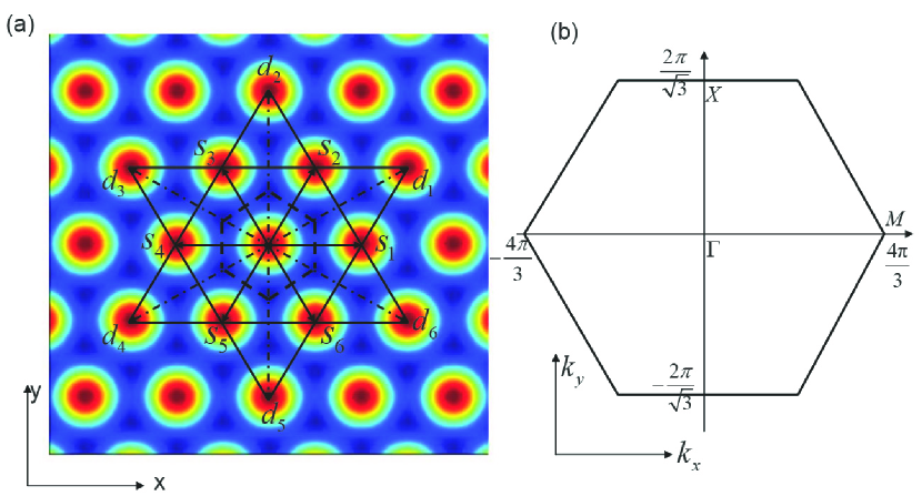
Figure 1: (Color online) (a). Uniform triangle lattices are formed from the maxima of the potential given by $V(\mathbf{r})=V_{L}\sum_{i=1}^{3}\cos(\mathbf{k}_{i}\cdot\mathbf{r})$. The defined lattice vectors $\mathbf{s}_{i}$ and $\mathbf{d}_{i}$ are shown. The hexangular zone encircled by the black-dashed lines is the unit cell of triangular lattice. (b) The Brillouin zone (BZ) of triangular lattices, and the high-symmetry points are marked.

Firstly, we apply three blue detuned laser beams to create two-dimensional TOLs, which can trap atoms at lattice sites. The three laser beams have same wave-vector length but different polarizations and are applied along three different directions: $\pm\frac{\sqrt{3}}{2}\hat{e}_{x}$ $-$ $\frac{1}{2}\hat{e}_{y}$ and $\hat{e}_{y}$, respectively. The total potential is given by $V(\mathbf{r})=V_{L}\sum_{i=1}^{3}\cos(\mathbf{k}_{i}\cdot\mathbf{r})$ with wave vectors $\mathbf{k}_{1,2}=k\left(\pm\frac{\sqrt{3}}{2},\frac{1}{2}\right)$ and $\mathbf{k}_{3}=k\left(0,1\right)$. The pattern of the potential is shown in Fig.1(a), where the maxima form perfect TOLs.

In order to simulate the RSOC, we consider the ultra-cold fermionic atoms trapped in the TOLs and having tripod-type level configuration (e.g., the lowest three Zeeman levels of ⁶Li atoms near the broad $s$-wave Feshbach resonance)Ruseckas ; Stanescu ; Zhu shown in Fig. 2(a). Three degenerate hyperfine ground states $|1\rangle$, $|2\rangle$ and $|3\rangle$ are coupled to an excited state $|4\rangle$ through spatially modulated two sets of lasers with the corresponding Rabi frequencies $\Omega_{v,1}$, $\Omega_{v,2}$ and $\Omega_{v,3}$ with $v=a,b$ denoting two independent sets. The Rabi frequencies can be parameterized as $\Omega_{v,1}=\frac{1}{2}\Omega_{v}\sin\theta_{v}\cos\phi_{v}e^{iS_{v,1}}$; $\Omega_{v,2}=\frac{1}{2}\Omega_{v}\sin\theta_{v}\sin\phi_{v}e^{iS_{v,2}}$; $\Omega_{v,3}=\frac{1}{2}\Omega_{v}\cos\theta_{v}e^{iS_{v,3}}$, and $\sum_{i=1}^{3}\left|\Omega_{v,i}\right|^{2}=\frac{1}{4}\Omega_{v}^{2}$. Thus, the system can be described by a Hamiltonian,

$$H_{0}=H_{tb}+H_{l-a}$$ (1)

with

$$H_{tb}=-\sum_{i,\alpha}\mu a_{i,\alpha}^{{\dagger}}a_{i,\alpha}-\sum_{i,j,\alpha,\beta}t_{i,j}a_{i,\alpha}^{{\dagger}}a_{j,\beta}$$ (2)

and

$$H_{l-a}=\underset{i,v}{\sum}\delta_{v}a_{i,4}^{{\dagger}}a_{i,4}-\underset{i,v,\alpha}{\sum}\hbar\Omega_{v,\alpha}a_{i,\alpha}^{{\dagger}}a_{i,4}+H.c$$ (3)

Here, $H_{tb}$ is the tight-binding Hamiltonian describing the atom hopping between different sites, and $H_{l-a}$ describes the laser-atom coupling. $\mu$ is the chemical potential. $a_{i,\alpha}^{{\dagger}}$ is the creation operator of atom on site $i$ and in state $|\alpha\rangle$ with $\alpha$=1, 2, 3. $t_{ij}$ is the hopping integral between site $i$ and $j$. $\delta_{v}$ is the detuning to the excited state $|4\rangle$.

Since the energy scale of $\delta_{v}$ and $\hbar\Omega_{v,\alpha}$ is much larger than that of $\mu$ and $t_{i,j}$ (See the below discussions about the parameters parts.), we firstly consider $H_{l-a}$. The eigenvalues of $H_{l-a}$ can be obtained from the diagonalization. Namely, $E_{i,v,n=1,2,3,4}=0,0,\frac{1}{2}(\delta_{v}\mp\sqrt{\delta_{v}^{2}+\hbar^{2}\Omega_{v}^{2}})$. The corresponding eigenstates (dressed states) are

$$|D_{i,v,1}\rangle =\sin\phi_{v}e^{iS_{v,3,1}}\left|1\right\rangle-\cos\phi_{v}e^{iS_{v,3,2}}\left|2\right\rangle$$

$$|D_{i,v,2}\rangle =\cos\theta_{v}\cos\phi_{v}e^{iS_{v,3,1}}\left|1\right\rangle+\cos\theta_{v}\sin\phi_{v}e^{iS_{v,3,2}}\left|2\right\rangle-\sin\theta_{v}\left|3\right\rangle$$

$$|B_{i,v,1}\rangle =\frac{1}{\sqrt{\Omega_{v}^{2}+(2E_{i,v,3})^{2}}}\left[\Omega_{v}\left(\sin\theta_{v}\cos\phi_{v}e^{iS_{v,3,1}}\left|1\right\rangle+\sin\theta_{v}\sin\phi_{v}e^{iS_{v,3,2}}\left|1\right\rangle+\cos\theta_{v}\left|3\right\rangle\right)-2E_{i,v,3}e^{iS_{v,3}}\left|4\right\rangle\right]$$

$$|B_{i,v,2}\rangle =\frac{1}{\sqrt{\Omega_{v}^{2}+(2E_{i,v,4})^{2}}}\left[\Omega_{v}\left(\sin\theta_{v}\cos\phi_{v}e^{iS_{v,3,1}}\left|1\right\rangle+\sin\theta_{v}\sin\phi_{v}e^{iS_{v,3,2}}\left|1\right\rangle+\cos\theta_{v}\left|3\right\rangle\right)-2E_{i,v,4}e^{iS_{v,3}}\left|4\right\rangle\right].$$ (4)

Here, $|B_{i,v,1/2}\rangle$ represent zero-energy dark states, while $|D_{i,v,1/2}\rangle$ represent the nonzero-energy bright states. That means the energy of dark states is not adjusted by the laser fields. Moreover, the dark states $|D_{i,v,1/2}\rangle$ have no coupling with the initial excited state $|4\rangle$. Therefore, the dark states are stable under atomic spontaneous emission. With the adiabatic approximationZhu ; Stanescu , we can neglect all the couplings that simultaneously involve the dark states and bright states and reduce the Hamiltonian $H_{0}$ into the subspace spanned by the dark states. In general, the dark states $|D_{i,a,1/2}\rangle$ produced by laser set $a$ (See the red lines in Fig. 2 (a)) are different from the dark states $|D_{i,b,1/2}\rangle$ produced by laser set $b$ (See the green lines in Fig. 2 (a)). However, the two sets of dark states can be same through initializing the parameters of the lasers, and the equivalence attributes to the periodicity of TOLs. In present work, we concentrate on the two sets of lasers configuration illustrated in Fig. 2 (b) and (c). The initialized parameters for the laser fields are $\theta_{a}=k_{a,2}y+\varphi$, $\phi_{a}=\frac{\pi}{4}$, $S_{a,1}=k_{a,1}x$, $S_{a,2}=-k_{a,1}x$, $S_{a,3}=k_{a,3}z$ and $\theta_{b}=k_{b,1}x+\varphi$, $\phi_{b}=k_{b,2}y+\frac{\pi}{4}$, $S_{b,1}=0$, $S_{b,2}=0$, $S_{b,3}=k_{b,3}z$, where $\varphi$ is an arbitrary phase and $k_{v,1}$, $k_{v,2}$ and $k_{v,3}$ are the wave vectors of the lasers along the $x$, $y$, $z$ axes, respectively. The wave vectors of the lasers are initialized to fulfil the relations: $k_{v,1}$=$4\pi$, $k_{v,2}$=$4\pi/\sqrt{3}$, so that the commensuration with the TOLs is guaranteed simultaneously. Now, $|D_{i,v,1}\rangle$=$\frac{\sqrt{2}}{2}(\left|1\right\rangle-\left|2\right\rangle)$, $|D_{i,v,2}\rangle$=$\frac{\sqrt{2}}{2}(\left|1\right\rangle+\left|2\right\rangle)\cos\varphi-\sin\varphi\left|3\right\rangle$ for both $v=a$ and $b$. That means the Hamiltonian (1) can be projected into the subspace spanned by $|D_{i,\uparrow}\rangle$ and $|D_{i,\downarrow}\rangle$ with $|D_{i,\uparrow}\rangle\equiv|D_{i,v,1}\rangle$ and $|D_{i,\downarrow}\rangle\equiv|D_{i,v,2}\rangle$ if the atoms are initially pumped to these dark states and they remain in the dark states. Here, we use $\sigma=\uparrow\downarrow$ to denote two pseudo-spin. Then, in the dark states subspace, the Hamiltonian $H_{0}$ can be projected into the following form:

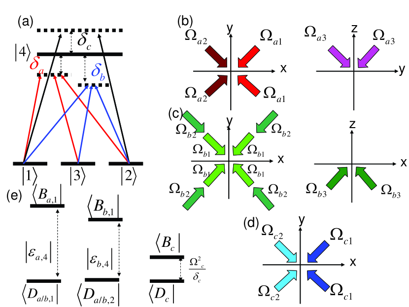
Figure 2: (color online) Illustration of the light-atom interaction for generation of effective non-Abelian gauge fields and effective Zeeman fields. (a) The configuration of the hyperfine levels of ultra-cold atom and three sets of laser beams characterized by the Rabi frequencies $\Omega_{a,i}$, $\Omega_{b,i}$ and $\Omega_{c,j}$ with $i=1,2,3$ and $j=1,2$. The atom and the laser fields have interaction through the Raman-type coupling with a large single-photon detuning $\delta_{a/b/c}$. The laser beams configuration for $\Omega_{a}$, $\Omega_{b}$ and $\Omega_{c}$ are shown in (b), (c) and (d). (e) The relative energy levels modulated by the atom-laser couplings.

$$H_{eff}=-\sum_{i,\sigma}\mu c_{i,\sigma}^{{\dagger}}c_{i,\sigma}-\sum_{i,j,\sigma,\sigma^{\prime}}t_{i,j}c_{i,\sigma}^{{\dagger}}U_{\sigma,\sigma^{\prime}i,j}c_{j,\sigma^{\prime}}\text{.}$$ (5)

Here, $c_{i,\sigma}^{{\dagger}}$ is the creation operator of atom on site $i$ in eigenstate $|D_{i,\uparrow}\rangle$. The Peierls phase factor is,

$$U_{\sigma,\sigma^{\prime}i,j}=U_{\sigma,\sigma^{\prime}i}U_{\sigma,\sigma^{\prime}j}^{{\dagger}}=e^{i\int_{\mathbf{r}_{j}}^{\mathbf{r}_{i}}(\mathbf{\tilde{A}}_{a.\sigma,\sigma^{\prime}}+\mathbf{\tilde{A}}_{b,\sigma,\sigma^{\prime}})\cdot d\mathbf{r}}$$ (6)

Where $\mathbf{\tilde{A}}_{v.\sigma,\sigma^{\prime}}$ is the laser-field-induced gauge vector potential, and $\mathbf{\tilde{A}}_{v,\sigma\sigma^{\prime}}$=$i\hbar\langle D_{v,\sigma}|\nabla|D_{v,\sigma^{\prime}}\rangle$. We list the forms of $\mathbf{\tilde{A}}_{v,\sigma\sigma^{\prime}}$ for completeness:

$$\mathbf{\tilde{A}}_{v,\uparrow\uparrow} =\hbar\left(\cos^{2}\phi_{v}\nabla S_{v,2,3}+\sin^{2}\phi_{v}\nabla S_{v,1,3}\right)$$

$$\mathbf{\tilde{A}}_{v,\uparrow\downarrow} =\hbar\cos\theta_{v}\left(\frac{1}{2}\sin 2\phi_{v}\nabla S_{v,1,2}-i\nabla\phi_{v}\right)$$

$$\mathbf{\tilde{A}}_{v,\downarrow\downarrow} =\hbar\cos^{2}\theta_{v}\left(\cos^{2}\phi_{v}\nabla S_{v,1,3}+\sin^{2}\phi_{v}\nabla S_{v,2,3}\right)$$ (7)

Note that since the two sets of lasers $a$ and $b$ have different detunings $\delta_{a}$ and $\delta_{b}$ to the excited state $|4\rangle$, there are no interference effects between the two sets, and they interact with the atoms independently. The total gauge vector potentials are the simple sum of $\mathbf{\tilde{A}}_{a.\sigma,\sigma^{\prime}}+\mathbf{\tilde{A}}_{b,\sigma,\sigma^{\prime}}$.

Now, we evaluate that the effective RSOC can be simulated by the aforementioned two sets of lasers $a$ and $b$. For convenience, we define the (next) nearest neighbor lattice vectors: $\mathbf{s}_{n}$ ($\mathbf{d}_{n}$) shown in Fig. 1 (a) with $n$=$1$…$6$, and set the lattice constant $1$. For the two sets of lasers configuration illustrated in Fig. 2 (b) and (c), we can find that $U_{\mathbf{s}_{1}}$=$U_{\mathbf{s}_{4}}^{{\dagger}}$=$e^{i4\pi\cos\varphi\sigma_{x}}$ and $U_{\mathbf{d}_{2}}$=$U_{\mathbf{d}_{5}}^{{\dagger}}$=$e^{i4\pi\cos\varphi\sigma_{y}}$ are the only nontrivial phase factors and other $U_{\mathbf{s}_{n}/\mathbf{d}_{n}}$ are trivial and equal $\mathbf{1}$. Since the TOLs have the rotation symmetry of point group $C_{3\upsilon}$, rotating the laser beams or the lattice systems with $\pm\frac{2\pi}{3}$ gives another two groups of nontrivial phase factors: $U_{\mathbf{s}_{3}}$=$U_{\mathbf{s}_{6}}^{{\dagger}}$=$e^{i4\pi\cos\varphi\sigma_{x}}$, $U_{\mathbf{d}_{1}}$=$U_{\mathbf{d}_{4}}^{{\dagger}}$=$e^{-i4\pi\cos\varphi\sigma_{y}}$ and $U_{\mathbf{s}_{2}}$=$U_{\mathbf{s}_{5}}^{{\dagger}}$=$e^{-i4\pi\cos\varphi\sigma_{x}}$, $U_{\mathbf{d}_{3}}$=$U_{\mathbf{d}_{6}}^{{\dagger}}$=$e^{-i4\pi\cos\varphi\sigma_{y}\text{ }}$, respectively. Here, $\sigma_{x/y}$ are the two Pauli matrix. For a two-component spin system, we have the following relation for the unitary operator:

$$U_{\sigma\sigma^{\prime}}=e^{i\alpha(\sigma_{x/y})_{\sigma\sigma^{\prime}}}=\cos\alpha+i(\sigma_{x/y})_{\sigma\sigma^{\prime}}\sin\alpha.$$ (8)

With Eq. (8), we can find that $H_{eff}$ in Eq. (5) has the form as follows,

$$H_{eff} =-\sum_{i,\sigma}\mu c_{i,\sigma}^{{\dagger}}c_{i,\sigma}-t\cos\alpha\sum_{i,,n,\sigma}c_{i,\sigma}^{{\dagger}}c_{i+\mathbf{s}_{n},\sigma}-t^{\prime}\cos\alpha\sum_{i,,n,\sigma}c_{i,\sigma}^{{\dagger}}c_{i+\mathbf{d}_{n},\sigma}$$

$$-it\sin\alpha\sum_{i,,n,\sigma,\sigma^{\prime}}(-1)^{n+1}c_{i,\sigma}^{{\dagger}}(\sigma_{x})_{\sigma\sigma^{\prime}}c_{i+\mathbf{s}_{n},\sigma^{\prime}}-it^{\prime}\sin\alpha\sum_{i,,n,\sigma,\sigma^{\prime}}(-1)^{n}c_{i,\sigma}^{{\dagger}}(\sigma_{y})_{\sigma\sigma^{\prime}}c_{i+\mathbf{d}_{n},\sigma^{\prime}}.$$ (9)

Here, $t$ and $t^{\prime}$ are the original nearest and next-nearest neighbor hopping integrals. $\alpha=4\pi\cos\varphi$. The first three terms in Eq. (9) are the modulated normal hopping parts of the Hamiltonian, while the last two terms describe the effective RSOC. More importantly, through adjusting the gauge flux $\alpha$, one can change the relative strength between the hopping and RSOC. That is nearly impossible in the condensed matter system. The $k^{3}$ type of RSOC can be explicitly found in the momentum space form of Eq. (9), which we will discuss in the next section.

In the following part of this section, we simulate how to generate an effective ZF to split two pseudo-spin states $|D_{i,\uparrow}\rangle$ and $|D_{i,\downarrow}\rangle$. We apply two additional laser beams that couple the states $\left|1\right\rangle$ and $\left|2\right\rangle$ to the excited state $\left|4\right\rangle$ with a large detuning $\delta_{c}$Zhu1 (See the blue lines in Fig. 2 (a) ). The laser-atom interaction is

$$H_{l-a}^{\prime}=-\underset{i}{\sum}\delta_{c}a_{i,4}^{{\dagger}}a_{i,4}+\underset{i,\alpha=1}{\overset{\alpha=2}{\sum}}\hbar\Omega_{c,\alpha}a_{i,\alpha}^{{\dagger}}a_{i,4}+H.c.$$ (10)

The corresponding Rabi frequencies are parameterized as $\Omega_{c,1}=\frac{\sqrt{2}}{4}\Omega_{c}e^{i4\pi x}$ and $\Omega_{c,2}=\frac{\sqrt{2}}{4}\Omega_{c}e^{-i4\pi x}$ with $\sqrt{\left|\Omega_{c,1}\right|^{2}+\left|\Omega_{c,2}\right|^{2}}=\frac{1}{2}\Omega_{c}$ and $\hbar\Omega_{c}\ll$ $\delta_{c}$. The lasers configuration is illustrated in Fig. 2 (d).

The eigenvalues of $H_{l-a}^{\prime}$ can be obtained from the diagonalization. Namely, $E_{i,n=1,2,3}^{\prime}=0,-\frac{1}{2}(\delta_{c}\mp\sqrt{\delta_{c}^{2}+\hbar^{2}\Omega_{c}^{2}})$. The corresponding eigenstates are:

$$\left|\chi_{1}\right\rangle =\frac{\sqrt{2}}{2}e^{-i4\pi x}\left|1\right\rangle-\frac{\sqrt{2}}{2}e^{i4\pi x}\left|2\right\rangle$$

$$\left|\chi_{2}\right\rangle =\frac{\sqrt{2}}{2}\cos\beta e^{-i4\pi x}\left|1\right\rangle+\frac{\sqrt{2}}{2}\cos\beta e^{i4\pi x}\left|2\right\rangle-\sin\beta\left|4\right\rangle$$

$$\left|\chi_{3}\right\rangle =\frac{\sqrt{2}}{2}\sin\beta e^{-i4\pi x}\left|1\right\rangle+\frac{\sqrt{2}}{2}\sin\beta e^{i4\pi x}\left|2\right\rangle+\cos\beta\left|4\right\rangle$$ (11)

Here, $\tan\beta=(\sqrt{\delta_{c}^{2}+\hbar^{2}\Omega_{c}^{2}}-\delta_{c})/\delta_{c}$. Due to $\hbar\Omega_{c}\ll$ $\delta_{c}$, we can get $\tan\beta\sim\hbar\Omega_{c}/\delta_{c}\sim 0$, and $E_{i,2}^{\prime}\sim\hbar^{2}\Omega_{c}^{2}/4\delta_{c}$.

$$\left|\chi_{2}\right\rangle\sim\frac{\sqrt{2}}{2}e^{-i4\pi x}\left|1\right\rangle+\frac{\sqrt{2}}{2}e^{i4\pi x}\left|2\right\rangle,\left|\chi_{3}\right\rangle\sim\left|4\right\rangle.$$ (12)

Since $E_{i,1}^{\prime}=0$, there is no effect of $\left|\chi_{1}\right\rangle$ to the ground states $\left|1\right\rangle$ and $\left|2\right\rangle$, and $\left|\chi_{4}\right\rangle$ also has no effect to $\left|1\right\rangle$ and $\left|2\right\rangle$. Hence, we can only consider the effect of $\left|\chi_{2}\right\rangle$ to $\left|1\right\rangle$ and $\left|2\right\rangle$. If we define that $d_{i}^{{\dagger}}$ is an operator to create an atom on site $i$ in eigenstate $\left|\chi_{2}\right\rangle$. A perturbation Hamiltonian can be written as: $H_{p}=$ $\hbar\Omega_{p}\sum_{i}d_{i}^{{\dagger}}d_{i}$. With Eq. (12), $H_{p}$ has the form:

$$H_{p}=H_{ac}+\hbar\Omega_{p}\underset{i}{\sum}e^{-i8\pi x}a_{i,1}^{{\dagger}}a_{i,2}+H.c.$$ (13)

Where $\Omega_{p}=$ $\hbar\Omega_{c}^{2}/8\delta_{c}$. $H_{ac}=$ $\hbar\Omega_{p}\underset{i}{\sum}(a_{i,1}^{{\dagger}}a_{i,1}+a_{i,2}^{{\dagger}}a_{i,2})$ is a constant ac-Stark shift, whose effect can be canceled with a frequency offset of the laser beams $\Omega_{v,3}$ applied to the level $\left|3\right\rangle$Zhu1 . Therefore, we can only consider the effect of the second term in Eq. (13). From Eq. (4), we can get the following relations

$$\left|1\right\rangle =\frac{\sqrt{2}}{2}\left(\left|D_{i,\uparrow}\right\rangle+\cos\varphi\left|D_{i,\downarrow}\right\rangle\right)$$

$$\left|2\right\rangle =\frac{\sqrt{2}}{2}\left(-\left|D_{i,\uparrow}\right\rangle+\cos\varphi\left|D_{i,\downarrow}\right\rangle\right)$$ (14)

Where we have applied the conditions that at all the lattice sites, $e^{\pm i8\pi x}=1$, $e^{\pm iS_{v,1,2}}=1$, $\theta=\varphi$ and $\phi=\pi/4$. With Eq. (14), we find the second term in Eq. (13) induce a splitting between $|D_{i,\uparrow}\rangle$ and $|D_{i,\downarrow}\rangle$ as:

$$H_{s} =-\hbar\Omega_{p}\underset{i}{\sum}(c_{i,\uparrow}^{{\dagger}}c_{i,\uparrow}-\cos^{2}\varphi c_{i,\downarrow}^{{\dagger}}c_{i,\downarrow})$$

$$=-h_{0}\underset{i,\sigma}{\sum}c_{i,\sigma}^{{\dagger}}c_{i,\sigma}-h_{z}\underset{i}{\sum}(c_{i,\uparrow}^{{\dagger}}c_{i,\uparrow}-c_{i,\downarrow}^{{\dagger}}c_{i,\downarrow}),$$

with $h_{0}=\hbar\Omega_{p}(1-\cos^{2}\varphi)/2$ and $h_{z}=\hbar\Omega_{p}(1+\cos^{2}\varphi)/2$. $h_{0}$ can be renormalized into the chemical potential term in $H_{eff}$ (Eq. (9)), and $h_{z}$ describes the effective ZF. In order to guarantee that $H_{s}$ cannot pump the atoms outside of the dark-state subspace, the conditions: $\hbar\Omega_{p}\ll\left|E_{b,3}\right|$ $<\left|E_{a,3}\right|$ must be fulfilled (See Fig. 2 (e)). Now, the new Hamiltonian including the effective RSOC and ZF is:

$$H_{0}^{\prime}=H_{eff}+H_{s}.$$ (15)

III Topological SF and Majorana Fermion

The SF states can be induced by atomic interaction from the s-wave scattering. The interaction term is described by the Hamiltonian:

$$H_{int}=\sum_{i}\sum_{\alpha<\beta}V_{\alpha\beta}a_{i,\alpha}^{{\dagger}}a_{i,\beta}^{{\dagger}}a_{i,\beta}a_{i,\alpha},$$ (16)

where $\alpha$ and $\beta$ label three ground states of atoms and $V_{\alpha\beta}$ are proportional to $s$-wave scattering lengths between $\alpha$, $\beta$ channel. In $s$-wave SF state, $H_{int}$ can be decoupled on the mean-field level:

$$H_{mf}=\sum_{i}\sum_{\alpha<\beta}\Delta_{\alpha\beta}a_{i,\alpha}^{{\dagger}}a_{i,\beta}^{{\dagger}}+H.c.$$ (17)

with $\Delta_{\alpha\beta}=V_{\alpha\beta}\left\langle a_{i,\beta}a_{i,\alpha}\right\rangle$, the SF order parameter. Under the condition of $\Delta_{\alpha\beta}\ll\Omega_{a/b}$, it is safe to consider the SF in the dark-state subspace, because $H_{mf}$ cannot pump the atoms outside of the dark-state subspace. Then, we project $H_{mf}$ to the dark-state subspace and have

$$H_{mf}^{\prime}=\sum_{i}\Delta_{0}c_{i,\uparrow}^{{\dagger}}c_{i,\downarrow}^{{\dagger}}+H.c.$$ (18)

with $\Delta_{0}$ the linear combinations of $\Delta_{\alpha\beta}$.

In the following parts of the paper, we focus on the total Hamiltonian which describes the SF states:

$$H_{t}=H_{0}^{\prime}+H_{mf}^{\prime}\text{.}$$ (19)

After the Fourier transformation, in momentum Nambu bases: $[c_{\mathbf{k\uparrow}},c_{\mathbf{k}\downarrow,}c_{-\mathbf{k\uparrow}}^{{\dagger}},c_{-\mathbf{k\downarrow}}^{{\dagger}},]^{T}$, $H_{t}$ can be expressed as:

$$H_{t}(\mathbf{k})=\left[\begin{array}[c]{cc}\varepsilon_{\mathbf{k}}-h_{z}\sigma_{z}+\mathbf{g}_{\mathbf{k}}\cdot\mathbf{\sigma}&-i\Delta_{0}\sigma_{y}\\ i\Delta_{0}\sigma_{y}&-(\varepsilon_{\mathbf{k}}-h_{z}\sigma_{z})+\mathbf{g}_{\mathbf{k}}\cdot\mathbf{\sigma}^{\ast}\end{array}\right].$$ (20)

Here $\mathbf{g}_{\mathbf{k}}=(a_{\mathbf{k}},b_{\mathbf{k}})$, $\mathbf{\sigma}=(\sigma_{x},\sigma_{y})$, and the explicit forms of $\varepsilon_{\mathbf{k}}$, $a_{\mathbf{k}}$ and $b_{\mathbf{k}}$ are listed:

$$\varepsilon_{\mathbf{k}} =-2t_{1}(\cos k_{x}+2\cos\frac{k_{x}}{2}\cos\frac{\sqrt{3}k_{y}}{2})$$

$$-2t_{3}(\cos\sqrt{3}k_{y}+2\cos\frac{3k_{x}}{2}\cos\frac{\sqrt{3}k_{y}}{2})-\mu^{\prime}$$ (21)

$$a_{\mathbf{k}} =2t_{2}(\sin k_{x}-2\sin\frac{k_{x}}{2}\cos\frac{\sqrt{3}k_{y}}{2})$$

$$b_{\mathbf{k}} =2t_{4}(-\sin\sqrt{3}k_{y}+2\sin\frac{\sqrt{3}k_{y}}{2}\cos\frac{3k_{x}}{2})$$ (22)

in which $t_{1}$=$t\cos\alpha$, $t_{2}$=$t\sin\alpha$, $t_{3}$=$t^{\prime}\cos\alpha$, $t_{4}$=$t^{\prime}\sin\alpha$ with $\alpha=4\pi\cos\varphi$ and $\mu^{\prime}=\mu+h_{0}$.

Before discussing the properties of the SF states described by $H_{t}$ in Eq. (19), we give the estimations about the parameters related to the aforementioned simulations to ensure the experimental feasibility and rationality. For trapped atoms: ⁶Li, the wave length of laser beams utilized to produce the TOL is $\lambda_{L}\sim 1\mu m$, and the lattice constant is $a_{L}=\frac{2\lambda_{L}}{\sqrt{3}}$. The recoil energy is $E_{r}=\frac{\hbar^{2}k_{L}^{2}}{2m}\sim\hbar\times 2\pi\times 30$ kHZ$\sim 1\mu K$ with $k_{L}=\frac{2\pi}{\lambda_{L}}$, and $t=\frac{4E_{r}}{\sqrt{\pi}}(\frac{V_{0}}{E_{r}})^{\frac{3}{4}}e^{-2\sqrt{V_{0}/E_{r}}}$Zwerger when $V_{0}>>$ $E_{r}$ with $V_{0}\sim 4V_{L}$, the depth of the TOL. $t^{\prime}/t=e^{-\eta(\sqrt{3}-1)\sqrt{(V_{0}-E_{kin})/E_{r}}k_{L}a_{L}}$ with $E_{kin}$ and $\eta$ the kinetic energy of atom and the renormalized factor. The typical atomic velocity is about several centimeters per second, and $E_{kin}$ has the same order of $E_{r}$. $\eta$ depends on geometry of the lattice. According to the 1D lattice resultsBloch and $\eta<1$, we estimate that $V_{0}\sim 3E_{r}$ is enough to get $t^{\prime}/t=\frac{1}{3\sqrt{3}}$. Actually, the TSF is robust even when $t^{\prime}/t\sim 10^{-3}$. Here, without lost of generality, we set $t^{\prime}/t\equiv\frac{1}{3\sqrt{3}}$. Then $t\sim 0.1E_{r}$ with the aforementioned formula. From the harmonic-potential approximation, the energies of the atoms tightly confined at a single lattice site are quantized to levels separated by $2\pi\hbar\omega_{0}$=$2E_{r}\sqrt{\frac{V_{0}}{E_{r}}}$Bloch . On the other hand, the maximal band width for the TOL is $W_{m}\sim 10t$ $\sim E_{r}$. Therefore, it is safe to describe the system with single-band approximation because of $2\pi\hbar\omega_{0}>W_{m}$. The Rabi frequencies $\Omega_{a/b/c}$ are $10^{3}E_{r}/\hbar$, and the $\Omega_{p}$ can be tuned from $0$ to $E_{r}/\hbar$ which is enough for $\hbar\Omega_{p}\ll\left|E_{b,3}\right|$ $<\left|E_{a,3}\right|$. Then, adiabatic approximationZhu1 is reasonable. The typical $s$-wave pairing potential $\Delta_{\alpha\beta}$ in experiments is about $0.1E_{r}/\hbar$Ketterle , which is much smaller than $\Omega_{a/b}$. Hence, our proposal is experimentally feasible when the parameters lie in the estimated region.

For convenience to discuss the properties of SF, we rewrite $H_{t}(\mathbf{k})$ in the new bases $[\hat{\psi}_{\mathbf{k,}+},\hat{\psi}_{-\mathbf{k,}+}^{{\dagger}},-\hat{\psi}_{-\mathbf{k,}-}^{{\dagger}},-\hat{\psi}_{\mathbf{k,}-}]^{T}$ with $\hat{\psi}_{\mathbf{k,}\pm}$= $\frac{1}{\sqrt{2}}\left[c_{\mathbf{k\uparrow}}\pm c_{-\mathbf{k\downarrow}}^{{\dagger}}\right]$, $H_{t}^{\prime}$ has the following form:

$$H_{t}^{\prime}(\mathbf{k})=\left[\begin{array}[c]{cc}H_{+}(\mathbf{k})&-i\varepsilon_{\mathbf{k}}\sigma_{y}\\ i\varepsilon_{\mathbf{k}}\sigma_{y}&H_{-}(\mathbf{k})\end{array}\right].$$ (23)

Here,

$$H_{\pm}(\mathbf{k})=\pm\left[(-h_{z}\mp\Delta_{0})\sigma_{z}+a_{k}\sigma_{x}\pm b_{k}\sigma_{y}\right].$$ (24)

The spectrums of Hamiltonian(23) are $\pm E_{\pm}(k)$, and

$$E_{\pm}(k)=\sqrt{\varepsilon_{\mathbf{k}}^{2}+\Delta_{0}^{2}+\Theta_{k}^{2}\pm 2\sqrt{h_{z}^{2}\Delta_{0}^{2}+\varepsilon_{\mathbf{k}}^{2}\Theta_{k}^{2}}},$$ (25)

in which $\Theta_{k}=\sqrt{h_{z}^{2}+\left|\mathbf{g}_{\mathbf{k}}\right|^{2}}$. The topological transition point is determined by bulk energy gap closing condition: $E_{-}(k)=0$ (Fig. 3(d)). The spectrums are fully gapped off this point, and the SF is topologically nontrivial when $h_{z}>\sqrt{\Delta_{0}^{2}+\varepsilon_{\mathbf{k}}^{2}}|_{\mathbf{k}=(0,0)}$ (Fig. 3(c)) and trivial when $h_{z}<\sqrt{\Delta_{0}^{2}+\varepsilon_{\mathbf{k}}^{2}}|_{\mathbf{k}=(0,0)}$ (Fig. 3(e)). Around the $\Gamma$ point in BZ,

$$\mathcal{H}_{\pm}(\mathbf{k})=\mp[(\Delta_{0}\pm h_{z})\sigma_{z}+\lambda_{so}(k_{-}^{3}\sigma_{\pm}+k_{+}^{3}\sigma_{\mp})]\text{,}$$ (26)

where $\sigma_{\pm}$=$\frac{1}{2}\left(\sigma_{x}\pm\sigma_{y}\right)$, $k_{\pm}$=$\frac{1}{2}\left(k_{x}\pm k_{y}\right)$. The term $\lambda_{so}(k_{-}^{3}\sigma_{\pm}+k_{+}^{3}\sigma_{\mp})$ is the $k^{3}$ RSOC with amplitude: $\lambda_{so}$=$\frac{t_{2}}{2}\sim-0.48t$ for $\cos\varphi=-0.101$. It is explicit that $\mathcal{H}_{\pm}(\mathbf{k})$ has the well-defined $f$-wave chirality. That means the topological Chern numberThouless can be calculated $\mathcal{C}_{\mathcal{H}_{-}}$=$\frac{3}{2}\left[\text{sign}(h_{z}-\Delta_{0})_{h_{z}>\Delta_{0}}-\text{sign}(h_{z}-\Delta_{0})_{h_{z}<\Delta_{0}}\right]$=$3$ while $\mathcal{C}_{\mathcal{H}+}$=$0$. From the square lattice results that $\Delta_{0}$ has maximum when the filling $\sim$ 1 atom per siteHofstetter , we set $\Delta_{0}=0.5t$ and $\hbar\Omega_{p}=3\Delta_{0}$ for the chemical potential around $\mu_{1}$ and filling about 0.6 atom per site. When the chemical potential locates at the region of $\mu_{4}$ (Fig. 3 (b)), the low-energy behaviors are dominated by $H_{t}^{\prime}(\mathbf{k})$ with $\mathbf{k}\sim(0,\frac{2\sqrt{3}\pi}{3})$. Then we cannot define the specific chirality, and we ascribe these cases to NSF. According to the aforementioned analysis, we draw the phase diagram in Fig. 3(e). We find that the TSF strongly depends on the initial parameter $\varphi$ of the laser beams and the fillings. That means we can control the topological properties of the SF by modulating the parameters of the lasers. That provides convenience to investigate the TSF.

In lattice case, the ground state Chern number of $H_{t}$ can be calculated with:

$$\mathcal{C}_{n}=\frac{1}{2\pi}\int_{BZ}d^{2}k2Im\langle\frac{\partial u_{n}(\mathbf{k})}{\partial k_{x}}|\frac{\partial u_{n}(\mathbf{k})}{\partial k_{y}}\rangle,$$ (27)

where $u_{n}(\mathbf{k})$ is the ground state wave-function for the $n$th occupied band ($n$=1,2). The straightforward calculation gives $\mathcal{C}_{1}$=$0$ and $\mathcal{C}_{2}$=$3$ when $h_{z}>\sqrt{\Delta_{0}^{2}+\varepsilon_{\mathbf{k}}^{2}}|_{\mathbf{k}=(0,0)}$, and $\mathcal{C}_{1}$=$0$ and $\mathcal{C}_{2}$=$0$ when $h_{z}<\sqrt{\Delta_{0}^{2}+\varepsilon_{\mathbf{k}}^{2}}|_{\mathbf{k}=(0,0)}$. The non-zero Chern number means the same numbers of gapless edge states from the bulk-edge correspondence. From the energy spectrum of $H_{t}(k_{y},x)$ shown in Fig. 4, we find that three gapless chiral edge states transport on one edge of TSF. (see Fig.4 (a) and (d)). The effective Hamiltonian describing the chiral edge states is

$$\mathcal{H}_{edge}=\sum_{k_{y}\geq 0}\nu_{0}k_{y}\hat{\Psi}_{k_{y}}^{{\dagger}}(x)\hat{\Psi}_{k_{y}}(x),$$ (28)

where $\nu_{0}$ is the effective velocity at $\Gamma$, and $\hat{\Psi}_{k_{y}}^{{\dagger}}(x)=\sum_{\sigma}\int dx\left[u_{k_{y},\sigma}(x)c_{\sigma}^{{\dagger}}(x)+v_{k_{y},\sigma}(x)c_{\sigma}(x)\right]$. The Majorana condition requires $\hat{\Psi}_{-k_{y}}(x)=$ $\hat{\Psi}_{k_{y}}^{{\dagger}}(x)$, i.e., $u_{-k_{y,\sigma}}(x)=v_{k_{y,\sigma}}^{\ast}(x)$. We check that it’s indeed the case in our model. That means three edge states are chiral Majorana edge states.

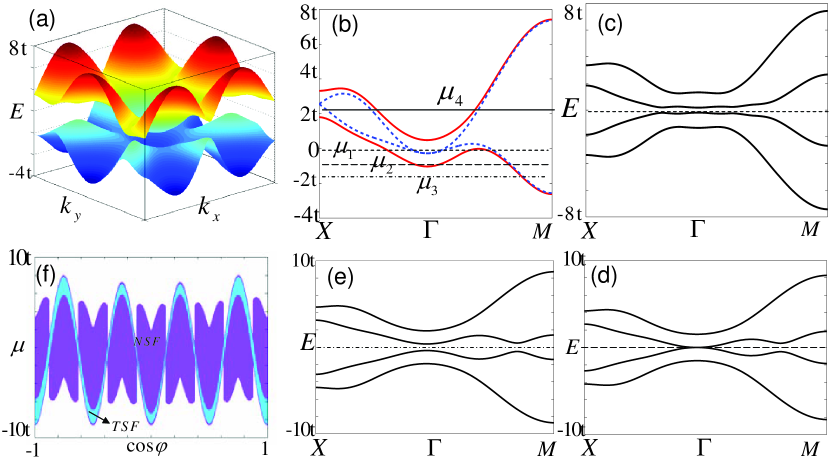
Figure 3: (color online) (a) The band structures of $E_{k}=\varepsilon_{k}\pm\Theta_{k}$ with $\cos\varphi=-0.101$ and $\mu=-2.59$. Here, we set $k_{x}\in[-\frac{4\pi}{3},\frac{4\pi}{3}]$ and $k_{y}\in[-\frac{2\pi}{\sqrt{3}},\frac{2\pi}{\sqrt{3}}]$. (b) The band structures along high symmetric lines (Fig.2 (b)). The dashed blue lines are $\varepsilon_{k}\pm\left|g_{k}\right|$ and the solid red lines correspond to (a). Four different fillings with chemical potential $\mu_{1/2/3/4}=-2.59t$, $-3.436t$, $-3.89t$, $0.45t$ are shown. (c) (d) (e) are the SF quasi-particle spectrums corresponding to $\mu_{1}$, $\mu_{2}$ and $\mu_{3}$. (f) The phase diagram as change of $\cos\varphi$ and $\mu$. Two different phases, NSF and TSF are identified. $\Delta_{0}=0.5t$ and $\hbar\Omega_{p}=3\Delta_{0}$.

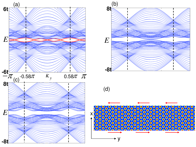
Figure 4: (color online) The spectrums of Hamiltonian (19) with edges at x direction $i_{x}$ $\in(1,31)$. (a) (b) and (c) correspond to $\mu_{1}$ $\mu_{2}$ and $\mu_{3}$ cases in Fig. 3 (b). The dashed black lines indicate the contributions from the first BZ. (d) The edge states (the states crossing the gap and denoted with the solid red lines in (a)) transport along two edges.

In general, the topological defects bound Majorana zero modes in TSC/TSFQi ; Read . Here, we consider the topological excitations of vortex structures in our system. The quasi-particle excitations usually are described by the Bogoliubov-de Gennes (BdG) equation. From Fig. 4(a), we can find that the wave function of low energy excitations can be constructed from the contributions of quasi-particle around $\Gamma$. For simplicity, only the non-trivial part $\mathcal{H}_{-}(k)$ of Eq.(26) is taken into account. Define $z=x+iy$, then $\partial_{z/z^{\ast}}=\partial_{x}\pm i\partial_{y}$. The BdG equation for the quasi-particle has the form: $\mathcal{H}_{-}(z,z^{\ast})\Psi_{0}=E\Psi_{0}$ with $\Psi_{0}=[u_{0}^{\ast},v_{0}^{\ast}]^{T}$ and the corresponding quasi-particle creation operator: $\hat{\Psi}_{0}^{{\dagger}}={\displaystyle\int}dzdz^{\ast}\left[u_{0}\hat{\psi}_{-}^{{\dagger}}+v_{0}\hat{\psi}_{-}\right]$. In the uniform TSF states, we can assume a trivial wave function: $u_{0}=e^{i\pi/4}z^{-\frac{3}{2}}e^{-\frac{2}{3}(\frac{h_{z}-\Delta_{0}}{\lambda_{so}})^{1/3}(zz^{\ast})^{\frac{3}{2}}}$ and $v_{0}=u_{0}^{\ast}$ as a test wave function from the BdG equation. The SF order parameter with a vortex structure can be approximately expressed as $\Delta_{0}(r)$=$0$ for $r<r_{c}$ and $\Delta_{0}(r)$=$\Delta_{0}e^{i\theta}$ for $r>r_{c}$ with vorticity $1$. We imagine that the vortex is created adiabatically by changing the wave function slowly enough so that it always remains an eigenstate. The wave function of the vortex state can be obtained from a singular gauge transformation: $\Psi_{0}\rightarrow\Psi_{0}e^{iq\theta}$ with $q=\pm 1$ identifying the quasi-particle and quasi-anti-particle. In reverse, the vortex can be gauged away by the inverse singular gauge transformation: $k\rightarrow k-\nabla\theta/2$ and $\Delta_{0}e^{i\theta}\rightarrow\Delta_{0}$ Sato2 . After the inverse transformation, the state is one of eigenstates, namely, the vortex excited state. In analogy to the Laughlin’s argumentLaughlin about the vortex excitation in quantum Hall state, we get the wave function describing vortex zero mode as $u_{0}^{\prime}\sim e^{-i(\frac{\theta}{2}-\frac{\pi}{4})}r^{-\frac{3}{2}}e^{-\frac{2}{3}\left(\frac{h_{z}-\Delta_{0}}{\lambda_{so}}\right)^{\frac{1}{3}}r^{3}}$ and $v_{0}^{\prime}=(u_{0}^{\prime})^{\ast}$. The unique one zero mode for $f$-wave case is proven by the numerical calculationMao .

The stability of Majorana zero mode is measured by the mini-gap $E_{g}\sim\Delta_{0}^{2}/E_{f}$ with $E_{f}$ the Fermi energy. In our case, the $E_{f}$ is measured by $t$ not $E_{kin}$. Hence, The ratio $E_{g}/\Delta_{0}$ can be large enough to protect Majorana zero mode. Take half filling as an example, we assume the optimized $\Delta_{0}\sim t$ and roughly estimate $E_{f}\sim$ $3t$. Then $E_{g}/\Delta_{0}\sim 1/3$. Comparing with the hybridized systems Fu ; Sau ; Mao , the energy scale of $E_{f}$ has the order of electrons’ kinetic energy $E_{kin}$ and $\Delta_{0}$ from the proximity effect is much smaller compared to $E_{kin}$. So, the mini-gap in hybridized systems may be relative small compare to superconductive gap $\Delta_{0}$.

IV
Conclusions

In summary, we have proposed a scheme to produce $k^{3}$ RSOC and ZF through the laser-atom interaction in TOLs, and a novelly chiral $f$-wave TSF is realized thanks to the $s$-wave Feshbach resonance. We find that there exists three Majorana edge states locating on the boundary of the system and one Majorana fermion bounding to each vortex in the TSF state. The TSF can be controlled by modulating the parameters of the laser. The controllability provides convenience to investigate the properties of the TSF. Our proposal enlarges TSF family and presents some advantages to study the Majorana fermions.

Acknowledgments: Ningning Hao thanks J. Li and Guocai Liu thanks S. L. Zhu for helpful discussions. The work is supported by the Ministry of Science and Technology of China 973 program(2012CB821400), NSFC-1190024, NSFC-11147171 and NSFC-11247011.

References

• (1) X. Qi, T. L. Hughes, S. Raghu, and S. Zhang, Phys. Rev. Lett. 102, 187001 (2009).
• (2) X. Qi and S. Zhang, Rev. Mod. Phys. 83, 1057 (2011).
• (3) C Nayak, S. H. Simon, A. Stern, M. Freedman and S. D. Sarma, Rev. Mod. Phys. 80, 1083 (2008).
• (4) D. D. Osheroff, Rev. Mod. Phys. 69, 667 (1997).
• (5) A. P. Mackenzie and Y. Maeno, Rev. Mod. Phys. 75, 657 (2003).
• (6) L. Fu and C. L. Kane, Phys. Rev. Lett. 100, 096407 (2008).
• (7) J. D. Sau, R. M. Lutchyn, S. Tewari and S. D. Sarma, Phys. Rev. Lett. 104, 040502 (2010).
• (8) L. Mao, J. Shi, Q. Niu and C. Zhang1, Phys. Rev. Lett. 106, 157003 (2011).
• (9) X. Qi, T. L. Hughes, and S. Zhang, Phys. Rev. B 82, 184516 (2010).
• (10) S. B. Chung, H. Zhang, X. Qi, and S. Zhang, Phys. Rev. B 84, 060510 (2011).
• (11) V. Mourik, K. Zuo, S. M. Frolov, S. R. Plissard, E. P. A. M. Bakkers and L. P. Kouwenhoven, Science 336, 1003 (2012).
• (12) S. Zhu, H. Fu, C. Wu, S. Zhang, and L. Duan, Phys. Rev. Lett. 97, 240401 (2006).
• (13) M. Sato, Y. Takahashi, and S. Fujimoto, Phys. Rev. Lett. 103, 020401 (2009).
• (14) L. Shao, S Zhu, L. Sheng, D. Xing, and Z. Wang, Phys. Rev. Lett. 101, 246810 (2008).
• (15) C. Zhang, S. Tewari, R. M. Lutchyn and S. D. Sarma, Phys. Rev. Lett. 101, 160401 (2008).
• (16) C. Zhang, Phys. Rev. A. 82, 021607(R) (2010).
• (17) K. Osterloh, M. Baig, L. Santos, P. Zoller and M. Lewenstein, Phys. Rev. Lett. 95, 010403 (2005).
• (18) J. Ruseckas G. JuzeliΕ«nas, P. Γ–hberg, and M. Fleischhauer, Phys. Rev. Lett. 95, 010404 (2005).
• (19) P. Wang, Z. Yu, Z. Fu, J. Miao, L. Huang, S. Chai, H. Zhai, and J. Zhang, Phys. Rev. Lett. 109, 095301 (2012).
• (20) L. W. Cheuk, A. T. Sommer, Z. Hadzibabic, T. Yefsah, W. S. Bakr, and M. W. Zwierlein, Phys. Rev. Lett. 109, 095302 (2012).
• (21) J. Struck, C. Γ–lschlΓ€ger, M. Weinberg, P. Hauke, J. Simonet, A. Eckardt, M. Lewenstein, K. Sengstock, and P. Windpassinger, Phys. Rev. Lett. 108, 225304 (2012).
• (22) P. Hauke, O. Tieleman, A. Celi, C. Γ–lschlΓ€ger, J. Simonet, J. Struck, M. Weinberg, P. Windpassinger, K. Sengstock, M. Lewenstein, and A. Eckardt, Phys. Rev. Lett. 109, 145301 (2012).
• (23) O. Tieleman, O. Dutta, M. Lewenstein, and A. Eckardt, Phys. Rev. Lett. 110, 096405 (2013).
• (24) E. I. Rashba. Sov. Phys. Solid State 2, 1109 (1960).
• (25) J. K. Chin, D. E. Miller, Y. Liu, C. Stan, W. Setiawan, C. Sanner, K. Xu and W. Ketterle, Nature (London) 443, 961 (2006).
• (26) M. Sato and S. Fujimoto, Phys. Rev. B 79, 094504 (2009).
• (27) H. Hung, W. Lee, C. Wu, Phys. Rev. B 83, 144506 (2011);W. Lee, C. Wu, and S. D. Sarma, Phys. Rev. A 82, 053611 (2010).
• (28) T. D. Stanescu, C. Zhang, and V. Galitski, Phys. Rev. Lett. 99, 110403 (2007).
• (29) S. Zhu, L.-B. Shao, Z. D. Wang, and L.-M. Duan, Phys. Rev. Lett. 106, 100404 (2011).
• (30) W. Zwerger, Journal of Optics B: Quantum and Semiclassical Optics 5, 9 (2003).
• (31) I. Bloch, J. Dalibard and W. Zwerger, Rev. Mod. Phys, 80, 885 (2008).
• (32) W. Ketterle and M.W. Zwierlein, Riv. Nuovo Cimento Soc. Ital. Fis. 31, 247 (2008).
• (33) D. J. Thouless, M. Kohmoto, M. P. Nightingale and M. den Nijs, Phys. Rev. Lett. 49, 405 (1982).
• (34) W. Hofstetter, J. I. Cirac, P. Zoller, E. Demler, and M. D. Lukin, Phys. Rev. Lett. 89, 220407 (2002).
• (35) N. Read and D. Green, Phys. Rev. B 61, 10267 (2000).
• (36) M. Sato, Y. Takahashi and S. Fujimoto, Phys. Rev. B, 82, 134521 (2010).
• (37) R. B. Laughlin, Phys. Rev. Lett. 50, 1395 (1983).