A non-LTE modeling of narrow emission components of He and Ca lines in optical spectra of CTTS

Keywords: stars – individual: GM Aur, BP Tau, DK Tau, DN Tau, GI Tau, GK Tau, V836 Tau, DI Cep, TW Hya – T Tauri stars – stellar atmospheres – radiative transfer – spectra.

Abstract

A spectrum of a hot spot, produced by radiation of accretion shock at T Tauri star’s surface, has been calculated taking into account non-LTE effects for He I, He II, Ca I and Ca II, using LTE-calculations of spot’s atmospheric structure, calculated by Dodin & Lamzin (2012). Assuming that pre-shock gas number density $N_{0}$ and its velocity $V_{0}$ are the same across the accretion column, we calculated spectra of a system ”star + round spot” for a set of $N_{0},$ $V_{0}$ values and parameters, which characterized the star and the spot.

It has been shown that theoretical spectra with an appropriate choice of the parameters reproduce well observed veiling of photospheric absorption lines in optical band as well as profiles and intensities of so-called narrow components of He II and Ca I emission lines in spectra of 9 stars. We found that accreted gas density $N_{0}>10^{12}$ cm^-3 for all considered stars except DK Tau. Observed spectra of 8 stars were succesfully fitted, asuming solar abundance of calcium, but it appeared possible to fit TW Hya spectrum only under assumption that calcium abundance in accreted gas was three times less than solar. We derive spot’s parameters by comparison of theoretical and observed spectra normalised to continuum level, so our results are independent on unknown value of interstellar extinction.

We have found that the predicted flux in Ca II lines is less than observed one, but this discrepancy can be resolved if not only high-density but also lower density gas falls onto the star. Theoretical equivalent widths as well as relative intensities of He I subordinate lines disagree significantly with observations, presumbly due to a number of reasons: necessity to take into account non-LTE thermal structure of upper layers of a hot spot, poorly known collisional atomic data for He I upper levels and inhomogeneity of the hot spot.

Introduction

Classical T Tauri stars (CTTS) are young (the age $<10^{7}$ yr), low mass $(M\leq 3\,M_{\odot})$ pre-main sequence stars, activity of which is caused by magnetospheric accretion of matter from a protoplanetary disc. An optical spectrum of CTTS consists of photospheric spectrum of late type star and emission lines with non-trivial and variable profiles. Generally speaking, CTTS’s emission lines consist of two components: a narrow ($FWHM\sim 30$ km s^-1) and a broad $(FWHM>100$ km s^-1), which are formed in different spatial regions – see e.g. Batalha et al. (1996), Dodin et al. (2012). Flux ratio of these components is different for different lines, varies from star to star and with time for the same line.

It has been known since Joy (1949) that depths and equivalent widths of photospheric lines in T Tauri stars spectra are smaller than those of main-sequence stars of the same spectral type. This effect is used to explain as the result of superposition of continuum emission onto photospheric spectrum. The degree of veiling of CTTS’s photospheric absorption lines in some spectral band can be characterized by value

$$r={EW_{0}\over EW}-1,$$ (1)

averaged over lines of that regin, where $EW$ and $EW_{0}$ are equivalent widths of photospheric lines in spectra of CTTS and template star of the same spectral type respectively.

Line and continuum emission observed in CTTS’s spectra can be explained as follows in the frame of magnetospheric accretion model (Königl, 1991; Lamzin, 1995). The matter from the inner disk is frozen in the stellar magnetic field lines and slides down along them toward the star, being accelerated by gravity. Having reached the dense layers of the stellar atmosphere, matter is decelerated in the accretion shock (AS), converting into the heat the main part of its kinetic energy, the flux of which is equal to

$$F_{ac}={\mu m_{p}N_{0}V_{0}^{3}\over 2},$$ (2)

where $N_{0}$, $V_{0}$ are pre-shock gas number density and velocity, $\mu=1.3$ is the average molecular weight, $m_{p}$ is the proton mass. The hot postshock matter cools down gradually radiating its thermal energy in the UV and X-ray spectral bands and settles down to the stellar surface.

One half of the short-wavelength radiation flux of the shock from the cooling zone irradiates the star, producing so-called hot spot on its surface, and the second half escapes upward, heating and ionizing the pre-shock gas. Calculations show, that pre-shock gas temperature does not exceed 20 000 K at a typical velocity $V_{0}\sim 300$ km s^-1, however there are ions up to O⁺⁵ in this region (Lamzin, 1998).

Assuming that CTTS’s emission continuum is formed in the hot spot, Calvet and Gullbring (1998) have calculated the structure of the atmosphere being irradiated by the short-wave radiation of the accretion shock without any allowance for the emission in lines. However it was discovered later that photospheric lines in spectra of some CTTSs were filled in by the narrow emission lines (Petrov et al., 2001; Gham et al., 2008; Petrov et al., 2011), which were apparently formed in the hot spot and which in addition to continuum reduce the depth of a photospheric lines. This phenomenon leads for example to a variability of the radial velocity of photospheric lines and/or to a non-monotonic spectral energy distribution (SED) of the veiling continuum (Stempels and Piskunov, 2003), if to derive it by means of Eq.(1).

The calculations of the thermal structure and SED of the hot spot with allowance for the lines as well as the continuum for the first time have been performed by Dodin and Lamzin (2012) in LTE-approach. The calculations were performed for various sets of a parameters characterizing the star ($T_{ef},$ $\log\,g$) and an accretion shock ($N_{0},$ $V_{0}$) with solar element abundance.

It was assumed that there was one circular spot at stellar surface, within which $V_{0}$ and $N_{0}$ were constant. We calculated how the resulting spectra of a star with $T_{ef}$ from 3750 to 5000 K $+$ a spot should looks like at different relative sizes of the spot $f$ and its positions relative to the Earth, characterized by the angle $\alpha$ between the line of sight and spot’s axis of symmetry. For each of the stars in which veiling by lines was found (Gahm et al. 2008; Petrov et al. 2011), we were able to select a model with a spectrum similar to the observed one, at least in the sense that the lines exhibiting an emission feature in the observed spectra also exhibit emission features in the models. Thus, it was shown that the most strong emission lines being formed in the spot appeared in the spectra of CTTS as narrow components of emission lines, while more weak emission lines decreased the depth of respective photospheric lines.

However a quantitative comparison of simulated and observed spectra revealed a number of problems: there were not emission lines in some CTTS’s spectra predicted by the models; theoretical spectra did not reproduce observed intensity ratio of He I and He II lines; the predicted intensity of Ca I emission lines was so much greater than observed that Dodin and Lamzin (2012) suggested a substantial depletion of Ca in the accreted gas. However, the authors supposed that assumptions taken in the modeling were more probable reason of the discrepancy. First of all it is LTE-approach, because, as noted Sakhibullin (1997), the intensity of emission lines is usually smaller in non-LTE spectra.

It will be shown below that if to derive level populations and ionization degree of He and Ca from statistical equilibrium equations instead of Boltzmann and Saha equations, then the agreement between the theory and observations becames much better for a number of cases.

We, as well as Dodin and Lamzin (2012), consider only narrow components of emission lines, which are formed in the post-shock zone, where a problem of radiative transfer can be treated in the plane-parallel approximation. Broad components of CTTS’s emission lines in one way or another are formed in several regions: in the pre-shock H II zone, in the region near truncation radius, where disk matter is freezes in magnetic field lines of the star as well as in CTTS’s outflow. Hydrogen lines are example of the lines, in which the broad component usually dominates. A simulation of an intensity and profiles of emission lines broad component is much more complicated problem, which suggests simultaneous solution of 3-D MHD equations and 3-D radiative transfer – see, for instance, Kurosawa and Romanova (2012) and references therein.

1 The method of non-LTE calculations of He I and He II level populations

The software for the calculations of helium ionization degree and level populations was developed by ourself. The selection of atomic levels (so-called the atomic model) that we used in our calculations is described in the Appendix.

The region behind the shock front can be divided into two regions for convenience: the post-shock cooling zone, which is transparent to X-ray and ultraviolet radiations of the cooling gas, and the hot spot, i.e. the stellar atmosphere, where this radiation is absorbed. Distributions of the temperature $T$ and the number density over the post-shock cooling zone were taken from Lamzin’s paper (1998) for the parameters $V_{0}=200-400$ km s^-1 and $\log\,N_{0}=11.5-13.0.$ The distributions of the same parameters in the hot spot for the same values of $V_{0},$ $N_{0}$ and for various parameters of an undisturbed atmosphere of the star were calculated by Dodin and Lamzin (2012).

The spectrum of the hot spot is mainly determined by the parameter $K$ (Calvet and Gullbring, 1998; Dodin and Lamzin, 2012), which equals to the ratio of the flux $F_{ac}$ of the accretion energy – see Eq.(2) – to the stellar flux:

$$K=\frac{1}{2}{F_{ac}\over\sigma T_{ef}^{4}}.$$

The distributions of $T,$ $N,$ and He⁺ ion relative abundance as well as the populations of the levels with the principal quantum number $n=3$ and $n=4$ for two models with a difference in $K$ about 25 times are shown in Fig 1.

The choice of the ion and the principal quantum numbers for the figure is due to the fact that He II 4686 Å line will be actively used to determine accretion flow parameters. In order to display on the figure only the regions with a noticeable abundance of He II, we use a logarithm of He II 304 line’s optical depth normalized to its maximum value as the abscissa.

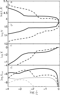
Figure 1: The distribution of the parameters in the formation region of the He II lines for a star with $T_{ef}=4000$ K and $\log g=4.0:$ the temperature (a), the number density (b), the relative abundance of He⁺ (c), the relative abundance of the levels of He II with $n=3$ (d, thick lines) and $n=4$ (d, thin lines). The solid lines correspond to the model with $V_{0}=400$ km s^-1, $\log N_{0}=12.5$ ($K=7.6$), the dash-dotted line corresponds to the model with $V_{0}=200$ km s^-1, $\log N_{0}=12$ ($K=0.3$). $\tau$ is the optical depth of the line at $304$ Å with the maximum value $\tau_{0},$ which correspondingly equals to $3.0\times 10^{4}$ and $1.0\times 10^{4}$.

The system of equations describing a balance of the level populations in a multilevel atom in stationary conditions is well known (see, for instance, Mihalas, 1978; Sakhibullin, 1997) and it is useless to write it here. We will describe only which atomic data were used and how the system of equations was solved.

The Einstein coefficients and the oscillator strengths for all (213 in total) transitions in our atomic model of He I were taken from the NORAD database (Nahar, 2010). The same values for He⁺ ion were calculated by means of formulae adopted from the textbook of Berestetskij et al. (1989). He I recombination coefficients were taken from the NORAD database, and the same for He II – from the Cloudy08 program (Ferland et al., 1998). The photoionization cross section for each level of He I was taken from the NORAD database, and for He II it was calculated according to Golovatyj et al. (1997).

The rate coefficients for electron impact excitation and de-excitation for He I and He II were calculated by means of data from the CHIANTI v.5.0 database (Dere et al., 1997; Landi et al., 2006) for each transition from $n=1,$ 2 levels to levels with $n\leqslant 5$. The impact rate coefficient for the $n=3\rightarrow 4$ transition of He II was calculated according to Sobel’man et al. (2002), and the same values for the rest transitions of He I and He II according to van Regemorter (1962).

The rate coefficients for electron impact ionization from $n=1$ and 2 levels of He I were calculated in Born approximation in the book of Sobel’man et al. (2002). For the rest levels of He I and He II we consider the electron impact ionization by using the cross section for the Hydrogenlike atom according to Clark et al. (1991).

To calculate the level populations one needs to know radiation field in the continuum, which is characterized by the mean intensity $J_{\nu}(z),$ where $z$ is the geometrical depth. The distribution of $J_{\nu}(z)$ in hot spots was adopted from the calculations performed by Dodin and Lamzin (2012), and in the cooling zone $J_{\nu}$ was assumed to be equal to $J_{\nu}$ in the upper cell of respective hot spot’s model because this zone is transparent for the continuum (Lamzin, 1998).

Radiative transfer in spectral lines at the stage of level population’s calculations was taken into account by the escape probability method, which supposed to replace the Einstein coefficient $A_{ik}$ for the spontaneous transition in the equation of the statistical equilibrium to the $P_{ik}\cdot A_{ik}$ production, where $P_{ik}$ is escape probability of a photon from the slab.

The quantity $P$ is a function of line’s optical depth and was calculated in the same manner as in the Cloudy08 code. Refering to Ferland et al. (1998) for details we note only the following. In our work, as well as in the Cloudy08, the incomplete redistribution was adopted for all Lyman lines of the He⁺ ion. The special case was provided for the $L_{\alpha}$ line, the escape probability for which depends also on the continuum opacity $\kappa_{c}$ at 304 Å. The dependence of $\kappa_{c}(z)$ for the hot spot was adopted from the paper by Dodin and Lamzin (2012), and for the cooling zone was assumed to be equal to $\kappa_{c}^{0}\times N(z)/N_{u},$ where $\kappa_{c}^{0}$ is the opacity coefficient in the upper cell of the hot spot and $N(z)$ and $N_{u}$ are correspondingly the number density in the cooling zone and in the upper cell. The complete frequency redistribution over the whole profile was assumed for the rest spectral lines.

Velocity gradients were not taken into account when we calculated line’s optical depth $\tau$ because in regions with $\tau>1$ helium atoms thermal velocity is a few times larger than the velocity of the gas inflow, including the region of He II resonance lines formation. It was assumed in the process of level population calculations that the local profile of line’s absorption coefficient is thermal with the damping wings.

Generally speaking the level populations of He II can be influenced by a radiation in hydrogen lines, wavelengths of some of which are nearly coincide with that of He II lines. However it appeared that this effect is not important in our conditions. Due to this reason we will not describe how the level populations of hydrogen were calculated and note only that the method was the same as in Cloudy08 code and similar to that we used for helium.

Having defined the atomic data and having calculated the rates of all respective processes in each knot of the grid over $z$-coordinate, we solved the system of equations, which describe the statistical equilibrium of the level populations with fixed the electron number density $N_{e}$ and the temperature $T.$ During the iteration process we find the solution of the statistical equilibrium equations and the escape probabilities, which depend on this solution. The iterations were repeated until relative difference of the optical depth $\tau$ between consecutive iterations becames $\geqslant 10^{-3}$.

To test the program, we compared our results with results calculated with Cloudy08 for a model of a gas slab with parameters more or less similar to the parameters of the gas in the formation region of He I and He II lines (see Fig. 1): the gas temperature $T=30000$ K, total number density $10^{14.5}$ cm^-3, the slab thickness $H=10^{3}$ sm, the radiation field is assumed to be blackbody with $T=30\,000$ K and the dilution factor $10^{-3}.$

It follows from the comparison that He I level populations differ not more than two times, probably due to the differences in the adopted atomic data, mainly rate coefficients for electron impacts. We computed the same model with the approximate rate coefficients calculated from van Regemorter formulae for every level and found the difference with our model in the level populations of He I up to three times. In the case of He II the difference with Cloudy’s results was less than 30%. In addition, we calculated the same model but with the dilution factor of 1: as it was expected, the calculated populations of He I and He II practically coincided with the LTE-populations. This allows us to conclude that our code works properly.

Consider now the processes, which define the level populations of different levels of He I and He II in two regions described above. Characteristic values of density and temperature in these regions are shown in Fig. 1. Let consider at first the post-shock cooling zone.

The ground level of He I is equally populated by spontaneous transitions from upper levels and radiative recombination. The level is basically depopulated due to collisional ionization and excitations such as at small values of $V_{0}$ and $N_{0}$ the collisional ionization dominates. The levels with $n=2$ are basically populated by collisional processes, but at small $F_{ac}$ the spontaneous transitions are also important. The levels are depopulated by electron collisions except $2^{1}P$ level, for which the collisions and spontaneous transitions are equally important. The populations of the rest levels of the He I are determined by the collisions. The most upper levels, combined into the superlevel (see the Appendix), are populated by collisions and at small $F_{ac}$ also by radiative recombinations. The levels are depopulated by collisional transitions and collisional ionizations. The ionization balance between He I and He II is determined by collisional ionizations and radiative recombinations.

The ground level of He II is populated by spontaneous transitions and recombinations and depopulated by collisional processes. The populations of levels with $n=2-4$ are equally determined by all processes with small predominance of collisions. The levels with $n=2-3$ are depopulated by spontaneous transitions and for $n=4$ collisions as well as spontaneous transitions depopulate the level. The levels with $n=5-6$ are populated by collisions, but for $n=6$ recombinations become important. The levels are depopulated by collisional transitions, ionizations and spontaneous transitions.

Consider now the hot spot. In this region the ground level of He I is controlled by photoionization, recombinations and collisional de-excitations from upper levels. The depopulation of the level due to collisional excitation becomes important at small $V_{0}$. Every excited levels of He I is controlled by collisions. For $2^{3}P$ level the spontaneous transition to the ground level dominates only at small $F_{ac}.$ Superlevel’s population is determined by collisional transitions and collisional ionization.

The ground level of He II is determined, on the one hand, by collisional and radiative ionization of He I, by collisional transitions and by a recombination of He III and, on the other hand, by a recombination into He I and a photoionization into He III. The populations of the second and third levels are controlled by spontaneous transitions and radiative recombinations. The levels are depopulated by collisions and spontaneous transitions. The level with $n=4$ is populated by electron collisions and to a less extend by recombinations. The level is depopulated by collisions and to a less etend by spontaneous transitions. The rest levels are controlled by electron collisions. Collisional ionization becomes important for the depopulation of levels with $n\geqslant 6.$

The ionization balance between He I and He II is equally determined by radiative and collisional processes, but the balance between He II and He III is basically determined by radiative processes.

Hot spot’s $T(z)$ dependence that we calculated in LTE approximation probably overestimate true one at Rosseland optical depths $\log\tau_{Ross}<-3$ (Dodin and Lamzin, 2012). However if the level populations and the ionization degree are basically determined by radiative processes, which depend weakly on the temperature, one can suppose that any probable deviations of $T(\tau_{Ross})$ from the true dependence do not influence significantly on level populations.

To test this hypothesis we compared ionization degrees as well as He I and He II level populations in the models calculated in the usual way with that of the models, where the temperature is set to be constant at $\tau_{Ross}<\tau_{0}$ and equals to $T(\tau_{0})$. The values of $\log\tau_{0}$ were chosen to be equal to $-3.0,$ $-3.5$ and $-4.0.$ The differences in populations for He I turned out to be large enough. For instance, at $\log\tau_{0}=-3$ the column density of He I in various excited states can differ from the basic model up to 3 times (for the level with $n=2$). The difference decreases with increasing of $F_{ac}:$ in the case of the model with $\log N_{0}=12.5$, $V_{0}=400$ km s^-1 the deviation for $n=2$ was 30 % only. At $\log\tau_{0}=-3.5$ the behavior of the deviations is similar, but the relative difference was always smaller than 50%.

The sensitivity of He I upper levels population to hot spot’s thermal structure is caused by the fact that the population is controlled by electron collisions, rates of which strongly depend on gas temperature. Moreover, the collisional cross section for upper $(n\geqslant 3)$ levels are poorly known. It is hard to say now how the deviation of $T(\tau)$ dependence from the true one and the uncertainties in the collisional cross sections influence on the intensity of He I subordinate lines. Due to these reasons we will not use these lines for diagnostic purposes.

On the other hand it appeared that sensitivity of He⁺ ion level population to thermal structure variations is relatively small: the differences in the populations between the basic models and models with various $\tau_{0}$ do not exceed a few percents. We emphasize that the problems with the populations of excited levels of He I do not influence on the ionization balance of He I-He II, because in our case more than 99% of He I atoms are on the ground level $n=1.$ Thus in the case of He II we can carry out the non-LTE calculations with the LTE-structure of the atmosphere. We will see later that He II at 4686 line is very useful for a diagnostic of physical conditions in CTTS’s accretion zone.

2 Non-LTE calculations of Ca I and Ca II level population

Calcium lines in CTTS optical spectra belong to Ca I and Ca II only. Due to this reason we will consider here only the hot spot and an undisturbed stellar atmosphere because Ca ions with the charge $\geqslant+2$ only exist in noticeable amount in post shock cooling zone. For Ca I and Ca II we will use the LTE thermal structure for an undisturbed atmosphere, calculated with the ATLAS9 code, and hot spot models described by Dodin and Lamzin (2012). Thus we will suppose that changes in Ca level populations due to the non-LTE effects do not influence substantially on the opacity coefficient as far as abundance of calcium is small.

We varied $T_{ef}$ from 4000 to 5000 K, and assumed that $\log\,g=3.5$ or 4.0. To reduce the number of free parameters we always assume that the microturbulence velocity $V_{mic}=2$ km s^-1.

The model of Ca atom and the method of calculation of calcium level populations are identical to those in Mashonkina et al. (2007) paper. The only modification was introduced into the DETAIL code (Butler and Giddings) to take properly into account an external radiation. More specifically we changed the boundary condition at $\tau=0$ for $J=\left[I(\mu)+I(-\mu)\right]/2$ quantity in the formal subroutine, which calculates radiation field from known source function $S$ and opacity coefficient $\chi.$ Here $I(\mu)$ is specific intensity of radiation, directed at an angle $\theta$ to the normal of plane-parallel atmosphere, such as $\mu>0$ for an emerging radiation. The new boundary condition for $J,$ that takes into account an external radiation with an intensity $I_{e}$ is (Mihalas, 1978):

$$\mu\frac{{\rm d}J}{{\rm d}\tau}=J-I_{e}.$$

The intensity $I_{e}$ was calculated by an interpolation of the radiation, being formed in the cooling zone and calculated by Dodin and Lamzin (2012), to a frequency grid, which is used in the DETAIL code.

To verify the modified program we compared the radiation field, computed by DETAIL, with the field, computed by ATLAS9 (see Dodin and Lamzin, 2012). It turned out that for any model at every depth and frequency they coincided and the main difference was a more precise frequency grid, used in the DETAIL code.

We found that Ca I and II lines are originated as a rule in hot spot’s layers with $\log\tau_{Ross}>-3.$ Exceptions are models with small $F_{ac},$ for which the accretion is poorly manifested in the observations – see Fig. 2. One can conclude therefore that possible uncertainty of the temperature in the upper layers of the hot spot cannot produce significant error in the calculated spectra of Ca I and Ca II.

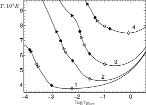
Figure 2: The formation region of Ca I and Ca II lines for solar Ca abundance (filled-in marks) in the accreted gas and for the abundance reduced by 10 times (empty marks). Diamonds correspond to the line of Ca I 5589, rounds correspond to Ca I 4226 line, triangles correspond to the line of Ca II 8498. $T_{ef}=4500$ X, $\log g=4.0$. For various models: 1 – $V_{0}=200$, $\log N_{0}=11.5$; 2 – $V_{0}=400$, $\log N_{0}=11.5$; 3 – $V_{0}=200$, $\log N_{0}=13.0$; 4 – $V_{0}=350$, $\log N_{0}=13.0.$ See text for details.

In the case of the undisturbed atmospheres of CTTS the solar chemical abundances of all elements, including Ca, were assumed. However, due to reasons described in the Introduction we consider the models, where the calcium abundance in the accreted gas, and therefore in the hot spot, can be smaller than solar one. The formation regions of several lines of Ca I and Ca II at various calcium abundances are shown in Fig. 2. It can be seen that for a reduced calcium abundance the line formation regions are shifted to smaller temperatures, and therefore one can expect that the source function at $\tau=1$ as well as the intensity will decrease.

Character of the deviations from the LTE level populations was different for different levels and layers of the hot spot: some levels were overpopulated $(b>1)$ and some were underpopulated $(b<1).$ As an example, we plotted on Fig 3 $b$-factors of levels of some lines, which will be important in the subsequent diagnostics of CTTS’s accretion zone as a function of the optical depth in the center of each line. The upper levels of Ca I lines, shown in the figure, are underpopulated or close to LTE while a lower level is overpopulated, but in the case of Ca II 8498 line departures from LTE are the same for the both levels. We emphasize that the departures from LTE became smaller, when infall gas density or its velocity increase.

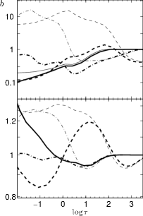
Figure 3: The $b$-factors of Ca I 4226.7 (dashed), Ca I 6162.2 (dash-dotted) and Ca II 8498.0 (solid) lines as function of its optical depth at the line center. Thick curves correspond to upper levels and thin curves correspond to lower levels. In the case of Ca II 8498.0 line, the thick and thin curves are almost merged. The model of the hot spot was calculated for stellar parameters: $T_{ef}=4500$ K, $\log g=4.0$ and for parameters of the accretion flow $V_{0},$ $\log\,N_{0}$: 200, 11.5 (upper panel); 400, 12.5 (lower panel)

It can be seen more clear on Fig. 4, where we plotted $b$-factors of upper and low levels of Ca I 5589 line at the point of the hot spot where line’s central optical depth is equal to 1 as a function of accretion parameters $V_{0}$, $N_{0}.$ The similar behavior is typical for all considered lines of Ca I and Ca II.

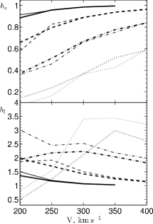
Figure 4: The $b$-factors of the upper (top panel) and the lower (bottom panel) levels of Ca I 5589 at the depth, where the optical depth at the line’s center is equals to 1, as a function of the pre-shock gas velocity $V_{0}$ (in km s^-1). The solid, dashed, dash-dotted, and dotted lines are for $\log N_{0}=13.0,$ $12.5,$ $12.0,$ and $11.5,$ respectively. The thin and thick curves correspond to the models with the stellar temperature $T_{ef}=4000$ K and 5000 K respectively.

3 The calculation of spectrum of Ca and other photospheric lines

To compute the intensity spectrum of a photosphere, we modified the SYNTHE code (Kurucz, 1993; Sbordone et al., 2004). The initial code calculates a LTE spectrum and therefore the source function is assumed to be the same for all lines and equals to the Planck function: $S_{\nu}=B_{\nu}(T)$. To take into account lines with departures from the LTE, we replaced this expression by the general one:

$$S_{\nu}=\frac{j_{\nu}}{\kappa_{\nu}}.$$

In the initial code the factor, which corrects the opacity due to stimulated emission, does not depend on the specific source of the absorption, however in non-LTE case the factor may be different for each $i$-th source of opacity. Therefore an initial expression for the total opacity:

$$\kappa_{\nu}=(1-e^{-\frac{h\nu}{kT}})\sum{\kappa^{0}_{i}(\nu)}$$

should be replaced by:

$$\kappa_{\nu}=\sum\limits_{i}\kappa_{i}(\nu)=\sum\limits_{i}\kappa^{0}_{i}(\nu)\,\left[b_{l}^{i}-{b_{u}^{i}}e^{-\frac{h\nu}{kT}}\right],$$

where $\kappa^{0}_{i}(\nu)$ is an opacity, concerned with an $i$-th source and being calculated in the initial code, and $b_{u}^{i}$, $b_{l}^{i}$ are Menzel’s $b$-factors of upper and low levels for the $i$-th source.

The expression for the total emission coefficient can be written as:

$$j_{\nu}=\frac{2h\nu^{3}}{c^{2}}\,\sum\limits_{i}\kappa_{i}(\nu)\left[\frac{b_{l}^{i}}{b_{u}^{i}}e^{\frac{h\nu}{kT}}-1\right]^{-1}.$$

To calculate a line in LTE approximation, its $b$-factors should be equated to 1.

For some lines of Ca I and Ca II we replaced original values of $\log\,(gf)$ and van der Waals damping parameters by more accurate values – see 1, 4 and 8 columns of Tabl. 4 of Mashonkina et al. (2007) paper. The spectra of the hot spot and the photosphere were simulated with a spectral resolution $R=600\,000$ and for a microturbulence velocity $V_{mic}=2$ km s^-1. To align the spectral resolution with the observed one, the theoretical spectra were broadened by a convolution with a gaussian, a halfwidth of which was adjusted for each order of the echelle spectrum.

To test our code we compared intensity spectra, simulated by the initial program and by our code, in which we set $b_{i}=1$ for all lines. The results completely coincided. We have also compared our calculations of three Ca I lines profiles for the model of the solar atmosphere with the profiles, simulated by L. I. Mashonkina via the SIU program (Mashonkina et al., 2007). The difference of about $\sim 2\%$ in line’s depth was found in the case of Ca I 6439 AA line, for which the difference between LTE and non-LTE profiles was 20%. The depths for the rest considered lines differ even less. Aforesaid allows us to conclude that the modified SYNTHE code works properly.

The additional argument confirming that the program of calculating hot spot spectra works properly looks as follows. Typical energy of photons in optical band is $\sim 2$ eV, and the temperature in the formation region of Ca lines is $\sim 0.7$ eV (see Fig.,2), what means that $\exp(h\nu/kT)\gg 1.$ Then:

$$I_{nLTE}\sim S_{nLTE}(\tau_{nLTE}=1)\sim{\left({b_{u}\over b_{l}}\right)}_{nLTE}\,B_{\nu}\left[T(\tau_{LTE}=1)\right]\sim{\left({b_{u}\over b_{l}}\right)}_{nLTE}\,I_{LTE}.$$

We calculated $I_{nLTE}/I_{LTE}$ values for several lines of Ca I and Ca II from this equation using $b$-factors calculated by our DETAIL code. It appeared that these quantities differed from the same values, derived from our version of the SYNTHE code, less than 20%.

Let discuss now how departure from LTE affects on the intensity spectrum of Ca lines, which are formed in the hot spot, considering it as a plane-parallel slab. If to fix parameters of undisterbed atmosphere then spot’s radiation intensity depends only on the parameters of the accretion shock $V_{0},$ $N_{0}$ and cosine $\mu$ of angle between the line of sight and the normal to the slab.

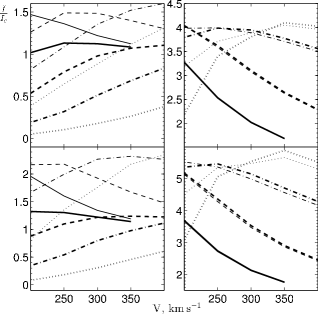
Figure 5: The intensity of Ca I 5589 (left column) and Ca II 8498 (right column) lines at the central wavelength, normalized to the continuum intensity, as a function of a pre-shock velocity of the gas $V_{0}$ km s^-1 for various values of $\log N_{0}:$ the solid, dashed, dash-dotted, and dotted curves are for $\log N_{0}=13.0,$ $12.5,$ $12.0,$ and $11.5$ respectively. The upper and lower rows correspond to $\mu=1$ and $\mu=0.5.$ The thicker and thinner lines correspond to non-LTE and LTE calculations respectively. The parameters of the undisturbed atmosphere are: $T_{ef}=4500$ X, $\log g=4.0.$ See text for details.

To characterize a behavior of a line, we choose a parameter $\xi,$ which is defined as a ratio of the line intensity at the central wavelength to a continuum intensity at $\lambda=\lambda_{0}:$ if $\xi<1$, then the line is an absorption one, and if $\xi>1$, then it is an emission line. $\xi$ values for Ca I 5589 and Ca II 8498 lines are plotted on Fig. 5 as a function of the accretion parameters $V_{0},$ $N_{0}$ and the cosine $\mu.$ For instance, it follows from the figure that the line Ca I 5589 can appear in an absorption as well as in an emission, while the line Ca II 8498 is always an emission line.

We also plotted on the same figure the parameter $\xi,$ calculated in LTE approximation: it can be seen that the differences between LTE and non-LTE values of $\xi$ decreases, when $N_{0}$ and $V_{0}$ increase. It looks strange at the first glance because, according to (2), with increasing of $N_{0}$ and $V_{0}$ the accretion flux $F_{ac}$ also increases, and therefore, the role of radiative processes, which produce the departures from LTE, should be larger. But at the same time the gas density (and therefore, collisional rates) in the hot spot also increases, because the pressure at spot’s upper boundary is proportional to $N_{0}V_{0}^{2}$ (Dodin and Lamzin, 2012).

We have seen on the example of Ca I 5589 and Ca II 8498 lines that the parameter $\xi$ is a function of $V_{0}$ as well as $N_{0}$, however it turned out that the functions $\xi=\xi(V_{0},N_{0})$ were very similar for all optical Ca lines at considered parameters of the accretion flow. Hence nearly identical changes in the intensities of a pair of Ca lines can be obtained by variation of $N_{0}$ as well as of $V_{0}.$ To a larger extent this is correct for pairs of subordinate lines of Ca I, to a lesser extent – for pairs of Ca I-Ca II or pairs, one of which is Ca I 4227 resonant line. At practice it does not allow to determine separately $N_{0}$ and $V_{0}$ parameters from hot spot’s spectrum if to use Ca lines only.

4 The calculation of He I and He II spectrum

Having computed the level populations of helium, we calculated an emerging spectrum as follows. It was assumed that all background radiation with an intensity $I_{\nu}^{0}$ at the frequency of considered spectral line was formed in the layers below this line’s formation region. Then the solution of radiative transfer equation for a slab with a thickness $H$ in the direction, for which a cosine of an angle to the normal to the slab equals to $\mu>0,$ can be written as:

$$I_{\nu}(\mu)=I_{\nu}^{0}(\mu)e^{-\frac{\tau_{\nu}(H)}{\mu}}+\frac{1}{\mu}\int\limits_{0}^{H}{j_{\nu}(z)e^{-\frac{\tau_{\nu}(z)}{\mu}}{\rm d}z},$$

and the total emission coefficient:

$$j_{\nu}(z)=\frac{h{\nu}N(z)\xi_{He}n_{U}(z)}{4\pi g_{U}}\sum\limits_{i}A_{u}^{i}g_{u}^{i}\Psi\left[z,\nu-\nu_{i}\left\{1-\frac{V(z)}{c}\mu\right\}\right].$$

The following notation were used in these expressions. $\nu_{i}$ is a frequency of $i$-th component of a fine structure, $A_{u}^{i}$, $g_{u}^{i}$ are Einstein A coefficient and statistical weight of an upper sublevel of the $i$th component, and $g_{U}$, $n_{U}$ are statistical weight and relative population of the upper level as a whole. Corresponding atomic data were adopted from the CHIANTI v.5.0 atimic database (Dere et al., 1997; Landi et al, 2006). Note by the way that line’s central wavelength was defined as weighted average over wavelengths of all $i$th components of the fine structure with $(gf)_{i}$ weights. $N(z)$ and $V(z)$ are a number density and a velocity of the gas, which were adopted from models of post-shock cooling zone (Lamzin, 1998) and hot spot (Dodin and Lamzin, 2012). The velocity of the gas settling $V(z)$ was equated to zero in the hot spot. Helium abundance $\xi_{He}=0.1.$

$\Psi(z,\nu)$ is line’s absorption and emission profile normalized as $\int\Psi(z,\nu){\rm d}\nu=1.$ For He I lines we took into account Stark broadening according to Dimitrijevic & Sahal-Brechot (1984). In the case of He II lines we used Doppler profile at $T>3\times 10^{5}$ K and at lower temperatures (it corresponds to higher densities in our models) we took in to account Stark broadening by an interpolation of Schöning and Butler (1989) tables. The tables cover the whole necessary density range, but there is no data for $T<10^{4}$ K. In this case we formally used the same profile as for $T=10^{4}$ K, but it cannot lead to significant error, because He II is practically absent at $T<10^{4}$ K – see Fig. 1.

The absorption coefficient was calculated as follows:

$$\kappa_{\nu}(z)=\frac{\pi e^{2}}{m_{e}c}N(z)\xi_{He}\left[\frac{n_{l}(z)}{g_{L}}-\frac{n_{u}(z)}{g_{U}}\right]\sum\limits_{i}(gf)_{i}\Psi\left[z,\nu-\nu_{i}\left\{1-\frac{V(z)}{c}\mu\right\}\right].$$

where $n_{l}$, $n_{u}$, $g_{L}$, $g_{U}$ are the populations and statistical weights of lower and upper levels, which are not splitted into components of the fine structure. The optical depth of a line in this case differ a little from the same quantity, derived in the program of the level population, because we did not consider there line’s fine structure and assumed that the line has Voigt profile.

The method of a calculation of $I_{\nu}^{0}$ was described in the previous section. The calculations of $I_{\nu}$ were carried out for the same set of $\mu$-values and on the same frequency grid as for $I_{\nu}^{0}.$

We found from the comparison of He I and He II lines fluxes, calculated with our code and with the Cloudy08 code, that all differences in the results were completely caused by differences in the level populations due to differences in used atomic data (see above). This allows us to conclude that our code works properly.

We will use in what follows the model of a round homogeneous accretion spot, i.e. will assume that the accretion flow has the shape of a circular cylinder, across which $N_{0}$ and $V_{0}$ parameters are the same everywhere. At first we separately calculated spectra of the hot spot and undisturbed atmosphere. Then we choosed relative area $f$ of the spot and its position at stellar disk, defined by the angle $\alpha$ between spot’s axis of simmetry and the line of sight, and calculated resulting spectrum of the ”star $+$ spot” system by integration of specific intensity over visible stellar hemisphere – see Dodin & Lamzin (2012) for details.

We will illustrate the results of our simulation of helium spectrum on the example of He II 4686 line. Note by the way that CTTS are late-type stars so helium lines are absent in their photospheric spectra. Consider a set of spectra of non-rotating star with $T_{ef}=4000$ K, $\log g=4.0,$ which has an accretion spot on its surface. Free parameters of the problem are filling factor $(f=0.01,$ 0.03, 0.06, 0.1, 0.15, 0.2), spot’s position $(\alpha=0^{o},$ $60^{o})$ and parameters of the accretion flow: $\log N_{0}$ from 11.5 to 13.0 with a step of 0.5, $V_{0}$ from 200 to 400 km s^-1 with a step of 50 km s${}^{-1}.$

He II 4686 line will be characterized by an equivalent width of a part of its profile $\Delta v$ from -30 to 30 km s^-1, taking into account all photospheric lines inside this velocity range. The accretion power will be characterized by the veiling $r_{c}$ of a photospheric spectrum due to a continuum emission only rather than total veiling $r$, because it varies from line to line. Let us remind that $r_{c}$ is defined as the ratio of the flux from accreting star $F_{\lambda}(\lambda)$ to that of non-accreting star $F_{\lambda}^{0}(\lambda)$:

$$r_{c}(\lambda)=\frac{F_{\lambda}}{F^{0}_{\lambda}}.$$

The relation between $r_{c}$ and total veiling $r,$ defined by Eq.1, depends on the accretion flow parameters: at small values of $F_{ac}$ the veiling is caused by lines, and $r$ is several times greater than $r_{c}$ (Dodin and Lamzin, 2012).

It appeared that at a fixed angle $\alpha$ the relation between $r_{c}$ and He II 4686 line equivalent width is sensitive to infall gas density $N_{0}.$ It can be seen from Fig. 6 that models with the same value of $N_{0},$ but with various other parameters $V_{0},$ $f$, form bands, which are well separated at the chosen $\lg N_{0}$ step of 0.5, especially at a high veiling.

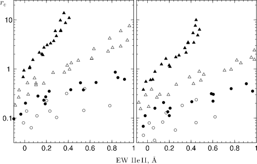
Figure 6: The veiling $r_{c}$, caused by a continuum emission, in the vicinity of He II 4686 line as a function of its equivalent width. The models were simulated for the values of $V_{0}$ from 200 to 400 km s^-1 with a step of 50 km s^-1 and $f=0.01,$ 0.03, 0.06, 0.1, 0.15, 0.2 at values of $\log N_{0}=11.5$ (empty rounds), $12.0$ (filled-in rounds), $12.5$ (empty triangles), $13.0$ (filled triangles). The left and right panels of the figure for the cases where the line of sight makes, respectively, the angles $\alpha=0^{o}$ and $\alpha=60^{o}$ with the axis of the spot. Parameters of a star are $T_{ef}=4000$ K, $\log g=4.0$.

The veiling $r_{c}$ is a purely theoretical parameter, because only the upper limit of $r_{c}$ can be found from observed spectrum as a minimal $r$ of all photospheric lines in the spectral region of interest. Therefore, the Fig. 6 is no more than an illustration of a sensitivity of some spectral details to parameters of the accretion flow, in our case, to gas density $N_{0}.$

5 A comparison of the simulated spectra with observations

High resolution spectra of CTTS, which we compared with calculations, were adopted from the Keck Observatory Archive http://www2.keck.hawaii.edu/koa/public/koa.php and (in the case of TW Hya) from the VLT archive http://archive.eso.org/eso/eso_archive_main.html. We used automatically extracted and calibrated spectra, because did not found any artifacts, which can influence to our conclusions. Each observed spectrum was transformed into the stellar rest frame by shifting it as a whole (by radial velocity) until a coincidence of photospheric lines positions with that of theoretical spectra. In order to compare the observed and simulated spectra of CTTS, we normalized both to continuum level. It appeared difficult to derive continuum level at wavelengths shortward 4000 Å for all stars except TW Hya. Due to this reason we compare spectra of the stars with our simulations only at wavelengths $\lambda>4000$ Å, what, in the particular, did not allow us to use Ca II H and K lines for a diagnostic.

Even in the model of a homogeneous circular spot there are quite a lot parameters that characterize a star ($T_{ef}$, $\log g$, $V_{mic},$ an equatorial rotational velocity $V_{eq}$, an inclination $i),$ an accretion shock $(V_{0},$ $N_{0}$) and a spot ($f,$ $\alpha).$ At first we would like to describe, how we determined these parameters for each spectrum of CTTS.

The stellar parameters were adopted from the literature, except a few cases, when we derived them by ourself to reach better agreement with observations. Reliable determinations of the microturbulence velocity for CTTS are apparently absent and we always assumed $V_{mic}=2$ km s^-1. The parameters of 9 stars, spectra of which have been compared with calculations are collected together in the Table 1.

Table 1: Stellar parameters.

Star	$T_{ef},$ K	$\log g$	$i,^{o}$	$V_{eq},$ km s-1
GM Aur	$4500^{b}$	$4.0^{k}$	$50^{j}$	$17^{h}$
BP Tau	$4000^{a}$	$3.5^{a}$	$50^{a}$	$15^{a}$
DK Tau	$4250^{b}$	$4.0^{b}$	$50^{g}$	$15^{h}$
DN Tau	$4250^{b}$	$4.0^{b}$	$30^{e}$	$17^{f}$
GI Tau	$4250^{i}$	$4.0^{g}$	$70^{g}$	$9^{g}$
GK Tau	$4250^{k}$	$3.5^{g}$	$50^{g}$	$20^{g}$
V836 Tau	$4500^{k}$	$4.0^{k}$	$60^{k}$	$16^{k}$
DI Cep	$5500^{k}$	$3.5^{c}$	$60^{c}$	$25^{c}$
TW Hya	$4000^{d}$	$4.0^{d}$	$10^{d}$	$16^{d}$
References: a – Donati et al. (2008); b – Schiavon et al. (1995); c – Gameiro et al. (2006); d – Donati et al. (2011); e – Bouvier and Bertout (1989); f – Smith (1994); g – Johns-Krull and Valenti (2001); h – Hartmann and Staufer (1989); i – Kenyon and Hartmann (1995); j – Gräfe et al. (2011); k – $T_{ef},$ $\log g,$ $V_{eq}$ were chosen by us, and $i$ adopted arbitrary.

The parameters of an accretion shock and a hot spot were found as follows. Pre-shock gas number density $N_{0}$ was determined from the comparison of veiling $r_{c}$ in the vicinity of He II 4686 line and $EW$ of this line (see the previous section and Fig. 6). One can assert that an error of $N_{0}$ is significantly less than the density step of our shock models grid, which is equal to 0.5 dex, because it appeared impossible to reproduce simultaneously observed veiling and $EW$ of He II 4686 line for such deviations from derived value of $N_{0}$ by variation of other parameters.

We discovered that He II 4686 line consist of two components: one is strong and narrow, and second is broad and weak. To our knowledge, the broad component of He II 4686 line has never been described before, possibly because it is masked by a blend of photospheric lines. But if to subtract calculated veiled photospheric spectrum from the observed one, then it turns out that the profile of He II 4686 line is practically coincide with that of He I 5876 line (see Fig. 7), for which an existence of the broad component is well recognized. We used only a central peak and a blue wing of He II 4686 line to derive $N_{0}.$

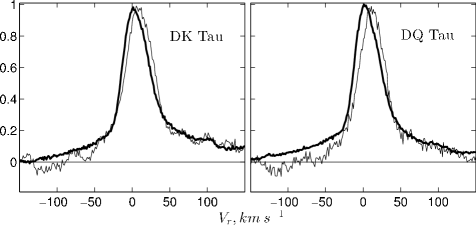
Figure 7: Profiles of He I 5876 (thick curve) and He II 4686 (thin curve) lines normalized to their maximum in spectra of DK Tau (JD 2 454 487.872) and DQ Tau (JD 2 455 144.123) after the substraction of the veiled photospheric spectrum.

Thus, it can be concluded that broad components of both He lines in considered stars are formed in the same region. As far as broad components of the lines are redshifted, it is naturally to assume that they are formed somewhere in pre-shock accretion flow, which links the disc and the star.

Having derived $N_{0},$ it is possible to determine $V_{0}$ by analizing SED of the veiling continuum, which can be characterized by $r_{c}=r_{c}(\lambda).$ It is caused by the fact that hot spot effective temperature and $r_{c}(\lambda)$ depend on $V_{0}$ only if $N_{0}$ is fixed. Aforesaid is illustrated by Fig. 8, on which $V_{0}$ is plotted as a function of a ratio of the veilings $r_{c}$ in the vicinity of He II 4686 line and in the region 6000-6500 ÅÅ for the model of a star with $T_{ef}=4000$ K, $\log g=4.0$ and the same parameters of the accretion spot, as on Fig. 6. It is seen that for the chosen spectral band $V_{0}$ can be derived more precisely in the case of high density and the result weakly depends on $\alpha$ and $f.$ The figure is presented as an illustration of the method only: in reality we fitted not only $r_{c}(\lambda)$ but also total veiling $r=r(\lambda)$ in the whole observed spectrum.

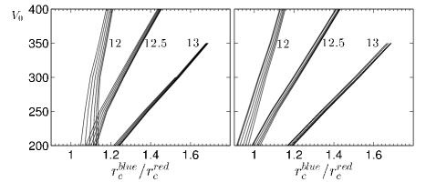
Figure 8: Dependence of pre-shock velocity $V_{0}$ (in km s^-1) on the ratio of veilings $r_{c}$ in the blue (near the He II 4686 line) and red (6000-6500 ÅÅ) spectral bands. Different groups of lines correspond to various values of $\log N_{0}$ (written near the group), and various lines within each group correspond to various filling factors. Models at the left panel corresponds to spot’s orientation $\alpha=0^{o}$ and at the right panel – to $\alpha=60^{o}.$ The parameters of the star are: $T_{ef}=4000$ K, $\log g=4.0.$

Note that while hot spot models were calculated at a discrete grid of the parameters $V_{0}$ (200-400 km s^-1 with a step of $50$ km s${}^{-1})$ and $\log N_{0}$ (11.5-13 with a step of 0.5 dex), we calculated spectra also for intermediate values of $V_{0},$ $N_{0},$ obtained by means of 2-D linear interpolation of specific intensity $I_{\nu}(\mu,\lambda).$

Having derived accretion shock parameters $N_{0}$ and $V_{0},$ one can find parameters of the spot. An observed quantity, suitable for this purpose, is veiling by lines or, in other words, an intensity of the narrow component of metal’s emission lines, which fill in to various extent respective photospheric lines. Different brightening low $I_{\nu}(\mu)$ of lines and continuum allows to determine the angle $\alpha$ and filling factor $f$ from the relations between equivalent widths of narrow components of emission lines and $r_{c}$ value. Fig. 9 illustrates this statement on an example of two lines: Ca I 4226.73 resonant line, which always has an emission core in CTTS spectra and Fe II at 4233.17 Å line located near the first.

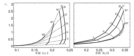
Figure 9: $r_{c}$ value in the vicinity of Ca I 4226.73 (left panel) and Fe II 4233.17 (the right panel) lines as function of EW (in Å) of these lines (see text for details). Thin curves correspond to models with the same relative area $f,$ values of which (in %) are indicated at the figure. Dots at these curves mark models with $\alpha$ that differs in $10^{o}.$ Bold curves connect models with different $f$ but equal $\alpha$. Additional parameters of the models are: $T_{ef}=4000$ K, $\log g=4.0,$ $\log N_{0}=13.0,$ $V_{0}=200$ km s^-1.

The narrow emission components of both lines are located inside the broad (photospheric) Ca I 4226.73 line, therefore it is better to measure their equivalent widths relative to the flux at the nearby point of the photospheric line wing, rather than relative to uncertain continuum level. These points were chosen in theoretical spectra at $\lambda=4226.63$ Å and $\lambda=4233.30$ Å for Ca I 4226.73 and Fe II 4233.17 lines respectively.

When suitable values of $\alpha$ and $f$ were choosen to reproduce observed profile and intensity of Ca I 4226.73 line the model with solar calcium abundance in accreted gas $\xi_{Ca}$ also reproduced these quantities for all other Ca I lines as well as for Fe II 4233.17 line. The only exception was TW Hya for which we tried to use models with $\xi_{Ca}$ 3 and 10 times less than solar value.

The using of $\xi_{Ca}$ as a free parameter and LTE-spectra of Fe II in our approach makes determination of $f$ and $\alpha$ values somewhat uncertain, however there is no sense to determine these parameters with high accuracy in the frame of simple round homogeneous spot model. Due to the same reason we choose the best fit model by means of visual comparison of simulated spectra with observed, i.e. did not use any mathematical optimization technique.

However it should be noted that the model allows in principle to determine not only the angle $\alpha,$ but a latitude $\theta$ and a longitude $\varphi$ of spot’s center on the stellar surface, using the relation:

$$\cos\alpha=\cos\theta\cos i+\sin\theta\sin i\cos\varphi,$$

where $i$ is an inclination of the rotational axis of the star to the line of sight. We measured the angle $\theta$ from the nearest pole, and the angle $\varphi$ from the central meridian in the direction of stellar rotation.

Spot’s position at stellar surface relative to the Earth charcterized by $\alpha$-angle varies periodically due to variations of $\varphi,$ while $i$ and $\theta$ angles do not vary. It means formally that parameters $i,$ $\theta$ and $\varphi$ can be found by an analysis a few $(\geqslant 3)$ spectra, obtained at different rotational phases.

In addition in spectra of rotating star the position of an emission component inside respective absorption line varies with time due to Doppler effect. Therefore, observed line profiles should looks different at different $\varphi$. The described effect is manifested in the form of periodical variations of radial velocities of CTTS photospheric lines (Zaitseva et al., 1990; Petrov et al.,2001). Fig. 10 shows that the shape of absorption lines in high-quality spectra can be sensitive enough to the angle $\varphi.$ If an asymmetry of photospheric lines profiles was noticeable in the observed spectrum, we determined $\theta$ and $\varphi,$ instead of $\alpha$ (for illustrative purposes only) adopting $i$ from the literature – see table 1.

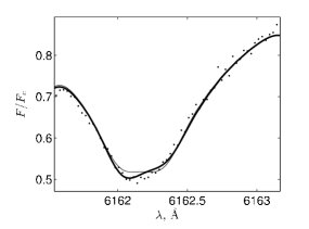
Figure 10: Comparison of Ca I 6162.17 line profile in DK Tau spectrum at JD 2 454 487.866 (dots) with simulated profiles: the thick and thin curves correspond to models with $\varphi=15^{o}$ and $\varphi=0^{o}$ respectively. Other parameters of the models can be found in Tabl. 1 and Tabl. 2

But in some analyzed spectra profiles of photospheric lines had a symmetrical shape, while the veiling by lines was noticeable, judging from the theoretical spectrum. Apparently it means that accretion zone (spot) of these stars is extended in longitude in agreement with numerical simulations (Romanova et al. 2004). We posed $\varphi=0$ in such cases and determined $\theta$ only.

Table 2: Acretion spot parameters

The star	JD 245…	$V_{0}$	$\log N_{0}$	$f$, %	$\theta$,o	$\varphi$,o	$L_{ac}/L_{*},$ %	$\dot{M}_{ac}$
GM Aur	3337.850	280	13.0	1.5	0	0	15	8.8
	3984.035	290	13.0	1.6	0	0	18	9.7
	4717.048	300	13.0	1.4	0	0	18	8.8
BP Tau	1883.003	300	13.0	2.0	30	0	40	13
	2535.982	350	13.0	2.0	20	0	64	15
	3301.985	325	12.9	1.3	0	0	27	7.2
	3368.772	350	13.0	0.8	30	0	26	5.9
	3984.022	300	12.6	3.0	20	0	24	7.5
	4487.837	350	13.0	1.3	20	0	42	9.6
	4544.739	335	13.0	2.0	20	0	56	14
	4717.052	350	13.0	1.2	20	0	39	8.8
	4807.915	350	13.0	1.5	20	0	48	11
DK Tau	4487.866	300	11.9	12	40	15	15	6.0
	4487.872	300	11.9	12	40	20	15	6.0
DN Tau	5135.041	230	12.2	3.0	30	60	3.4	2.3
	5284.753	280	13.0	1.2	20	50	16	7.1
GI Tau	4487.930	330	13.0	2.0	40	-40	42	14
GK Tau	4487.924	270	13.0	1.5	10	0	17	8.5
V836 Tau	4806.967	230	12.5	5.0	30	60	9.0	7.6
DI Cep	4609.131	260	13.0	4	40	-10	15	22
TW Hya	4157.875	350	13.0	1.0	10	0	32	7.3
	4158.607	360	12.8	1.0	10	0	22	4.8
Note. – $V_{0}$ in km s-1, $N_{0}$ in cm${}^{-3},$ $\dot{M}_{ac}$ in ${(R_{*}/R_{\odot})}^{2}\times 10^{-9}M_{\odot}/$year. The quality of the spectra of BP Tau allows to reliably determine only the density $N_{0}.$ For TW Hya $\xi_{Ca}/\xi_{Ca}^{\odot}=0.3$ and 1 for all other stars.

Following the described algorithm, we have determined accretion parameters of all CTTS from the Tabl. 1 and presented them in the Tabl. 2. It can be seen from this table that the majority of stars accretes a gas with a number density $N_{0}>3\times 10^{12}$ cm${}^{-3}.$ It turned out that at such high densities LTE and non-LTE spectra were similar and reproduced observed depth of all subordinate lines of Ca I in optical band and the narrow emission component of Ca I 4226.73 resonant line. An example is the star GM Aur $(\log N_{0}=13),$ for which parts of the spectrum are shown on Fig. 11. For every star except TW Hya, which will be discussed below, an acceptable agreement between the calculations and the observations was achieved at the solar abundance of calcium. Moreover, depths of photospheric lines of other elements are also reproduced in our models with a good accuracy.

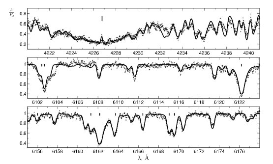
Figure 11: Some regions of the spectrum of GM Aur at JD 2 453 337.850 (crosses), which contain Ca I lines, positions of which are marked by vertical bars. In the case the results of non-LTE (thick line) and LTE (thin line) calculations at the same parameters of the accretion spot practically coincide.

However, in the case of DK Tau, for which $\log N_{0}=11.9,$ the difference between LTE and non-LTE models is very noticeable, see Fig. 12. If the model is chosen so that it reproduces the equivalent width of the He II 4686 line and SED of the veiling continuum, then the narrow emission components of Ca I at solar abundance of calcium are much stronger than the observed ones. The use of non-LTE calculations for calcium allows to achieve a good agreement with observations without assumptions about the depletion of this element. The model are well reproduce a lot of absorption lines of other elements, but for some lines of Fe, for instance Fe I 4235.9 and Fe I 5586.8, the model predicts a more strong emission component than observed. It indicates probably that it is necessary to consider non-LTE effects not only for calcium, but also for iron in the case of DK Tau.

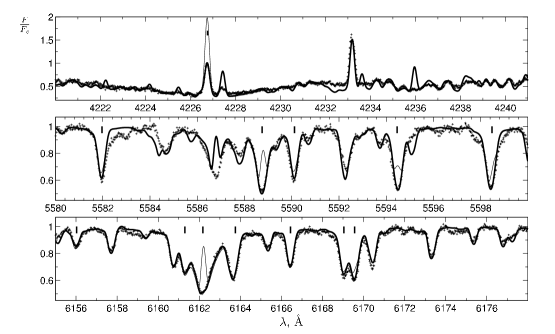
Figure 12: The same as in Fig. 11, but for DK Tau (JD 2 454 487.866). The thick and thin curves correspond to a non-LTE spectrum for calcium lines and a LTE spectrum for all lines at the same parameters respectively.

Fig. 13 shows how the models with the same parameters reproduce observed spectra of GM Aur and DK Tau in the vicinity of He II 4686 line. The figure demonstrates also how gas density $N_{0}$ affects on EW of the line.

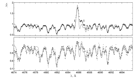
Figure 13: The region of the spectra of DK Tau (top panel) and GM Aur (bottom panel) in a vicinity of He II 4686 line. Julian dates and the parameters of the models, the spectra of which are shown by the thin curve, are the same as in Fig. 11, 12. Positions of Ca I lines are marked by vertical bars.

As we noted in the section, devoted to the calculations of helium level population, a probable deviation of LTE-distribution of $T(\tau)$ from the true structure in the upper layers of a hot spot and uncertanties in the collisional cross sections from upper levels of He I do not allow to trust to the simulated profiles of He I. It turned out that intensities of He I 4471, 4713, 5016, 5876, 6678, 7281 ÅÅ lines predicted by our models were significantly smaller than observed. The ratios of an equivalent widths of these lines are also disagree with observations especially in the case of He I 4471 line ($n=4\rightarrow 2$ transition): its $EW$ in observed spectra is comparable with $EW$ of 5876 Å line $(n=3\rightarrow 2$ transition), while in the simulated spectra 4471 Å line is significantly weaker than 5876 Å line and almost invisible in the spectrum. Aforesaid is illustrated by Fig. 14 on examples of GM Aur and DK Tau.

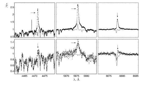
Figure 14: The region of the spectra of DK Tau (upper panel) and GM Aur (lower panel) in the vicinity of He I 4471, 5876 and 6678 lines. Julian dates and parameters of the models, the spectra of which are shown by the thin curve, are the same as for Fig. 11 and 12 respectively. The absorption feature at the left from He I 6678.16 line is photospheric FeI 6677.99 line.

Unfortunately we could not use lines of Ca II for the diagnostic in the case of CTTS, spectra of which were taken from Keck Observatory Archive. In spectra of these stars only Ca II H and K resonance lines and the infrared triplet (IRT) at $\lambda=8498.0,$ 8542.1, 8662.1 ÅÅ have significant intensity. As we have noted before, the difficulties with determination of continuum level at $\lambda<4000$ Å did not allow us to use the H and K lines. What about IR triplet lines they either were out of observed spectral range or consisted almost fully from broad component so that the narrow component cannot be extracted. At the same time it is necessary to note that other Ca II lines, which are absent in the spectra of investigated stars, also have negligible intensity in spectra of our models.

These problems have been overcome in the case of TW Hya, for which spectra were retrieved from the VLT archive. For this star the relative intensity of the He II 4686 line and the SED of the veiling continuum were successfully fitted by a model of the homogeneous spot, but having assumed that the calcium abundance in the falling gas is three times smaller than solar. Note, that the age of TW Hya is about 8 Myr (Donati et al., 2011), i.e. it is significantly older than other considered stars, therefore, the depletion of calcium in the accreted gas due to its accumulation in heavy grains looks resonable.

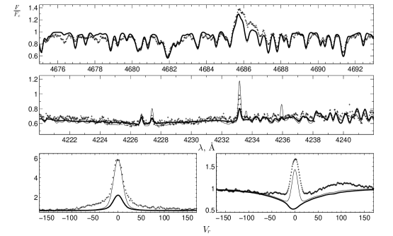
Figure 15: Some regions of TW Hya spectrum (JD 2 454 157.875) in the vicinity of He II 4686 line (upper panel) and Ca I lines (middle panel) as well as observed profiles of Ca II K line $(\lambda=3933.7$, left lower panel) and $\lambda=8662.1$ Å line of Ca II IR triplet (right lower panel). The crosses correspond to the observed specra. The thick curve corresponds to the model of the homogeneous spot with parameters from the Tabl. 2. The thin curve corresponds to the model of the two-component spot, the parameters of which are given in the text.

However, as can be seen from the figure, the intensity of the narrow component of the Ca II lines is significantly smaller than the observed. In order to increase it, we need to decrease pre-shock density $N_{0},$ but then the intensity of He II 4686 line became larger than the observed. This contradiction can be overcomed by assuming an inhomogeneity of the spot, namely, by assuming that the spot with high densities and velocities of the falling gas is surrounded by an accretion zone with lower values of $N_{0}$ and $V_{0}.$

To illustrate it, we have calculated two-component spot’s model for TW Hya. The model assumes that the central region with $V_{0}=370$ km s^-1, $\log N=13.0,$ $f=0.008,$ $\varphi=0^{o},$ $\theta=10^{o}$ is surrounded by a coaxial ring zone with $V_{0}=250$ km s^-1, $\log N_{0}=11.5$ and $f=0.06.$ As in the case of the homogeneous spot, the abundance of calcium was adopted 3 times smaller than solar. The simulated spectrum of two-component spot are shown on Fig. 15 by a thin curve. We did not try to choose the parameters of the composite spot in order to achieve the best agreement with observations. The figure demonstrates only that inhomogenious spot model allows to reproduce the observed flux of the Ca II lines, not disturbing the agreement between the calculations and the observations for veiling and other lines.

The ratio of accretion to stellar luminosities and mass accretion rate, presented in two last columns of the Tabl. 2, were calculated from the relations:

$${L_{ac}\over L_{*}}={fF_{ac}\over\sigma T_{ef}^{4}},$$

$$\dot{M}_{ac}=4\pi R_{*}^{2}f\mu m_{p}N_{0}V_{0},$$

where $\mu\simeq 1.3$ is the average molecular weight, $m_{p}$ is the proton mass.

$\dot{M}_{ac}$ value in the table was calculated for stellar radius $R_{*}=R_{\odot},$ because we did not determine here $R_{*}$ and the values from the literature is very unreliable. Note that if there are two accretion spots with similar parameters, which are located in diametrically opposite regions on the surface of CTTS, then the values of $L_{ac}/L_{*}$ and $\dot{M}_{ac}$ from the table should be increased by 2 times.

Calvet and Gullbring (1998) investigated the first six stars from our Tabl. 2 in the frame of their model, which assumes that the spot emits in continuum only. $F_{ac}$-values for these stars, obtained by Calvet and Gullbring are, in average, twice larger than our, while filling factors $f,$ vice versa, are a few times smaller. Note that, in contrast to our paper, Calvet and Gullbring used $V_{0}$-values derived from the assumption that they are free fall velocity at 5$R_{*}$ and adopting masses and radii of stars found by Gullbring et al. (1998) from evolutionary tracks. These $V_{0}$-values are systematically smaller than our.

For five considered CTTS out of nine we have analyzed more than one spectrum – see Tabl. 2. In the case of DK Tau and TW Hya the spectra were taken with an interval less than one day, and the parameters of the spot, derived from them, differ just a little. A good repeatability of the parameters can be noted also for GM Aur. The signal-to-noise ratio of BP Tau spectra is relatively low, and due to this reason we can reliably determine $N_{0}$ value only, which in one case out of nine differs significantly from other. Only for DN Tau the temporal variations of the parameters were significant. It can be assumed that in this case the properties of the accretion stream were changed indeed, because these two spectra are visually differs from each other.

Conclusion

It is generally recognised that emission spectrum of CTTS is a consequence of a magnetospheric accretion of matter from a protoplanetary disk, but the spectrum has not been reproduced quantitatively until now. It raises doubts about the reliability of the existing estimates of the parameters of the accretion flow in CTTS, general characteristics of young stars and the interstellar and/or circumstellar extinction $A_{V}$ for these objects. A simulation of CTTS spectrum is complicated by the fact that most of emission lines consist of a narrow and a broad components, which are formed in regions with very different physical conditions, geometry and velocity field.

The difference is so great that at a present day narrow and broad components of the emission lines are being modelled independently of each other. It introduces an uncertainty in a process of a comparison of simulated intensity and profiles of one component due to the a priori unknown contribution of the second. This problem is especially serious in the case of the broad components, because they are formed in a moving gas of the magnetosphere of CTTS, therefore, separation of the components, which is used now, by means of a decomposition of the observed profile into a pair of gaussians cannot be considered as a serious basis for a comparison of simulations with observations. In addition, the simulation of profiles of the broad component is a very laborious and multiparameter problem, which requires a simultaneous solution of 3-D radiation transfer and MHD equations (Kurosawa and Romanova, 2012).

We have seen on an example of He II 4686 and Ca II lines that the broad component complicates comparison of the simulated spectrum of the hot spot with observations. At the same time, our calculations reproduce well profiles of the most lines of neutral metals, for instance Ca I. It means that the broad component is almost absent in these lines. If we reconstruct the spectrum of the hot spot by using such lines, then the profiles of the broad component can be found by substracting the simulated profiles from observed ones. In this paper such approach has allowed us for the first time to discover the broad component in He II 4686 line.

Nevertheless, the main purpose of our modeling is to determine a shape of the accretion spot and distributions of the parameters $V_{0}$ and $N_{0}$ within it. Moreover, the stellar parameters should be determined, namely: $T_{ef},$ $R_{*},$ $i,$ $V_{eq}$ and $A_{V}.$ This problem can be solved by Doppler imageing, using the dependence of $I_{\nu}=I_{\nu}(\mu),$ calculated for as wide as possible spectral range for a comprehensive grid of the parameters. Calculations, performed by Dodin and Lamzin (2012), and in this work are the first steps in solution of this problem.

A good agreement with observations allows to trust to the conclusion that the most of considered stars accretes matter with pre-shock gas density $>3\times 10^{12}$ cm${}^{-3},$ although this conclusion we obtained in the framework of the homogeneous circular spot model. Our $N_{0}$ value found for TW Hya coincides with an estimation of Kastner et al. (2002) derived from X-ray observations, but in the case of BP Tau Schmitt et al. (2005) found $N_{0}$ an order of magnitude smaller than our value.

It turns out that at such density the spectrum of Ca I as well as of other metals are close to LTE. Taking into account a simplicity of our model, it is difficult to say about a reliability of our conclusion about a depletion of calcium in the falling gas in case of TW Hya. However, TW Hya is older than other considered stars in a few times, therefore the depletion of calcium in the falling gas due to its accumulation in heavy grains is possible exactly for this star.

For further progress in the mapping of CTTS’s accretion spots the following should be done.

1) The appropriate observational data should be prepared. At the beginning all available spectra of CTTS should be carefully processed: recall that we used spectra after automatic processing in this study. The simulated spectra have been compared with spectra, which were normalized to continuum level for each echelle order, therefore the obtained results do not depend on the interstellar reddening. A good agreement of observed spectra with simulated ones, for which $F_{\lambda}=F_{\lambda}(\lambda)$ dependence is known, means that we know stellar spectrum, undistorted by interstellar reddening. Hence if we obtain from observations $F_{\lambda}(\lambda)$ dependence, then we could find not only $A_{V},$ but also try to derive the dependence $A_{\lambda}(\lambda).$ If the dependence $F_{\lambda}(\lambda)$ is obtained in absolute units, then we could also find luminosity and radius of a star.

2) Non-LTE structure of upper layers of the hot spot should be calculated. It will allow to calculate more accurately an emission spectrum of He I as well as of hydrogen. By the way, we calculated the non-LTE spectrum of hydrogen, but not used in the diagnostics due to two reasons: at first, profiles of Balmer lines are dominated by the broad component and secondly, the hydrogen lines are formed exactly in the upper layers of the hot spot.

Before this work we have belived that narrow component of H and He, in contrast to Ca, are formed equally in the hot spot and in a moving gas in the postshock cooling zone. For an uniform calculation of the level populations in regions with very different physical conditions we used the escape probability approach. However, it is clear now that the main flux of these lines are formed in the hot spot, therefore in the future the calculation of the level populations of He and H should be carried out just like for Ca.

3) To identify as many as possible lines in CTTS spectra, which are sensitive to variation of accretion flux and stellar parameters: non-LTE calculations should be carried out, at least, for Fe, Mg, Ti and Na. These lines will be used in the future for Doppler mapping of CTTS. For example it has been shown in this work that Ca I at 4226.7Å resonance line is sensitive to spot’s orientation relative an observer, while, at fixed veiling, the line of He II at 4686Å and the lines of Ca II are sensitive to pre-shock gas density.

4) X-ray and UV spectra of the accretion shock should be calculated for the parameters $\log N_{0}>13$ and $V_{0}>400$ km s${}^{-1},$ i.e. larger than used by Lamzin (1998), because there are reasons to suppose that they may be necessary to model spectr of some CTTS.

5) Lines of some important molecules, which have not been included yet in our simulation of spectra, should be added, for instance, TiO, because the molecular lines are typical for late type stars. What is more in addition to the hot spot, cold spots may also present on the surface of CTTS (Donati et al., 2011).

We wish to thank L.I. Mashonkina for useful discussions, for assistance in testing the programs and for the atomic data for calcium; referees for usefull notes and P.P.Petrov, who drew our attention to the problems with interpretation of veiling of Ca I lines in spectra of CTTS. The paper based on observations made with ESO Telescopes at the La Silla Paranal Observatory under programme ID 078.A-9059. This research has made use of the Keck Observatory Archive (KOA), which is operated by the W.M. Keck Observatory and the NASA Exoplanet Science Institute (NExScI), under contract with the National Aeronautics and Space Administration. Principal investigators of the observations were P. Butler, G. Marcy, S. Vogt, G. Herczeg, J. Johnson, A. Sargent, L. Hillenbrand. The work was supported by the Program for Support of Leading Scientific Schools (NSh-5440.2012.2).

The Appendix. The model of the helium atom

The model of the helium atom, used in our calculations, includes energy levels of He I up to the principal quantum number $n=7$ with an orbital splitting and components of the fine structure, energy levels of He II up to $n=10$ without the orbital splitting and the state of He III. Thus, 66 energy levels were included in our model, however at the calculation of the level population, the levels of He I with $n=4-7$ and He II with $n=6-10$ were combined into the superlevels. A relatively small number of the levels in the model is primarily caused by the lack of precise values of rate coefficients for collisional excitation and ionization from upper levels. In other words, it is reasonable to assume that the increase in accuracy due to a larger number of levels will be compensated by low quality of the atomic data for these levels.

Sublevels of He I and He II superlevels assumed to be populated according to the Boltzmann distribution. Due to this reason it was not necessary to consider electron transitions within the superlevel. Transitions between the superlevel $S$ and other levels $n$ of the atom are taken into account by effective transition rates $C,$ which were obtained by averaging of transition rates $C_{Sp\rightarrow n}$ from a sublevel $Sp$ to level $n$ over the Boltzmann distribution for the sublevels $Sp$. Transition rates from the levels $n$ to the sublevels $Sp$ of the superlevel $S$ are calculated by a simple summation. This approach is fully justified at the high density in an accretion column: test calculation without the combination of the levels leads to the same results and shows that the upper levels are indeed populated according to the Boltzmann distribution.

To get a sense of the influence of the number of levels, taken into account in He I and He II, on the accuracy of the results, we used the Cloudy08 code (Ferland et al., 1998). As was noted in Sect.1 the Cloudy08 code and our calculations give similar results for a model of a homogeneous slab with parameters similar to the parameters of the gas in the formation region of He I and He II lines: $T=30\,000$ K, $N=10^{14.5}$ cm${}^{-3},$ slab thickness $H=10^{3}$ cm, blackbody radiation field with $T=30\,000$ K and a dilution factor $10^{-3}.$

At first we have calculated, using the model of the slab, the optical depth of a few lines of He I and He II in the case of the atomic model, which included 7 levels for He I and 10 for He II. Then we have repeated the calculation, but taking 17 levels for He I and 20 for He II. It appeared that relative difference in optical depths of various lines of He II with low level principal quantum number $n=1-4$ was about 0.5%. In the case of He I the difference for $n=1-2$ is less than 1%, and for $n=3$ it is about a few percents. Analogous tests for the models with $N=10^{13}$ and $N=10^{15}$ cm^-3 have led to similar results and we concluded that the number of the levels in our atomic model was sufficient to solve the considered problem.

References

- [1] Batalha C. C., Stout-Batalha N. M., Basri G., Nerra M. A. O., Astrophys. J. Suppl. Ser. 103, 211 (1996).
- [2] [0.15cm]
- [3] Berestetskij V. B., Lifschitz E. M., Pitajevskij L. P., Quantum Electrodynamics . Nauka, Moscow, (1989) [in Russian]
- [4] [0.15cm]
- [5] Bouvier J., Bertout C., Astron. Astrophys. 211, 99 (1989).
- [6] [0.15cm]
- [7] Butler K., Giddings J. Newsletter on the analysis of astronomical spectra No. 9, University of London (1985).
- [8] [0.15cm]
- [9] Calvet N., Gullbring E., Astrophys. J. 509, 802 (1998).
- [10] [0.15cm]
- [11] Clark R. E. H., Abdallah J., Mann Jr. and J. B., Astroph. J., 381, 597 (1991).
- [12] [0.15cm]
- [13] Dere K. P., Landi E., Mason H. E., Monsignori Fossi B. C., Young P. R., Astron. Astrophys. Suppl. Ser., 125, 149 (1997).
- [14] [0.15cm]
- [15] Dimitrijevic M. S. and Sahal-Brechot S., ”Stark broadening of neutral helium lines”, J. Quant. Spectrosc. Radiat. Transfer 31, 301 (1984).
- [16] [0.15cm]
- [17] Dodin A. V., Lamzin S. A., Chountonov G. A., Astron. Lett. 38, 167 (2012)
- [18] [0.15cm]
- [19] Dodin A. V., Lamzin S. A., Astron. Lett. 38, 649 (2012)
- [20] [0.15cm]
- [21] Donati J.-F., Jardine M. M., Gregory S. G. et al., Mon. Not. R. Astron. Soc. 386, 1234 (2008)
- [22] [0.15cm]
- [23] Donati J.-F., Gregory S. G., Alencar S. H. P. et al., Mon. Not. R. Astron. Soc. 417, 472 (2011).
- [24] [0.15cm]
- [25] Ferland G. J., Korista K. T., Verner D. A., Ferguson J. W., Kingdon J. B., Verner E. M., Publ. of the Astron. Soc. of the Pacific 110, 761 (1998).
- [26] [0.15cm]
- [27] Gahm G. F., Walter F. M., Stempels H. C., Petrov P. P., Herczeg G. J., Astron. Astrophys. 482, L35 (2008).
- [28] [0.15cm]
- [29] Gameiro J. F., Folha D. F. M., Petrov P. P., Astron. Astrophys. 445, 323 (2006).
- [30] [0.15cm]
- [31] Golovatyj V. V., Sapar A., Feklistova T., Kholtygin A. F., Astron. Astrophys. Transactions, 12, 85 (1997).
- [32] [0.15cm]
- [33] Gräfe Ch., Wolf S., Roccatagliata V., Sauter J., Ertel S., Astron. Astrophys. 533, 89 (2011).
- [34] [0.15cm]
- [35] Gullbring E., Hartmann L., Briceño C., Calvet N., Astrophys. J. 492, 323 (1998).
- [36] [0.15cm]
- [37] Hartmann L., Staufer J. R., Astron. J. 97, 873 (1989).
- [38] [0.15cm]
- [39] Johns-Krull C. M., Valenti J. A., Astrophys. J. 561, 1060 (2001).
- [40] [0.15cm]
- [41] Joy A. H., Astrophys. J. 110, 424 (1949).
- [42] [0.15cm]
- [43] Kastner J. H., Huenemoerder D. P., Schulz N. S., Canizares C. R., Astrophys. J. 567, 434 (2002).
- [44] [0.15cm]
- [45] Kenyon S. J., Hartmann L.,Astrophys. J. Suppl. Series 101, 117 (1995).
- [46] [0.15cm]
- [47] Königl A., Astrophys. J. 370, L39 (1991).
- [48] [0.15cm]
- [49] Kurosawa R., Romanova M. M., Monthly Not. Roy. Astron. Soc. 426, 2901 (2012).
- [50] [0.15cm]
- [51] Kurucz R., ATLAS9 Stellar Atmosphere Programs and 2 km/s grid. Kurucz CD-ROM No. 13., Cambridge, Mass.: Smithsonian Astrophysical Observatory (1993).
- [52] [0.15cm]
- [53] Lamzin S. A., Astron. Astrophys. 295, L20 (1995).
- [54] [0.15cm]
- [55] Lamzin S. A., Astron. Rep. 42, 322 (1998).
- [56] [0.15cm]
- [57] Landi E., Del Zanna G., Young P. R. et al., Astrophys. J. Suppl. Series, 162, 261 (2006).
- [58] [0.15cm]
- [59] Mashonkina L., Korn A. J., Przybilla N., Astron. Astrophys. 461, 261 (2007).
- [60] [0.15cm]
- [61] Mihalas, D. Stellar Atmospheres., Freeman (1978)
- [62] [0.15cm]
- [63] Nahar S. N., New Astronomy 15, 417 (2010).
- [64] [0.15cm]
- [65] Petrov P. P., Gahm G. F., Gameiro J. F. et al., Astron. Astrophys. 369, 993 (2001).
- [66] [0.15cm]
- [67] Petrov P. P., Gahm G. F., Stempels H. C., Walter F. M., Artemenko S. A., Astron. Astrophys. 535, 6 (2011).
- [68] [0.15cm]
- [69] van Regemorter H., Astrophys. J., 136, 906 (1962).
- [70] [0.15cm]
- [71] Romanova M. M., Ustyugova G. V., Koldoba A. V., Lovelace R. V. E., Astrophys. J., 610, 920 (2004).
- [72] [0.15cm]
- [73] Sakhibullin N. A., Modeling Methods in Astrophysics (FAN, Kazan, 1997) [in Russian].
- [74] [0.15cm]
- [75] Sbordone L., Bonifacio P., Castelli F., Kurucz R. L., Mem. Soc. Astron. It. Suppl. 5, 93 (2004).
- [76] [0.15cm]
- [77] Schiavon R. P., Batalha C., Barbuy B., Astron. Astrophys., 301, 840 (1995).
- [78] [0.15cm]
- [79] Schmitt J. H. M. M., Robrade J., Ness J.-U., Favata F., and Stelzer B., Astron. Astrophys. 432, L35 (2005).
- [80] [0.15cm]
- [81] Schöning T., Butler K., Astron. Astrophys. Suppl. Series 78, 51 (1989).
- [82] [0.15cm]
- [83] Smith M. D., Astron. Astrophys. 287, 523 (1994).
- [84] [0.15cm]
- [85] Sobel’man I. I., Vainshtein L. A., Yukov E. A., Excitation of Atoms and Broadening of Spectral Lines, Springer (2002)
- [86] [0.15cm]
- [87] Stempels H. C., Piskunov N., Astron. Astrophys. 408, 693 (2003).
- [88] [0.15cm]
- [89] Zaitseva G. V., Shcherbakov A. G., Stepanova N. A., Astron. Lett. 16, 350 (1990).
- [90] [0.15cm]
- [91]