On polyharmonic univalent mappings

Abstract.

In this paper, we introduce a class of complex-valued polyharmonic mappings, denoted by $HS_{p}(\lambda)$, and its subclass $HS_{p}^{0}(\lambda)$, where $\lambda\in[0,1]$ is a constant. These classes are natural generalizations of a class of mappings studied by Goodman in 1950’s. We generalize the main results of Avci and Złotkiewicz from 1990’s to the classes $HS_{p}(\lambda)$ and $HS_{p}^{0}(\lambda)$, showing that the mappings in $HS_{p}(\lambda)$ are univalent and sense preserving. We also prove that the mappings in $HS_{p}^{0}(\lambda)$ are starlike with respect to the origin, and characterize the extremal points of the above classes.

1. Introduction

A complex-valued mapping $F=u+iv$, defined in a domain $D\subset\mathbb{C}$, is called polyharmonic (or $p$-harmonic) if $F$ is $2p$ $(p\geq 1)$ times continuously differentiable, and it satisfies the polyharmonic equation $\Delta^{p}F=\Delta(\Delta^{p-1}F)=0$, where $\Delta^{1}:=\Delta$ is the standard complex Laplacian operator

$$\Delta=4\frac{\partial^{2}}{\partial z\partial\overline{z}}:=\frac{\partial^{2}}{\partial x^{2}}+\frac{\partial^{2}}{\partial y^{2}}.$$

It is well known (see [8, 18]) that for a simply connected domain $D$, a mapping $F$ is polyharmonic if and only if $F$ has the following representation:

$$F(z)=\sum_{k=1}^{p}|z|^{2(k-1)}G_{k}(z),$$

where $G_{k}$ are complex-valued harmonic mappings in $D$ for $k\in\{1,\cdots,p\}$. Furthermore, the mappings $G_{k}$ can be expressed as the form

$G_{k}=h_{k}+\overline{g_{k}}$

for $k\in\{1,\cdots,p\}$, where all $h_{k}$ and $g_{k}$ are analytic in $D$ (see [10, 12]).

Obviously, for $p=1$ (resp. $p=2$), $F$ is a harmonic (resp. biharmonic) mapping. The biharmonic model arises from numerous problems in science and engineering (cf. [15, 16, 17]). However, investigation of biharmonic mappings in the context of the geometric function theory has been started only recently (see [2, 3, 4, 6, 7, 9]). The reader is referred to [8, 18] for discussion on polyharmonic mappings, and [10, 12] for the properties of harmonic mappings.

In [5], Avci and Złotkiewicz introduced the class $HS$ of univalent harmonic mappings $F$ with the series expansion:

(1.1) $$F(z)=h(z)+\overline{g(z)}=z+\sum_{n=2}^{\infty}a_{n}z^{n}+\sum_{n=1}^{\infty}\overline{b_{n}}\overline{z^{n}}$$

such that

$$\sum_{n=2}^{\infty}n(|a_{n}|+|b_{n}|)\leq 1-|b_{1}|\;\;(0\leq|b_{1}|<1),$$

and the subclass $HC$ of $HS$, where

$$\sum_{n=2}^{\infty}n^{2}(|a_{n}|+|b_{n}|)\leq 1-|b_{1}|\;\;(0\leq|b_{1}|<1).$$

The corresponding subclasses of $HS$ and $HC$ with $b_{1}=0$ are denoted by $HS^{0}$ and $HC^{0}$, respectively. These two classes constitute a harmonic counterpart of classes introduced by Goodman [14]. They are useful in studying questions of so-called $\delta$-neighborhoods (Ruscheweyh [20], see also [18]) and in constructing explicit $k$-quasiconformal extensions (Fait et al. [13]). In this paper, we define polyharmonic analogues $HS_{p}(\lambda)$ and $HS_{p}^{0}(\lambda)$, where $\lambda\in[0,1]$, to the above classes of mappings. Our aim is to generalize the main results of [5] to the mappings of the classes $HS_{p}(\lambda)$ and $HS_{p}^{0}(\lambda)$.

This paper is organized as follows. In Section 3, we discuss the starlikeness and convexity of polyharmonic mappings in $HS_{p}^{0}(\lambda)$. Our main result, Theorem 1, is a generalization of [5, Theorem 4]. In Section 4, we find the extremal points of the class $HS_{p}^{0}(\lambda)$. The main result of this section is Theorem 2, which is a generalization of [5, Theorem 6]. Finally, we consider convolutions and existence of neighborhoods. The main results in this section are Theorems 3 and 4 which are generalizations of [5, Theorems $7$ $(i)$ and $8$], respectively.

2. Preliminaries

For $r>0$, write $\mathbb{D}_{r}=\{z:|z|<r\}$, and let $\mathbb{D}:=\mathbb{D}_{1}$, i.e., the unit disk. We use $H_{p}$ to denote the set of all polyharmonic mappings $F$ in $\mathbb{D}$ with a series expansion of the following form:

(2.1) $$F(z)=\sum_{k=1}^{p}|z|^{2(k-1)}\big{(}h_{k}(z)+\overline{g_{k}(z)}\big{)}=\sum_{k=1}^{p}|z|^{2(k-1)}\sum_{n=1}^{\infty}(a_{n,k}z^{n}+\overline{b_{n,k}}\overline{z^{n}})$$

with $a_{1,1}=1$ and $|b_{1,1}|<1$. Let $H^{0}_{p}$ denote the subclass of $H_{p}$ for $b_{1,1}=0$ and $a_{1,k}=b_{1,k}=0$ for $k\in\{2,\cdots,p\}$.

In [18], J. Qiao and X. Wang introduced the class $HS_{p}$ of polyharmonic mappings $F$ with the form (2.1) satisfying the conditions

(2.2) $$\begin{cases}\displaystyle\sum_{k=1}^{p}\sum_{n=2}^{\infty}(2(k-1)+n)(|a_{n,k}|+|b_{n,k}|)\leq 1-|b_{1,1}|-\sum_{k=2}^{p}(2k-1)(|a_{1,k}|+|b_{1,k}|),\\ \displaystyle 0\leq|b_{1,1}|+\sum_{k=2}^{p}(|a_{1,k}|+|b_{1,k}|)<1,\end{cases}$$

and the subclass $HC_{p}$ of $HS_{p}$, where

(2.3) $$\begin{cases}\displaystyle\sum_{k=1}^{p}\sum_{n=2}^{\infty}(2(k-1)+n^{2})(|a_{n,k}|+|b_{n,k}|)\leq 1-|b_{1,1}|-\sum_{k=2}^{p}(2k-1)(|a_{1,k}|+|b_{1,k}|),\\ \displaystyle 0\leq|b_{1,1}|+\sum_{k=2}^{p}(|a_{1,k}|+|b_{1,k}|)<1.\end{cases}$$

The classess of all mappings $F$ in $H_{p}^{0}$ which are of the form (2.1), and subject to the conditions (2.2), (2.3), are denoted by $HS^{0}_{p}$, $HC^{0}_{p}$, respectively.

Now we introduce a new class of polyharmonic mappings, denoted by $HS_{p}(\lambda)$, as follows: A mapping $F\in H_{p}$ with the form (2.1) is said to be in $HS_{p}(\lambda)$ if

(2.4) $$\begin{cases}\displaystyle\sum_{k=1}^{p}\sum_{n=2}^{\infty}\big{(}2(k-1)+n(\lambda n+1-\lambda)\big{)}(|a_{n,k}|+|b_{n,k}|)\leq 2-\sum_{k=1}^{p}(2k-1)(|a_{1,k}|+|b_{1,k}|),\\ \displaystyle 1\leq\sum_{k=1}^{p}(2k-1)(|a_{1,k}|+|b_{1,k}|)<2,\end{cases}$$

where $\lambda\in[0,1].$ We denote by $HS^{0}_{p}(\lambda)$ the class consisting of all mappings $F$ in $H_{p}^{0}$, with the form (2.1), and subject to the condition (2.4). Obviously, if $\lambda=0$ or $\lambda=1$, then the class $HS_{p}(\lambda)$ reduces to $HS_{p}$ or $HC_{p}$, respectively. Similarly, if $p-1=\lambda=0$ or $p=\lambda=1$, then $HS_{p}(\lambda)$ reduces to $HS$ or $HC$.

If

$$F(z)=\sum_{k=1}^{p}|z|^{2(k-1)}\sum_{n=1}^{\infty}\left(a_{n,k}z^{n}+\overline{b_{n,k}}\overline{z^{n}}\right)$$

and

$$G(z)=\sum_{k=1}^{p}|z|^{2(k-1)}\sum_{n=1}^{\infty}\left(A_{n,k}z^{n}+\overline{B_{n,k}}\overline{z^{n}}\right),$$

then the convolution $F\ast G$ of $F$ and $G$ is defined to be the mapping

$$(F\ast G)(z)=\sum_{k=1}^{p}|z|^{2(k-1)}\sum_{n=1}^{\infty}\left(a_{n,k}A_{n,k}z^{n}+\overline{b_{n,k}}\overline{B_{n,k}}\overline{z^{n}}\right),$$

while the integral convolution is defined by

$$(F\diamond G)(z)=\sum_{k=1}^{p}|z|^{2(k-1)}\sum_{n=1}^{\infty}\left(\frac{a_{n,k}A_{n,k}}{n}z^{n}+\frac{\overline{b_{n,k}}\overline{B_{n,k}}}{n}\overline{z^{n}}\right).$$

See [11] for similar operators defined on the class of analytic functions.

Following the notation of J. Qiao and X. Wang [18], we denote the $\delta$-neighborhood of $F$ the set by

$$N_{\delta}(F(z))= \left\{G(z):\;\sum_{k=1}^{p}\sum_{n=2}^{\infty}\big{(}2(k-1)+n\big{)}(|a_{n,k}-A_{n,k}|+|b_{n,k}-B_{n,k}|)\right.$$

$$\left.+\sum_{k=2}^{p}(2k-1)(|a_{1,k}-A_{1,k}|+|b_{1,k}-B_{1,k}|)+|b_{1,1}-B_{1,1}|\leq\delta\right\},$$

where $G(z)=\sum_{k=1}^{p}|z|^{2(k-1)}\sum_{n=1}^{\infty}\left(A_{n,k}z^{n}+\overline{B_{n,k}}\overline{z^{n}}\right)$ and $A_{1,1}=1$ (see also Ruscheweyh [20]).

3. Starlikeness and convexity

We say that a univalent polyharmonic mapping $F$ with $F(0)=0$ is starlike with respect to the origin if the curve $F(re^{i\theta})$ is starlike with respect to the origin for each $0<r<1$.

Proposition 1.

([19]) If $F$ is univalent, $F(0)=0$ and $\frac{d}{d\theta}\big{(}\arg F(re^{i\theta})\big{)}>0$ for $z=re^{i\theta}\not=0$, then $F$ is starlike with respect to the origin.

A univalent polyharmonic mapping $F$ with $F(0)=0$ and $\frac{d}{d\theta}F(re^{i\theta})\not=0$ whenever $0<r<1$, is said to be convex if the curve $F(re^{i\theta})$ is convex for each $0<r<1$.

Proposition 2.

([19]) If $F$ is univalent, $F(0)=0$ and $\frac{\partial}{\partial\theta}\left[\arg\left(\frac{\partial}{\partial\theta}F(re^{i\theta})\right)\right]>0$ for $z=re^{i\theta}\not=0$, then $F$ is convex.

Let $X$ be a topological vector space over the field of complex numbers, and let $D$ be a set of $X$. A point $x\in D$ is called an extremal point of $D$ if it has no representation of the form $x=ty+(1-t)z$ $(0<t<1)$ as a proper convex combination of two distinct points $y$ and $z$ in $D$.

Now we are ready to prove results concerning the geometric properties of mappings in $HS_{p}^{0}(\lambda)$.

Theorem A. [18, Theorems $3.1$, $3.2$ and $3.3$] Suppose that $F\in HS_{p}$. Then $F$ is univalent and sense preserving in $\mathbb{D}$. In particular, each member of $HS_{p}^{0}$ (or $HC_{p}^{0}$) maps $\mathbb{D}$ onto a domain starlike w.r.t. the origin, and a convex domain, respectively.

Theorem 1.

Each mapping in $HS^{0}_{p}(\lambda)$ maps the disk $\mathbb{D}_{r}$, where $r\leq\max\{\frac{1}{2},\lambda\}$, onto a convex domain.

Proof. Let $F\in HS^{0}_{p}(\lambda)$, and let $r\in(0,1)$ be fixed. Then $r^{-1}F(rz)\in HS^{0}_{p}(\lambda)$ by (2.4), and we have

$$\sum_{k=1}^{p}\sum_{n=2}^{\infty}\big{(}2(k-1)+n^{2}\big{)}(|a_{n,k}|+|b_{n,k}|)r^{2k+n-3}$$

$$\leq \sum_{k=1}^{p}\sum_{n=2}^{\infty}\big{(}2(k-1)+n(\lambda n+1-\lambda)\big{)}(|a_{n,k}|+|b_{n,k}|)\leq 1$$

provided that

$$\big{(}2(k-1)+n^{2}\big{)}r^{2k+n-3}\leq 2(k-1)+n(\lambda n+1-\lambda)$$

for $k\in\{1,\cdots,p\}$, $n\geq 2$ and $0\leq\lambda\leq 1$, which is true if $r\leq\max\{\frac{1}{2},\lambda\}$. Then the result follows from Theorem A. ∎

Follows immediately from Theorem A, we get the following.

Corollary 1.

Let $F\in HS_{p}(\lambda)$. Then $F$ is a univalent, sense preserving polyharmonic mapping. In particular, if $F\in HS_{p}^{0}(\lambda)$, then $F$ maps $\mathbb{D}$ onto a domain starlike w.r.t. the origin.

Example 1.

Let $F_{1}(z)=z+\frac{1}{10}z^{2}+\frac{1}{5}\overline{z^{2}}$. Then $F_{1}\in HS_{1}^{0}(\frac{2}{3})$ is a univalent, sense preserving polyharmonic mapping. In particular, $F_{1}$ maps $\mathbb{D}$ onto a domain starlike w.r.t. the origin, and it maps the disk $\mathbb{D}_{r}$, where $r\leq\frac{2}{3}$, onto a convex domain. See Figure 1.

This example shows that the class $HS_{p}^{0}(\lambda)$ of polyharmonic mappings is more general than the class $HS^{0}$ which is studied in [5] even in the case of harmonic mappings (i.e. $p$=1).

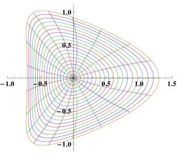
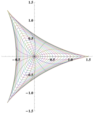
Figure 1. The images of $\mathbb{D}$ under the mappings $F_{1}(z)=z+\frac{1}{10}z^{2}+\frac{1}{5}\overline{z^{2}}$ (left) and $F_{2}(z)=z+\frac{1}{101}z^{2}+\frac{49}{101}\overline{z^{2}}$ (right).

Example 2.

Let $F_{2}(z)=z+\frac{1}{101}z^{2}+\frac{49}{101}\overline{z^{2}}$. Then $F_{2}\in HS_{1}^{0}(\frac{1}{100})$ is a univalent, sense preserving polyharmonic mapping. In particular, $F_{2}$ maps $\mathbb{D}$ onto a domain starlike w.r.t. the origin, and it maps the disk $\mathbb{D}_{r}$, where $r\leq\frac{1}{2}$, onto a convex domain. See Figure 1.

4. Extremal points

First, we determine the distortion bounds for mappings in $HS_{p}(\lambda)$.

Lemma 1.

Suppose that $F\in HS_{p}(\lambda)$. Then the following statements hold:

$(1)$ For $0\leq\lambda\leq\frac{1}{2}$,

$$(1-|b_{1,1}|)|z|-\frac{1-|b_{1,1}|}{2(1+\lambda)}|z|^{2}\leq|F(z)|\leq(1+|b_{1,1}|)|z|+\frac{1-|b_{1,1}|}{2(1+\lambda)}|z|^{2}.$$

Equalities are obtained by the mappings

$$F(z)=z+|b_{1,1}|e^{i\mu}\overline{z}+\frac{1-|b_{1,1}|}{2(1+\lambda)}e^{i\nu}z^{2},$$

for properly chosen real $\mu$ and $\nu$;

$(2)$ For $\frac{1}{2}<\lambda\leq 1$,

$$|F(z)\leq(1+|b_{1,1}|)|z|+\frac{1-|b_{1,1}|-3(|a_{1,2}|+|b_{1,2}|)}{2(1+\lambda)}|z|^{2}+(|a_{1,2}|+|b_{1,2}|)|z|^{3}$$

and

$$|F(z)|\geq(1-|b_{1,1}|)|z|-\frac{1-|b_{1,1}|-3(|a_{1,2}|+|b_{1,2}|)}{2(1+\lambda)}|z|^{2}-(|a_{1,2}|+|b_{1,2}|)|z|^{3}.$$

Equalities are obtained by the mappings

$$F(z)=z+|b_{1,1}|e^{i\eta}\overline{z}+\frac{1-|b_{1,1}|-3(|a_{1,2}|+|b_{1,2}|)}{2(1+\lambda)}e^{i\varphi}z^{2}+(|a_{1,2}|+|b_{1,2}|)e^{i\psi}z|z|^{2},$$

for properly chosen real $\eta$, $\varphi$ and $\psi$.

Proof. Let $F\in HS_{p}(\lambda)$, where $\lambda\in[0,1]$. By (2.1), we have

$$|F(z)|\leq(1+|b_{1,1}|)|z|+\left(\sum_{k=1}^{p}\sum_{n=2}^{\infty}(|a_{n,k}|+|b_{n,k}|)+\sum_{k=2}^{p}(|a_{1,k}|+|b_{1,k}|)\right)|z|^{2}.$$

For $0\leq\lambda\leq\frac{1}{2}$, we have

(4.1) $$2(1+\lambda)\leq 2k-1,$$

where $k\in\{2,\cdots,p\}$, and

(4.2) $$2(1+\lambda)\leq 2(k-1)+n(\lambda n+1-\lambda),$$

where $k\in\{1,\cdots,p\}$ and $n\geq 2$. Then (4.1), (4.2) and (2.4) give

$$\sum_{k=1}^{p}\sum_{n=2}^{\infty}(|a_{n,k}|+|b_{n,k}|)+\sum_{k=2}^{p}(|a_{1,k}|+|b_{1,k}|)$$

$$\leq \frac{1}{2(1+\lambda)}\Big{(}1-|b_{1,1}|-\sum_{k=1}^{p}\sum_{n=2}^{\infty}\big{(}2(k-1)+n(\lambda n+1-\lambda)-2(1+\lambda)\big{)}(|a_{n,k}|+|b_{n,k}|)$$

$$-\sum_{k=2}^{p}\big{(}(2k-1)-2(1+\lambda)\big{)}(|a_{1,k}|+|b_{1,k}|)\Big{)},$$

so

$$(1-|b_{1,1}|)|z|-\frac{1-|b_{1,1}|}{2(1+\lambda)}|z|^{2}\leq|F(z)|\leq(1+|b_{1,1}|)|z|+\frac{1-|b_{1,1}|}{2(1+\lambda)}|z|^{2}.$$

By (2.1), we obtain

$$|F(z)| \leq (1+|b_{1,1}|)|z|+\left(\sum_{k=1}^{p}\sum_{n=2}^{\infty}(|a_{n,k}|+|b_{n,k}|)+\sum_{k=3}^{p}(|a_{1,k}|+|b_{1,k}|)\right)|z|^{2}$$

$$+ (|a_{1,2}|+|b_{1,2}|)|z|^{3}.$$

For $\frac{1}{2}<\lambda\leq 1$, we have

(4.3) $$2(1+\lambda)\leq 2k-1,$$

where $k\in\{3,\cdots,p\}$, and

(4.4) $$2(1+\lambda)\leq 2(k-1)+n(\lambda n+1-\lambda),$$

where $k\in\{1,\cdots,p\},\;n\geq 2$. Then (4.3), (4.4) and (2.4) imply

$$\sum_{k=1}^{p}\sum_{n=2}^{\infty}(|a_{n,k}|+|b_{n,k}|)+\sum_{k=3}^{p}(|a_{1,k}|+|b_{1,k}|)$$

$$\leq \frac{1}{2(1+\lambda)}\Big{(}1-|b_{1,1}|-\sum_{k=1}^{p}\sum_{n=2}^{\infty}\big{(}2(k-1)+n(\lambda n+1-\lambda)-2(1+\lambda)\big{)}(|a_{n,k}|+|b_{n,k}|)$$

$$-\sum_{k=3}^{p}\big{(}2k-1-2(1+\lambda)\big{)}(|a_{1,k}|+|b_{1,k}|)-3(|a_{1,2}|+|b_{1,2}|)\Big{)}.$$

Then

$$|F(z)|\geq(1-|b_{1,1}|)|z|-\frac{1-|b_{1,1}|-3(|a_{1,2}|+|b_{1,2}|)}{2(1+\lambda)}|z|^{2}-(|a_{1,2}|+|b_{1,2}|)|z|^{3}$$

and

$$|F(z)|\leq(1+|b_{1,1}|)|z|+\frac{1-|b_{1,1}|-3(|a_{1,2}|+|b_{1,2}|)}{2(1+\lambda)}|z|^{2}+(|a_{1,2}|+|b_{1,2}|)|z|^{3}.$$

The proof of this lemma is complete.∎

Remark 1.

Suppose that $F\in HS_{p}(\lambda)$ is of the form

$$F(z)=\sum_{k=1}^{p}|z|^{2(k-1)}G_{k}(z)=\sum_{k=1}^{p}|z|^{2(k-1)}\sum_{n=1}^{\infty}\left(a_{n,k}z^{n}+\overline{b_{n,k}}\overline{z^{n}}\right).$$

Then for each $k\in\{1,\cdots,p\}$,

$$|G_{k}(z)|\leq(|a_{1,k}|+|b_{1,k}|)|z|+\frac{1-|b_{1,1}|}{2(1+\lambda)}|z|^{2}.$$

Lemma 2.

The family $HS_{p}(\lambda)$ is closed under convex combinations.

Proof. Suppose $F_{i}\in HS_{p}(\lambda)$ and $t_{i}\in[0,1]$ with $\sum_{i=1}^{\infty}t_{i}=1$. Let

$$F_{i}(z)=\sum_{k=1}^{p}|z|^{2(k-1)}\sum_{n=1}^{\infty}(a^{(i)}_{n,k}z^{n}+\overline{b^{(i)}_{n,k}}\overline{z^{n}}).$$

By Lemma 1, there exists a constant $M$ such that $|F_{i}(z)|\leq M$ for all $i=1,\cdots,p$. It follows that $\sum_{i=1}^{\infty}t_{i}F_{i}(z)$ is absolutely and uniformly convergent, and by Remark 1, the mapping $\sum_{i=1}^{\infty}t_{i}F_{i}(z)$ is polyharmonic. Since $\sum_{i=1}^{\infty}t_{i}F_{i}(z)$ is absolutely and uniformly convergent, we have

$$\sum_{i=1}^{\infty}t_{i}F_{i}(z) =\sum_{i=1}^{\infty}t_{i}\sum_{k=1}^{p}|z|^{2(k-1)}\left(\sum_{n=1}^{\infty}a^{(i)}_{n,k}z^{n}+\sum_{n=1}^{\infty}\overline{b^{(i)}_{n,k}}\overline{z^{n}}\right)$$

$$=\sum_{k=1}^{p}|z|^{2(k-1)}\left(\sum_{n=1}^{\infty}\sum_{i=1}^{\infty}t_{i}a^{(i)}_{n,k}z^{n}+\sum_{n=1}^{\infty}\sum_{i=1}^{\infty}t_{i}\overline{b^{(i)}_{n,k}}\overline{z^{n}}\right).$$

By (2.4), we get

(4.5) $$\sum_{k=1}^{p}\sum_{n=1}^{\infty}\big{(}2(k-1)+n(\lambda n+1-\lambda)\big{)}\left(\left|\sum_{i=1}^{\infty}t_{i}a^{(i)}_{n,k}\right|+\left|\sum_{i=1}^{\infty}t_{i}b^{(i)}_{n,k}\right|\right)$$

$$\leq\sum_{i=1}^{\infty}t_{i}\left(\sum_{k=1}^{p}\sum_{n=1}^{\infty}\big{(}2(k-1)+n(\lambda n+1-\lambda)\big{)}(|a^{(i)}_{n,k}|+|b^{(i)}_{n,k}|)\right)\leq 2.$$

It follows from

$$1\leq\sum_{k=1}^{p}(2k-1)\left(\left|\sum_{i=1}^{\infty}t_{i}a^{(i)}_{1,k}\right|+\left|\sum_{i=1}^{\infty}t_{i}b^{(i)}_{1,k}\right|\right)<2$$

and (4.5) that $\sum_{i=1}^{\infty}t_{i}F_{i}\in HS_{p}(\lambda)$. ∎

From Lemma 1, we see that the class $HS_{p}(\lambda)$ is uniformly bounded, and hence normal. Lemma 2 implies that $HS^{0}_{p}(\lambda)$ is also compact and convex. Then there exists a non-empty set of extremal points in $HS_{p}^{0}(\lambda)$.

Theorem 2.

The extremal points of $HS_{p}^{0}(\lambda)$ are the mappings of the following form:

$$F_{k}(z)=z+|z|^{2(k-1)}a_{n,k}z^{n}\;\text{or}\;F^{*}_{k}(z)=z+|z|^{2(k-1)}\overline{b_{m,k}}\overline{z^{m}},$$

where

$$|a_{n,k}|=\frac{1}{2(k-1)+n(\lambda n+1-\lambda)},\;\;\text{for}\;n\geq 2,\;k\in\{1,\cdots,p\},$$

and

$$|b_{m,k}|=\frac{1}{2(k-1)+m(\lambda m+1-\lambda)},\;\;\text{for}\;m\geq 2,\;k\in\{1,\cdots,p\}.$$

Proof. Assume that $F$ is an extremal point of $HS_{p}^{0}(\lambda)$, of the form $(\ref{eq1.1})$. Suppose that the coefficients of $F$ satisfy the following:

$$\sum_{k=1}^{p}\sum_{n=2}^{\infty}\big{(}2(k-1)+n(\lambda n+1-\lambda)\big{)}(|a_{n,k}|+|b_{n,k}|)<1.$$

If all coefficients $a_{n,k}$ $(n\geq 2)$ and $b_{n,k}$ $(n\geq 2)$ are equal to $0$, we let

$$F_{1}(z)=z+\frac{1}{2(1+\lambda)}z^{2}\;\text{and}\;F_{2}(z)=z-\frac{1}{2(1+\lambda)}z^{2}.$$

Then $F_{1}$ and $F_{2}$ are in $HS_{p}^{0}(\lambda)$ and $F=\frac{1}{2}(F_{1}+F_{2})$. This is a contradiction, showing that there is a coefficient, say $a_{n_{0},k_{0}}$ or $b_{n_{0},k_{0}}$, of $F$ which is nonzero. Without loss of generality, we may further assume that $a_{n_{0},k_{0}}\neq 0$.

For $\gamma>0$ small enough, choosing $x\in\mathbb{C}$ with $|x|=1$ properly and replacing $a_{n_{0},k_{0}}$ by $a_{n_{0},k_{0}}-\gamma x$ and $a_{n_{0},k_{0}}+\gamma x$, respectively, we obtain two mappings $F_{3}$ and $F_{4}$ such that both $F_{3}$ and $F_{4}$ are in $HS_{p}^{0}(\lambda)$. Obviously, $F=\frac{1}{2}(F_{3}+F_{4})$. Hence the coefficients of $F$ must satisfy the following equality:

$$\sum_{k=1}^{p}\sum_{n=2}^{\infty}\big{(}2(k-1)+n(\lambda n+1-\lambda)\big{)}(|a_{n,k}|+|b_{n,k}|)=1.$$

Suppose that there exists at least two coefficients, say, $a_{q_{1},k_{1}}$ and $b_{q_{2},k_{2}}$ or $a_{q_{1},k_{1}}$ and $a_{q_{2},k_{2}}$ or $b_{q_{1},k_{1}}$ and $b_{q_{2},k_{2}}$, which are not equal to 0, where $q_{1}$, $q_{2}\geq 2$. Without loss of generality, we assume the first case. Choosing $\gamma>0$ small enough and $x\in\mathbb{C}$, $y\in\mathbb{C}$ with $|x|=|y|=1$ properly, leaving all coefficients of $F$ but $a_{q_{1},k_{1}}$ and $b_{q_{2},k_{2}}$ unchanged and replacing $a_{q_{1},k_{1}},b_{q_{2},k_{2}}$ by

$$a_{q_{1},k_{1}}+\frac{\gamma x}{2(k_{1}-1)+q_{1}(\lambda q_{1}+1-\lambda)}\;\;\text{and}\;\;b_{q_{2},k_{2}}-\frac{\gamma y}{2(k_{2}-1)+q_{2}(\lambda q_{2}+1-\lambda)},$$

or

$$a_{q_{1},k_{1}}-\frac{\gamma x}{2(k_{1}-1)+q_{1}(\lambda q_{1}+1-\lambda)}\;\;\text{and}\;\;b_{q_{2},k_{2}}+\frac{\gamma y}{2(k_{2}-1)+q_{2}(\lambda q_{2}+1-\lambda)},$$

respectively, we obtain two mappings $F_{5}$ and $F_{6}$ such that $F_{5}$ and $F_{6}$ are in $HS_{p}^{0}(\lambda)$. Obviously, $F=\frac{1}{2}(F_{5}+F_{6})$. This shows that any extremal point $F\in HS_{p}^{0}(\lambda)$ must have the form $F_{k}(z)=z+|z|^{2(k-1)}a_{n,k}z^{n}$ or $F^{*}_{k}(z)=z+|z|^{2(k-1)}\overline{b_{m,k}}\overline{z^{m}}$, where

$$|a_{n,k}|=\frac{1}{2(k-1)+n(\lambda n+1-\lambda)},\;\;\text{for}\;n\geq 2,\;k\in\{1,\cdots,p\},$$

and

$$|b_{m,k}|=\frac{1}{2(k-1)+m(\lambda m+1-\lambda)},\;\;\text{for}\;m\geq 2,\;k\in\{1,\cdots,p\}.$$

Now we are ready to prove that for any $F\in HS_{p}^{0}(\lambda)$ with the above form must be an extremal point of $HS_{p}^{0}(\lambda)$. It suffices to prove the case of $F_{k}$, since the proof for the case of $F^{*}_{k}$ is similar.

Suppose there exist two mappings $F_{7}$ and $F_{8}\in HS_{p}^{0}(\lambda)$ such that $F_{k}=tF_{7}+(1-t)F_{8}\;(0<t<1).$ For $q=7,8$, let

$$F_{q}(z)=\sum_{k=1}^{p}|z|^{2(k-1)}\sum_{n=1}^{\infty}(a^{(q)}_{n,k}z^{n}+\overline{b^{(q)}_{n,k}}\overline{z^{n}}).$$

Then

(4.6) $$|ta_{n,k}^{(7)}+(1-t)a_{n,k}^{(8)}|=|a_{n,k}|=\frac{1}{2(k-1)+n(\lambda n+1-\lambda)}.$$

Since all coefficients of $F_{q}\;(q=7,8)$ satisfy, for $n\geq 2$ and $k\in\{1,\cdots,p\}$,

$$|a_{n,k}^{(q)}|\leq\frac{1}{2(k-1)+n(\lambda n+1-\lambda)},\quad|b_{n,k}^{(q)}|\leq\frac{1}{2(k-1)+n(\lambda n+1-\lambda)},$$

(4.6) implies $a_{n,k}^{(7)}=a_{n,k}^{(8)}$, and all other coefficients of $F_{7}$ and $F_{8}$ are equal to $0$. Thus $F_{k}=F_{7}=F_{8}$, which shows that $F_{k}$ is an extremal point of $HS_{p}^{0}(\lambda).$ ∎

5. Convolutions and neighborhoods

Let $C_{H}^{0}$ denote the class of harmonic univalent, convex mappings $F$ of the form (1.1) with $b_{1}=0$. It is known [10] that the below sharp inequalities hold:

$$2|a_{n}|\leq n+1,\;\;2|b_{n}|\leq n-1.$$

It follows from [10, Theorems $5.14$] that if $H$ and $G$ are in $C_{H}^{0}$, then $H\ast G$ (or $H\diamond G$) is sometime not convex, but it may be univalent or even convex if one of the mappings $H$ and $F$ satisfies some additional conditions. In this section, we consider convolutions of harmonic mappings $F\in HS_{1}^{0}(\lambda)$ and $H\in C^{0}_{H}$.

Theorem 3.

Suppose that $H(z)=z+\sum_{n=2}^{\infty}(A_{n}z^{n}+\overline{B_{n}}\overline{z^{n}})\in C_{H}^{0}$ and $F\in HS_{1}^{0}(\lambda)$. Then for $\frac{1}{2}\leq\lambda\leq 1$, the convolution $F\ast H$ is univalent and starlike, and the integral convolution $F\diamond H$ is convex.

Proof. If $F(z)=z+\sum_{n=2}^{\infty}(a_{n}z^{n}+\overline{b_{n}}\overline{z^{n}})\in HS_{1}^{0}(\lambda)$, then for $F\ast H$, we obtain

$$\sum_{n=2}^{\infty}n(|a_{n}A_{n}|+|b_{n}B_{n}|)\leq \sum_{n=2}^{\infty}n\left(\frac{n+1}{2}|a_{n}|+\frac{n-1}{2}|b_{n}|\right)$$

$$\leq \sum_{n=2}^{\infty}n(\lambda n+1-\lambda)(|a_{n}|+|b_{n}|)\leq 1.$$

Hence $(F\ast H)\in HS^{0}$. The transformations

$$\int_{0}^{1}\frac{F(z)\ast H(tz)}{t}dt=(F\diamond H)(z)$$

now show that $(F\diamond H)\in HC^{0}$. By Theorem A, the result follows. ∎

Remark 2.

The proof of the Theorem 3 does not generalize to polyharmonic mappings, when $p\geq 2$. For example, let $p=2$, and write

$$H(z)=z+\sum_{k=1}^{2}|z|^{2(k-1)}\sum_{n=2}^{\infty}(A_{n,k}z^{n}+\overline{B_{n,k}}\overline{z^{n}})$$

and

$$F(z)=z+\sum_{k=1}^{2}|z|^{2(k-1)}\sum_{n=2}^{\infty}(a_{n,k}z^{n}+\overline{b_{n,k}}\overline{z^{n}}).$$

Suppose that $|A_{n,k}|\leq\frac{n+1}{2}$, $|B_{n,k}|\leq\frac{n-1}{2}$ and $F\in HS_{2}^{0}(\lambda)$. Then for $\lambda=1$, the convolution $F\ast H$ is univalent and starlike but it is not clear if this is true for $\frac{1}{2}\leq\lambda<1$. However, the integral convolution $F\diamond H$ is convex for $\frac{1}{2}\leq\lambda\leq 1$.

Example 3.

Let $H(z)$=$\rm{Re}$$\big{\{}\frac{z}{1-z}\big{\}}+i$$\rm{Im}$$\big{\{}\frac{z}{(1-z)^{2}}\big{\}}\in$$C_{H}^{0}$. Then $H(z)$ maps $\mathbb{D}$ onto the half-plane $\rm{Re}$$\{w\}>\frac{1}{2}$, and let $F(z)=z+\frac{1}{10}z^{2}+\frac{1}{5}\overline{z^{2}}\in HS^{0}_{1}(\frac{2}{3})$. Then the convolution $F\ast H$ is univalent and starlike, and the integral convolution $F\diamond H$ is convex (see Figure 2).

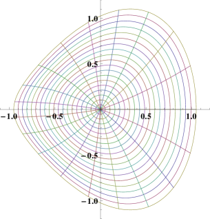
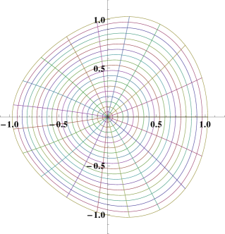
Figure 2. The images of $\mathbb{D}$ under the mappings $(F\ast H)(z)=z+\frac{3}{20}z^{2}-\frac{1}{10}\overline{z^{2}}$ (left) and $(F\diamond H)(z)=z+\frac{3}{40}z^{2}-\frac{1}{20}\overline{z^{2}}$ (right).

Finally, we are going to prove the existence of neighborhoods for mappings in the class $HS_{p}(\lambda)$.

Theorem 4.

Assume that $\lambda\in(0,1]$ and $F\in HS_{p}(\lambda)$. If

$$\delta\leq\frac{\lambda}{p+\lambda}\left(2-\sum_{k=1}^{p}(2k-1)(|a_{1,k}|+|b_{1,k}|)\right),$$

then $N_{\delta}(F)\subset HS_{p}$.

Proof. Let $H(z)=\sum_{k=1}^{p}|z|^{2(k-1)}\sum_{n=1}^{\infty}(A_{n,k}z^{n}+\overline{B_{n,k}}\overline{z}^{n})\in N_{\delta}(F)$. Then

$$\sum_{k=1}^{p}\sum_{n=2}^{\infty}\big{(}2(k-1)+n\big{)}(|A_{n,k}|+|B_{n,k}|)+\sum_{k=2}^{p}(2k-1)(|A_{1,k}|+|B_{1,k}|)+|B_{1,1}|$$

$$\leq \sum_{k=1}^{p}\sum_{n=2}^{\infty}\big{(}2(k-1)+n\big{)}(|A_{n,k}-a_{n,k}|+|B_{n,k}-b_{n,k}|)$$

$$+\sum_{k=2}^{p}(2k-1)(|A_{1,k}-a_{1,k}|+|B_{1,k}-b_{1,k}|)+|B_{1,1}-b_{1,1}|$$

$$+\sum_{k=1}^{p}\sum_{n=2}^{\infty}\big{(}2(k-1)+n\big{)}(|a_{n,k}|+|b_{n,k}|)+\sum_{k=2}^{p}(2k-1)(|a_{1,k}|+|b_{1,k}|)+|b_{1,1}|$$

$$\leq \delta+\sum_{k=1}^{p}\sum_{n=2}^{\infty}\big{(}2(k-1)+n\big{)}(|a_{n,k}|+|b_{n,k}|)+\sum_{k=2}^{p}(2k-1)(|a_{1,k}|+|b_{1,k}|)+|b_{1,1}|$$

$$\leq \delta+\frac{p}{p+\lambda}\sum_{k=1}^{p}\sum_{n=2}^{\infty}\big{(}2(k-1)+n(\lambda n+1-\lambda)\big{)}(|a_{n,k}|+|b_{n,k}|)$$

$$+\sum_{k=2}^{p}(2k-1)(|a_{1,k}|+|b_{1,k}|)+|b_{1,1}|$$

$$\leq \delta+\frac{p-\lambda}{p+\lambda}+\frac{\lambda}{p+\lambda}\sum_{k=1}^{p}(2k-1)(|a_{1,k}|+|b_{1,k}|)<1.$$

Hence, $H\in HS_{p}$. ∎

References

[1]
[2]Z. Abdulhadi and Y. Abu Muhanna, Landau’s theorem for biharmonic mappings.
J. Math. Anal. Appl.338 (2008), 705–709.
[3]Z. Abdulhadi, Y. Abu Muhanna and S. Khuri, On univalent solutions of the
biharmonic equation. J. Inequal. Appl.5 (2005), 469–478.
[4]Z. Abdulhadi, Y. Abu Muhanna and S. Khuri, On some properties of solutions
of the biharmonic equation. Appl. Math. Comput.117 (2006), 346–351.
[5]Y. Avci and E. Złotkiewicz, On harmonic univalent mappings. Ann. Univ. Mariae Curie-Skłodowska (Sect A)44 (1990), 1–7.
[6]Sh. Chen, S. Ponnusamy and X. Wang, Landau’s theorem for certain biharmonic mappings,
Appl. Math. Comput.208 (2009), 427–433.
[7]Sh. Chen, S. Ponnusamy and X. Wang, Compositions of harmonic mappings and biharmonic
mappings. Bull. Belg. Math. Soc. Simon Stevin.17 (2010), 693–704.
[8]Sh. Chen, S. Ponnusamy and X. Wang, Bloch constant and Landau’s theorem
for planar -harmonic mappings. J. Math. Anal. Appl.373 (2011), 102–110.
[9]J. Chen and X. Wang, On certain classes of biharmonic mappings
defined by convolution. Abstract and Applied Analysis.
2012, Article ID 379130, 10 pages. doi:10.1155/2012/379130
[10]J. G. Clunie and T. Sheil-Small, Harmonic univalent functions.
Ann. Acad. Sci. Fenn. Ser. A. I.9 (1984), 3–25.
[11]P. Duren, Univalent functions. Spring-Verlag, New York 1983.
[12]P. Duren, Harmonic mappings in the plane. Cambridge University Press, Cambridge 2004.
[13]M. Fait, J. Krzyż and J. Zygmunt,
Explicit quasiconformal extensions for some classes of univalent functions.
Comment. Math. Helv.51 (1976), 279–285.
[14]A. W. Goodman, Univalent functions and nonanalytic curves, Proc. Amer. Math. Soc.8 (1957), 588–601.
[15]J. Happel and H. Brenner,
Low Reynolds Number Hydrodynamics with Special Applications to Particulate
Media. Prentice-Hall, Englewood Cliffs, NJ, USA, 1965.
[16]S. A. Khuri, Biorthogonal series solution of Stokes flow problems in sectorial regions.
SIAM J. Appl. Math.56 (1996), 19–39.
[17]W. E. Langlois, Slow Viscous Flow. Macmillan, New York, NY, USA, 1964.
[18]J. Qiao and X. Wang, On -harmonic univalent mappings (in Chinese). Acta Math. Sci.32A (2012), 588–600.
[19]C. Pommerenke, Univalent functions. Vandenhoeck and Ruprecht, Götting-en, 1975.
[20]S. Ruscheweyh, Neighborhoods of univalent functions. Proc. Amer. Math. Soc.18 (1981), 521–528.