Parallel Unsmoothed Aggregation Algebraic Multigrid Algorithms on GPUs

Abstract.

We design and implement a parallel algebraic multigrid method for isotropic graph Laplacian problems on multicore Graphical Processing Units (GPUs). The proposed AMG method is based on the aggregation framework. The setup phase of the algorithm uses a parallel maximal independent set algorithm in forming aggregates and the resulting coarse level hierarchy is then used in a K-cycle iteration solve phase with a $\ell^{1}$-Jacobi smoother. Numerical tests of a parallel implementation of the method for graphics processors are presented to demonstrate its effectiveness.

1. Introduction

We consider development of a multilevel iterative solver for large-scale sparse linear systems corresponding to graph Laplacian problems for graphs with balanced vertex degrees. A typical example is furnished by the matrices corresponding to the (finite difference)/(finite volume)/(finite element) discretizations of scalar elliptic equation with mildly varying coefficients on unstructured grids.

Multigrid (MG) methods have been shown to be very efficient iterative solvers for graph Laplacian problems and numerous parallel MG solvers have been developed for such systems. Our aim here is to design an algebraic multigrid (AMG) method for solving the graph Laplacian system and discuss the implementation of such methods on multi-processor parallel architectures, with an emphasis on implementation on Graphical Processing Units (GPUs).

The programming environment which we use in this paper is the Compute Unified Device Architecture (CUDA) toolkit introduced in 2006 by NVIDIA which provides a framework for programming on GPUs. Using this framework in the last 5 years several variants of Geometric Multigrid (GMG) methods have been implemented on GPUs [17, 6, 16, 18, 14, 13] and a high level of parallel performance for the GMG algorithms on CUDA-enabled GPUs has been demonstrated in these works.

On the other hand, designing AMG methods for massively parallel heterogenous computing platforms, e.g., for clusters of GPUs, is very challenging mainly due to the sequential nature of the coarsening processes (setup phase) used in AMG methods. In most AMG algorithms, coarse-grid points or basis are selected sequentially using graph theoretical tools (such as maximal independent sets and graph partitioning algorithms). Although extensive research has been devoted to improving the performance of parallel coarsening algorithms, leading to notable improvements on CPU architectures [9, 28, 27, 21, 11, 8, 22, 28], on a single GPU [3, 26, 19], and on multiple GPUs [12], the setup phase is still considered a bottleneck in parallel AMG methods. We mention the work in [3], where a smoothed aggregation setup is developed in CUDA for GPUs.

In this paper, we describe a parallel AMG method based on the un-smoothed aggregation AMG (UA-AMG) method. The setup algorithm we develop and implement has several notable design features. A key feature of our parallel aggregation algorithm is that it first chooses coarse vertices using a parallel maximal independent set algorithm [11] and then forms aggregates by grouping coarse level vertices with their neighboring fine level vertices, which, in turn, avoids ambiguity in choosing fine level vertices to form aggregates. Such a design eliminates both the memory write conflicts and conforms to the CUDA programming model. The triple matrix product needed to compute the coarse-level matrix (a main bottleneck in parallel AMG setup algorithms) simplifies significantly in the UA-AMG setting, reducing to summations of entries in the matrix on the finer level. The parallel reduction sums available in CUDA are quite an efficient tool for this task during the AMG setup phase. Additionally, the UA-AMG setup typically leads to low grid and operator complexities.

In the solve phase of the proposed algorithm, a K-cycle [29, 1, 2] is used to accelerate the convergence rate of the multilevel UA-AMG method. Such multilevel method optimizes the coarse grid correction and results in an approximate two-level method. Two parallel relaxation schemes considered in our AMG implementation are a damped Jacobi smoother and a parameter free $\ell^{1}$-Jacobi smoother introduced in [25] and its weighted version in [7]. To further accelerate the convergence rate of the resulting K-cycle method we apply it as a preconditioner to a nonlinear conjugate gradient method.

The remainder of the paper is organized as follows. In Section 2, we review the UA-AMG method. Then, in Section 3, a parallel graph aggregation method is introduced, which is our main contribution. The parallelization of the solve phase is discussed in Section 4. In Section 5, we present some numerical results to demonstrate the efficiency of the parallel UA-AMG method.

2. Unsmoothed Aggregation AMG

The linear system of interest has as coefficient matrix the graph Laplacian corresponding to an undirected connected graph $\mathcal{G}=(\mathcal{V},\mathcal{E})$. Here, $\mathcal{V}$ denotes the set of vertices and $\mathcal{E}$ denotes the set of edges of $\mathcal{G}$. We set $n=|\mathcal{V}|$ (cardinality of $\mathcal{V}$). By $(\cdot,\cdot)$ we denote the inner product in $\ell^{2}({\rm I\!R}^{n})$ and the superscript $t$ denotes the adjoint with respect to this inner product. The graph Laplacian $A:{\rm I\!R}^{n}\mapsto{\rm I\!R}^{n}$ is then defined via the following bilinear form

$$(Au,v)=\sum_{k=(i,j)\in\mathcal{E}}\omega_{ij}(u_{i}-u_{j})(v_{i}-v_{j})+\sum_{j\in\mathcal{S}}\omega^{D}_{j}u_{j}v_{j},\quad\mathcal{S}\subset\mathcal{V}.$$

We assume that the weights $\omega_{ij}$, and $\omega^{D}_{j}$ are strictly positive for all $i$ and $j$. The first summation is over the set of edges $\mathcal{E}$ (over $k\in\mathcal{E}$ connecting the vertices $i$ and $j$), and $u_{i}$ and $u_{j}$ are the $i$-th and $j$-th coordinate of the vector $u\in{\rm I\!R}^{n}$, respectively. We also assume that the subset of vertices $\mathcal{S}$ is such that the resulting matrix $A$ is symmetric positive definite (SPD). If the graph is connected $\mathcal{S}$ could contain only one vertex and $A$ will be SPD. For matrices corresponding to the discretization scalar elliptic equation on unstructured grids $\mathcal{S}$ is the set of vertices near (one edge away from) the boundary of the computational domain. The linear system of interest is then

(2.1) $$Au=f.$$

With this system of equation we associate a multilevel hierarchy which consists of spaces $V_{0}\subset V_{1}\subset\ldots\subset V_{L}={\rm I\!R}^{n}$, each of the spaces is defined as the range of interpolation/prolongation operator $P_{l-1}^{l}:{\rm I\!R}^{n_{l-1}}\mapsto V_{l}$ with $\operatorname{Range}(P_{l-1}^{l})=V_{l-1}$.

Given the $l$-th level matrix $A_{l}\in\mathbb{R}^{n_{l}\times n_{l}}$, the aggregation-based prolongation matrix $P_{l-1}^{l}$ is defined in terms of a non-overlapping partition of the $n_{l}$ unknowns at level $l$ into the $n_{l-1}$ nonempty disjoint sets $G_{j}^{l}$, $j=1,\dots,n_{l-1}$, called aggregates. An algorithm for choosing such aggregates is presented in the next section. The prolongation $P_{l-1}^{l}$ is the $n_{l}\times n_{l-1}$ matrix with columns defined by partitioning the constant vector, $\mathbbm{1}=(1,\ldots,1)^{t}$, with respect to the aggregates:

(2.2) $$(P_{l-1}^{l})_{ij}=\begin{cases}1&\text{if}\ i\in G_{j}^{l}\\ 0&\text{otherwise}\end{cases}\quad i=1,\dots,n_{l},\quad j=1,\dots,n_{l-1}.$$

The resulting coarse-level matrix $A_{l-1}\in\mathbb{R}^{n_{l-1}\times n_{l-1}}$ is then defined by the so called “triple matrix product”, namely,

(2.3) $$A_{l-1}=(P_{l-1}^{l})^{t}A_{l}(P_{l-1}^{l}).$$

Note that since we consider UA-AMG, the interpolation operators are boolean matrices such that the entries in the coarse-grid matrix $A_{l-1}$ can be obtained from a simple summation process:

(2.4) $$(A_{l-1})_{ij}=\sum_{s\in G_{i}}\sum_{t\in G_{j}}a_{st},\quad i,j=1,2,\cdots,n_{l-1}.$$

Thus, the triple matrix product, typically the costly procedure in an AMG setup, simplifies significantly for UA-AMG to reduction sums.

We now introduce a general UA-AMG method (see Algorithm 1) and in the subsequent sections we describe the implementation of each of the components of Algorithm 1 for GPUs.

Algorithm 1 UA-AMG

3. The Setup Phase

Consider the system of linear equations (2.1) corresponding to an unweighted graph $\mathcal{G}=\{\mathcal{V},\mathcal{E}\}$ partitioned into two subgraphs $\mathcal{G}_{k}=\{\mathcal{V}_{k},\mathcal{E}_{k}\},k=1,2$. Further assume that the two subgraphs are stored on separate computes. To implement a Jacobi or Gauss-Seidel smoother for the graph Laplacian equation with respect to $\mathcal{G}$, the communication between the two computers is proportional to the number of edge cuts of such a partitioning, given by

$$|\mathcal{E}\backslash(\mathcal{E}_{1}\cup\mathcal{E}_{2})|.$$

Therefore, a partition corresponding to the minimal edge cut in the graph results in the fastest implementation of such smoothers. This in turn gives a heuristic argument, as also suggested in [24], [23], that when partitioning the graph in subgraphs (aggregates) the subgraphs should have a similar number of vertices and have a small “perimeter.” Such a partitioning can be constructed by choosing any vertex in the graph, naming it as a coarse vertex, and then aggregating it with its neighboring vertices. This heuristic motivates our aggregation method. The algorithm consists of a sequence of two subroutines: first, a parallel maximal independent set algorithm is applied to identify coarse vertices; then a parallel graph aggregation algorithm follows, so that subgraphs (aggregates) centered at the coarse vertices are formed.

In the algorithm, to reduce repeated global memory read access and write conflicts, we impose explicit manual scheduling on data caching and flow control in the implementations of both algorithms; the aim is to achieve the following goals:

1. (Read access coalescence): To store the data that a node uses frequently locally or on a fast connecting neighboring node.

2. (Write conflicting avoidance): To reduce, or eliminate the situation that several nodes need to communicate with a center node simultaneously.

3.1. A Maximal Independent Set Algorithm

The idea behind such algorithm is to simplify the memory coalescence, and design a random aggregation algorithm where there are as many as possible threads loading from a same memory location, while as few as possible threads writing to a same memory location. Therefore, it is natural to have one vertex per thread when choosing the coarse vertices. For vertices that are connected the corresponding processing threads should be wrapped together in a group. By doing so, repeated memory loads from the global memory can be avoided.

However, we also need to ensure that no two coarse vertices compete for a fine level point, because either atomic operations as well as inter-thread communication is costly on a GPU. Therefore, the coarse vertices are chosen in a way that any two of them are of distance 3 or more, which is the same as finding a maximal independent set of vertices for the graph corresponding to $A^{2}$, where $A$ is the graph Laplacian of a given graph $\mathcal{G}$, so that each fine level vertex can be determined independently which coarse vertex it associates with.

Given an undirected unweighted graph $\mathcal{G}=\{\mathcal{V},\mathcal{E}\}$, we first find a set $C$ of coarse vertices such that

(3.1) $$d(i,j)\geq 3,\qquad\forall i,\,j\in C,i\neq j.$$

Here, $d(\cdot,\cdot)$ is the graph distance function defined recursively as

$$d(i,j)=\left\{\begin{matrix}0,&i=j;\\ \displaystyle\min_{k:(i,k)\in E}d(k,j)+1,&i\neq j.\end{matrix}\right.$$

Assume we obtain such set $C$, or even a subset of $C$, we can then form aggregates, by picking up a vertex $i$ in $C$ and defining an aggregate as a set containing $i$ and its neighbors. The condition (3.1) guarantees that two distinct vertices in $C$, do not share any neighbors. The operation of marking the numberings of subgraphs on the fine grid vertices is write conflict free, and the restriction imposed by (3.1) ensures that aggregates can be formed independently, and simultaneously.

The rationale of the independent set algorithm is as follows: First, a random vector $v$ is generated, each component of which corresponds to a vertex in the graph. Then we define the set $C$ as the following:

$$C=\big{\{}i\mid v_{i}>v_{j},\forall j:0<d(i,j)<3\big{\}}.$$

If $C$ is not empty, then such construction results in a collection of vertices in $C$ is of distance 3 or more. Indeed, assume that $d(i,j)<3$ for $i,\,j\in C$, let $v_{i}>v_{j}$. From the definition of the set $C$, we immediately conclude that $i\notin C$. Of course, more caution is needed when $C$ defined above is empty (a situation that may occur depending on the vector $v$). However, this can be remedied, by assuming that the vector $v$ (with random entries) has a global maximum, which is also a local maximum. The $C$ contains at least this vertex. The same algorithm can be applied then recursively to the remaining graph (after this vertex is removed). In practice, $C$ does not contain one but more vertices.

3.2. Parallel Graph Aggregation Algorithm

We here give a description of the parallel aggregation algorithm, running the exact copies of the code on each thread.

Algorithm 2 Parallel Aggregation Algorithm (PAA)

1. Generate a quasi-random number and store it in $v_{i}$, as

   $$v_{i}\longleftarrow\text{quasi\_random}(i);$$

   mark vertex $i$ as “unprocessed”; wait until all threads complete these operations.

2. 1. Goto (2d) if $i$ is marked “processed”, otherwise continue to (2b).

   2. Determine if the vertex $i$ is a coarse vertex, by check if the following is true.

      $$v_{i}>v_{j},\qquad\forall j:(A^{2})_{ij}\neq 0\text{ and $j$ is unprocessed }.$$

      If so, continue to (2c); if not, goto (2d).

   3. Form an aggregate centered at $i$. Let $S_{i}$ be a set of vertices defined as

      $$S_{i}=\big{\{}j\mid v_{i}\geq v_{j},\forall j:(A^{2})_{ij}\neq 0\text{ and $j$ is unprocessed }\big{\}}.$$

      Define a column vector $w$ such that

      $$w_{k}=\left\{\begin{matrix}1,&k\in S_{i};\\ 0,&k\not\in S_{i}.\end{matrix}\right.$$

      Mark vertices $j\in S_{i}$ “processed” and request an atomic operation to update the prolongator $P$ as

      $$P\longleftarrow[P,w]\;.$$

   4. Synchronize all threads (meaning: wait until all threads reach this step).

   5. Stop if $i$ is marked “processed”, otherwise goto step (2a).

Within each pass of the Parallel Aggregation Algorithm (PAA, Algorithm 2), the following two steps are applied to each vertex $i$.

1. Construct a set $C$ which contains coarse vertices.

2. Construct an aggregate for each vertex in $C$.

Note that these two subroutines can be executed in a parallel fashion. Indeed, step (A) does not need to be applied to the whole graph before starting step (B). Even if $C$ is partially completed, any operation in step (B) will not interfere step (A), running on the neighboring vertices and completing the construction of $C$. A problem for this approach is that it usually cannot give a set of aggregates that cover the vertex set $V$ after 1 pass of step (A) and step (B). We thus run several passes and the algorithm terminates when a complete cover is obtained. The number of passes is reduced if we make the set $C$ as large as possible in each pass, therefore the quasi-random vector $v$ needs to have a lot of local maximums. Another heuristic argument is that $C$ needs to be constructed in a way that every coarse vertex has a large number of neighboring vertices. Numerical experiments suggest that the following is a good way of generating the vector $v$ with the desired properties.

(3.2) $$v_{i}\longleftarrow\text{quasi\_random}(i):=d_{i}+\big{(}(i\text{ mod }12)+\text{rand}()\big{)}/12.$$

where $d_{i}$ is the degree of the vertex $i$, and $\text{rand}()$ generates a random number uniformly distributed on the interval $[0,1]$.

3.3. Aggregation Quality Improvements

To improve the quality of the aggregates, we can either impose some constrains during the aggregation procedure (which we call in-line optimization), or introduce a post-process an existing aggregation in order to improve it. One in-line strategy that we use to improve the quality of the aggregation is to limit the number of vertices in an aggregate during the aggregation procedure. However, such limitations may result in a small coarsening ratio. In such case, and numerical results suggest that applying aggregation process twice, which is equivalent to in skipping a level in a multilevel hierarchy, can compensate that.

Our focus is on a post-processing strategy, which we name “rank one optimization”. It uses an a priori estimate to adjust the interface (boundary) of a pair of aggregates, so that the aggregation based two level method, with a fixed smoother, converges fast locally on those two aggregates.

We consider the connected graph formed by a union of aggregates (say a pair of them, which will be the case of interest later), and let $\widehat{n}$ be the dimension of the underlying vector space. Let $\widehat{A}:{\rm I\!R}^{\widehat{n}}\mapsto{\rm I\!R}^{\widehat{n}}$ be a semidefinite weighted graph Laplacian (representing a local sub-problem) and $\widehat{R}$ be a given local smoother. As is usual for semidefinite graph Laplacians, we consider the subspace $\ell^{2}$-orthogonal to the null space of $\widehat{A}$ and we denote it by $V$. The $\ell^{2}$ orthogonal projection on $V$ is denoted here by $\Pi_{V}$. Let $\widehat{S}=I-\widehat{R}\widehat{A}$ be the error propagation operator for the smoother $\widehat{R}$. We consider the two level method whose error propagation matrix is

$$E(V_{c})=E(V_{c};\widehat{S})=(I-Q_{\widehat{A}}(V_{c}))(I-\widehat{R}\widehat{A}).$$

Here $V_{c}\subset V$ is a subspace and $Q_{\widehat{A}}(V_{c})$ is the $\widehat{A}$-orthogonal projection of the elements of $V$ onto the coarse space $V_{c}$. In what follows we use the notation $E(V_{c};\widehat{S})$ when we want to emphasize the dependence on $\widehat{S}$. We note that $Q_{\widehat{A}}(V_{c})$ is well defined on $V$ because $\widehat{A}$ is SPD on $V$ and hence it $(\widehat{A}\cdot,\cdot)$ is an inner product on $V$. We also have that $Q_{\widehat{A}}(V_{c})$ self-adjoint on $V$ and under the assumption $V_{c}\subset V$, we obtain $Q_{\widehat{A}}(V_{c})=\Pi_{V}Q_{\widehat{A}}(V_{c})$ and $\Pi_{V}Q_{\widehat{A}}(V_{c})=Q_{\widehat{A}}(V_{c})\Pi_{V}$. Also, $\widehat{S}_{V}=\Pi_{V}\widehat{S}$ is self-adjoint on $V$ in the $(\widehat{A}\cdot,\cdot)$ inner product iff $\widehat{R}$ is self-adjoint in the $\ell^{2}$-inner product on ${\rm I\!R}^{\widehat{n}}$.

We now introduce the operator $T(V_{c})$ (recall that $V_{c}\subset V$)

$$T(V_{c})=T(V_{c};\widehat{S})=\widehat{S}-E(V_{c})=Q_{\widehat{A}}(V_{c})(I-\widehat{R}\widehat{A})=Q_{\widehat{A}}(V_{c})\widehat{S}.$$

and from the definition of $Q_{\widehat{A}}$ for all $v\in V$ we have

(3.3) $$|E(V_{c})v|_{\widehat{A}}^{2}=|\Pi_{V}E(V_{c})v|_{\widehat{A}}^{2}=|\Pi_{V}\widehat{S}v|_{\widehat{A}}^{2}-|\Pi_{V}T(V_{c})v|_{\widehat{A}}^{2}=|\widehat{S}_{V}v|_{\widehat{A}}^{2}-|T(V_{c})v|_{\widehat{A}}^{2}.$$

We note the following identities which follow directly from the definitions above and the assumption $V_{c}\subset V$:

(3.4) $$|E(V_{c};\widehat{S})|_{\widehat{A}}=|\Pi_{V}E(V_{c};\widehat{S}_{V})|_{\widehat{A}},\quad|T(V_{c};\widehat{S})|_{\widehat{A}}=|\Pi_{V}T(V_{c};\widehat{S}_{V})|_{\widehat{A}}.$$

The relation (3.3) suggests that, in order to minimize the seminorm $|E(V_{c})v|_{\widehat{A}}$ with respect to the coarse space $V_{c}$, we need to make $|T(V_{c})|_{\widehat{A}}$ maximal. The following lemma quantifies this observation and is instrumental in showing how to optimize locally the convergence rate when the subspaces $V_{c}$ are one dimensional. In the statement of the lemma we use $\arg\min$ to denote a subset of minimizers of a given, not necessarily linear, functional $F(x)$ on a space $X$. More precisely, we set

$$y\in\arg\min_{x\in X}{F(x)},\quad\mbox{if and only if},\quad F(y)=\min_{x\in X}{F(x)}.$$

We have similar definition (with obvious changes) for the set $\displaystyle\arg\max_{x\in X}F(x)$.

Lemma 3.1.

Let $\widehat{S}_{V}=\Pi_{V}\widehat{S}$, be the projection of the local smoother on $V$, and $\mathcal{V}_{c}$ be the set of all one dimensional subspaces of $V$. Then we have the following:

(3.5) $$|\widehat{S}_{V}|_{\widehat{A}}=\max_{V_{c}\in\mathcal{V}_{c}}|T(V_{c})|_{\widehat{A}},$$

(3.6) $$\mbox{If $W_{c}\in\displaystyle\arg\max_{V_{c}\in\mathcal{V}_{c}}|T(V_{c})|_{\widehat{A}}$, then $W_{c}\in\displaystyle\arg\min_{V_{c}\in\mathcal{V}_{c}}|E(V_{c})|_{\widehat{A}}$},$$

where $E(V_{c})=(I-Q_{\widehat{A}}(V_{c}))\widehat{S}$ and $T(V_{c})=Q_{\widehat{A}}(V_{c})\widehat{S}$.

Proof. From the identities (3.4) it follows that we can restrict our considerations on $V\subset{\rm I\!R}^{\widehat{n}}$ and that we only need to prove the Lemma with $E(V_{c})=\Pi_{V}E(V_{c};\widehat{S}_{V})$ and $T(V_{c})=\Pi_{V}T(V_{c};\widehat{S}_{V})$. In order to make the presentation more transparent, we denote $|\cdot|=|\cdot|_{\widehat{A}}$, $\Pi=Q_{\widehat{A}}$. Let us mention also that by orthogonality in this proof we mean orthogonality in the $(\widehat{A}\cdot,\cdot)$ inner product on $V$. The proof then proceeds as follows.

Let $\varphi\in V$ be such that $|\widehat{S}_{V}\varphi|=|\widehat{S}_{V}||\varphi|$. We set $W_{c}=\operatorname{span}\{\widehat{S}_{V}\varphi\}$. Note that for such choice of $W_{c}$ we have $\Pi(W_{c})\widehat{S}_{V}\varphi=\widehat{S}_{V}\varphi$ and hence

$$|\widehat{S}_{V}|=\frac{|\widehat{S}_{V}\varphi|}{|\varphi|}=\frac{|T(W_{c})\varphi|}{|\varphi|}\leq|T(W_{c})|.$$

On the other hand, for all $V_{c}\in\mathcal{V}_{c}$ we have $|\Pi(V_{c})|=1$ and we then conclude that

(3.7) $$|T(V_{c})|=|\Pi(V_{c})\widehat{S}_{V}|\leq|\Pi(V_{c})||\widehat{S}_{V}|=|\widehat{S}_{V}|\leq|T(W_{c})|.$$

By taking a maximum on $\mathcal{V}_{c}$ in (3.7), we conclude the following thus prove (3.5).

$$|T(W_{c})|\leq\max_{V_{c}\in\mathcal{V}_{c}}|T(V_{c})|\leq|\widehat{S}_{V}|\leq|T(W_{c})|.$$

To prove (3.6), we observe that for any $W_{c}\in\displaystyle\arg\max_{V_{c}\in\mathcal{V}_{c}}|T(V_{c})|$ the inequalities in (3.7) become equalities and hence

$$|\Pi(W_{c})\widehat{S}_{V}|=|\widehat{S}_{V}|=|\widehat{S}_{V}\Pi(W_{c})|.$$

This implies that $\displaystyle|\widehat{S}_{V}|=\max_{w\in W_{c}}\frac{|\widehat{S}_{V}w|}{|w|}$. It is also clear that $|\widehat{S}_{V}w|=|\widehat{S}_{V}||w|$ for all $w\in W_{c}$, because $W_{c}$ is one dimensional. In addition, since $\widehat{S}_{V}$ is self-adjoint, it follows that $W_{c}$ is the span of the eigenvector of $\widehat{S}_{V}$ with eigenvalue of magnitude $|\widehat{S}_{V}|$. Next, for any $V_{c}\in\mathcal{V}_{c}$ we have

$$|E(V_{c})|=|(I-\Pi(V_{c}))\widehat{S}_{V}|=|\widehat{S}_{V}(I-\Pi(V_{c}))|=\max_{v\in V_{c}^{\perp}}\frac{|\widehat{S}_{V}v|}{|v|}.$$

By the mini-max principle (see [10, pp. 31-35] or [20]) we have that $|E(V_{c})|\geq\sigma_{2}$, where $\sigma_{2}$ is the second largest singular value of $\widehat{S}_{V}$ and with equality holding iff $V_{c}=W_{c}$. This completes the proof. $\blacksquare$

We now move on to consider a pair of aggregates. Let $\widehat{A}$ be the graph Laplacian of a connected positively weighted graph $\widehat{\mathcal{G}}$ which is union of two aggregates $\mathcal{V}_{1}$ and $\mathcal{V}_{2}$. Furthermore, let $\mathbbm{1}_{\mathcal{V}_{1}}$ be the characteristic vector for $\mathcal{V}_{1}$, namely a vector with components equal to $1$ at the vertices of $\mathcal{V}_{1}$ and equal to zero at the vertices of $\mathcal{V}_{2}$. Analogously we have a characteristic vector $\mathbbm{1}_{\mathcal{V}_{2}}$ for $\mathcal{V}_{2}$. Finally, let $V_{c}(\mathcal{V}_{1},\mathcal{V}_{2})$ be the space of vectors that are linear combinations of $\mathbbm{1}_{\mathcal{V}_{1}}$ and $\mathbbm{1}_{\mathcal{V}_{2}}$. More specifically, the subspace $V_{c}$ is defined as

$$V_{c}(\mathcal{V}_{1},\mathcal{V}_{2})=\text{span}\left\{\left(\frac{1}{|\mathcal{V}_{1}|}\mathbbm{1}_{\mathcal{V}_{1}}-\frac{1}{|\mathcal{V}_{2}|}\mathbbm{1}_{\mathcal{V}_{2}}\right)\right\},$$

Let $\mathcal{V}_{c}$ be the set of subspaces defined above for all possible pairs of $\mathcal{V}_{1}$ and $\mathcal{V}_{2}$, such that $\widehat{\mathcal{G}}=\mathcal{V}_{1}\cup\mathcal{V}_{2}$. Note that by the definition above, every pair $(\mathcal{V}_{1},\mathcal{V}_{2})$ gives us a space $V_{c}\in\mathcal{V}_{c}$ which is orthogonal to the null space of $\widehat{A}$, i.e. orthogonal to $\mathbbm{1}=\mathbbm{1}_{\mathcal{V}_{1}}+\mathbbm{1}_{\mathcal{V}_{2}}$.

We now apply the result of Lemma 3.1 and show how to improve locally the quality of the partition (the convergence rate $|E(V_{c})|_{\widehat{A}}$) by reducing the problem of minimizing the $\widehat{A}$-norm of $E(V_{c})$ to the problem of finding the maximum of the $\widehat{A}$-norm of the rank one transformation $T(V_{c})$. Under the assumption that the spaces $V_{c}$ are orthogonal to the null space of $\widehat{A}$ (which they satisfy by construction) from Lemma 3.1 we conclude that the spaces $W_{c}$ which minimize $|E(V_{c})|_{\widehat{A}}$ also maximize $|T(V_{c})|_{\widehat{A}}$.

For the pair of aggregates, $|T(V_{c})|_{\widehat{A}}$ is the largest eigenvalue of $\widehat{S}^{T}AQ_{\widehat{A}}(V_{c})\widehat{S}\widehat{A}^{\dagger}$, where $A^{\dagger}$ is the pseudo inverse of $A$. Clearly, the matrix $\widehat{S}^{T}AQ_{\widehat{A}}(V_{c})\widehat{S}\widehat{A}^{\dagger}$, is also a rank one matrix and hence

$$|T(V_{c})|_{\widehat{A}}=\text{tr}(\widehat{S}^{T}AQ_{\widehat{A}}(V_{c})\widehat{S}\widehat{A}^{\dagger}).$$

During optimization steps, we calculate the trace using the fact that for any rank one matrix $W$ we have

(3.8) $$\text{tr}(W)=\frac{W_{k}^{T}W_{k}}{W_{kk}}=\frac{W_{k}^{T}W_{k}}{e_{k}^{T}W_{k}e_{k}},$$

where $W_{kk}$ is a nonzero diagonal entry (any nonzero diagonal entry) and $W_{k}$ is the $k$-th column of $W$. The formula (3.8) is straightforward to prove if we set $W=uv^{T}$ for two column vectors $u$ and $v$, and also suggests a numerical algorithm. We devise a loop computing $W_{k}=We_{k}$, and $W_{kk}=e_{k}^{T}W_{k}e_{k}$, for $k=1,\dots,m$, where $m$ is the dimension of $W$; The loop is terminated whenever $W_{kk}\neq 0$, and we compute the trace via (3.8) for this $k$. In particular for the examples we have tested, $W=\widehat{S}^{T}\widehat{A}Q_{\widehat{A}}(V_{c})\widehat{S}\widehat{A}^{\dagger}$ is usually a full matrix and we observed that the loop almost always terminated when $k=1$.

The algorithm which traverses all pairs of neighboring aggregates and optimizes their shape is as follows.

Algorithm 3 Subgraph Reshaping Algorithm

1. Input: Two set of vertices, $\mathcal{V}_{1}$ and $\mathcal{V}_{2}$, corresponding to a pair of neighboring subgraphs. Output: Two sets of vertices, $\tilde{\mathcal{V}}_{1}$ and $\tilde{\mathcal{V}}_{2}$ satisfying that

   $$\tilde{\mathcal{V}}_{1}\cup\tilde{\mathcal{V}}_{2}=\mathcal{V}_{1}\cup\mathcal{V}_{2},\qquad\text{ and }\qquad\big{|}|\tilde{\mathcal{V}}_{1}|-|\tilde{\mathcal{V}}_{2}|\big{|}\leq 1,$$

   and the subgraphs corresponding to $\tilde{\mathcal{V}}_{1}$ and $\tilde{\mathcal{V}}_{2}$ are both connected.

2. Let $n=|\tilde{\mathcal{V}}_{1}|+|\tilde{\mathcal{V}}_{2}|$, then compute $m=\lfloor n/2\rfloor$.

3. Run in parallel to generate all partitionings such that the vertices set

   $$\tilde{\mathcal{V}}_{1}\cup\tilde{\mathcal{V}}_{2}=\mathcal{V}_{1}\cup\mathcal{V}_{2},\qquad|\tilde{\mathcal{V}}_{1}|=m,$$

   and the subgraphs derived by $\tilde{\mathcal{V}}_{1}$ and $\tilde{\mathcal{V}}_{2}$ are connected.

4. Run in parallel to compute the norm $|T(V_{c})|_{\widehat{A}}$ for all partitionings get from step (2), and return the partitioning that results in maximal $|T(V_{c})|_{\widehat{A}}$.

The subgraph reshaping algorithm fits well the programming model of a multicore GPU. We demonstrate this algorithm on two example problems, and later show its potential as a post-process for the parallel aggregation algorithm (Algorithm 2) outlined in the previous section. In the examples that follow next we use the rank one optimization and then measure the quality of the coarse space also by computing the energy norm of the $|Q|_{\widehat{A}}$, where $Q$ is the $\ell^{2}$-orthogonal projection to the space $W_{c}$.

Example 3.2.

: Consider a graph Laplacian $\widehat{A}$ corresponding to a graph which is a $4\times 4$ square grid. The weights on the edges are all equal to $1$. We start with an obviously non-optimal partitioning as shown on the left of Figure 1, of which the resulting two level method, consisting of $\ell^{1}$-Jacobi pre- and post-smoothers and an exact coarse level solver, has a convergence rate $|E|_{\widehat{A}}=0.84$, and $|Q|_{\widehat{A}}^{2}=1.89$. After applying Algorithm 3, the refined aggregates have the shapes shown on the right of Figure 1, of which the two level method has the same convergence rate $|E|_{\widehat{A}}=0.84$ but the square of the energy seminorm is reduced to $|Q|_{\widehat{A}}^{2}=1.50$.

$\qquad\longrightarrow\qquad$

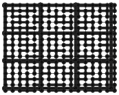
Figure 1. Subgraph reshaping algorithm applied on a graph representing an isotropic coefficient elliptic PDE.

Example 3.3.

Consider a graph Laplacian $\widehat{A}$ corresponding to a graph which is a $4\times 4$ square grid, on which all horizontal edges are weighted $1$ while all vertical edges are weighted $10$. Such graph Laplacian represents anisotropic coefficient elliptic equations with Neumann boundary conditions. Start with a non-optimal partitioning as shown on the left of Figure 2, of which the resulting two level method has a convergence rate $|E|_{\widehat{A}}=0.96$ and $|Q|_{\widehat{A}}^{2}=4.88$. After applying Algorithm 3, the refined aggregates have the shapes shown on the right of Figure 2, of which the two level convergence rate is reduced to $|E|_{\widehat{A}}=0.90$ and the energy of the coarse level projection is also reduced as $|Q|_{\widehat{A}}^{2}=1.50$.

$\qquad\longrightarrow\qquad$

Figure 2. Subgraph reshaping algorithm applied on a graph representing an anisotropic coefficient elliptic PDE.

4. Solve Phase

In this section, we discuss the parallelization of the solver phase on GPU. More precisely, we will focus on the parallel smoother, prolongation/restriction, MG cycle, and sparse matrix-vector multiplication.

4.1. Parallel Smoother

An efficient parallel smoother is crucial for the parallel AMG method. For the sequential AMG method, Gauss-Seidel relaxation is widely used and has been shown to have a good smoothing property. However the standard Gauss-Seidel is a sequential procedure that does not allow efficient parallel implementation. To improve the arithmetic intensity of the smoother and make it work better with SIMT based GPUs, we adopt the well-known Jacobi relaxation, and introducing a damping factor to improve the performance of the Jacobi smoother. For a matrix $A\in\mathbb{R}^{n\times n}$ and its diagonals are denoted by $D=\text{diag}(a_{11},a_{22},\cdots,a_{nn})$, the Jacobi smoother can be written in the following matrix form

$$x^{m+1}=x^{m}+\omega D^{-1}r^{m},\quad\text{where}\ r^{m}=b-Ax^{m},$$

or component-wise

$$x^{m+1}_{i}=x^{m}_{i}+\omega a_{ii}^{-1}r^{m}_{i}.$$

This procedure can be implemented efficiently on GPUs by assigning one thread to each component, and update the corresponding components locally and simultaneously.

We also consider the so-called $\ell^{1}$ Jacobi smoother, which is parameter free. Define

$$M=\text{diag}(M_{11},M_{22},\cdots,M_{nn}),$$

where $M_{ii}=a_{ii}+d_{ii}$ with $d_{ii}=\sum_{j\neq i}|a_{ij}|$, and the $\ell^{1}$ Jacobi has the following matrix form

$$x^{m+1}=x^{m}+M^{-1}r^{m},\quad\text{where}\ r^{m}=b-Ax^{m},$$

or component-wise

$$x^{m+1}_{i}=x^{m}_{i}+M_{ii}^{-1}r^{m}_{i}.$$

In [25, 7] it has been show that if $A$ is symmetric positive definite, the smoother is always convergent and has multigrid smoothing properties comparable to full Gauss-Seidel smoother if $a_{ii}\geq\theta d_{ii}$ and $\theta$ is bounded away from zero. Moreover, because its formula is very similar to the Jacobi smoother, it can also be implemented efficiently on GPUs by assigning one thread to each component, and update the corresponding the component locally and simultaneously.

4.2. Prolongation and Restriction

For UA-AMG method, the prolongation and restriction matrices are piecewise constant and characterize the aggregates. Therefore, we can preform the prolongation and restriction efficiently in UA-AMG method. Here, the output array aggregation (column index of $P$), which contains the information of aggregates, plays an important rule.

• Prolongation: Let $v^{l-1}\in\mathbb{R}^{n_{l-1}}$, so that the action $v^{l}=P_{l-1}^{l}v^{l-1}$ can be written component-wise as follows:

  $$(v^{l})_{i}=(P_{l-1}^{l}v^{l-1})_{i}=(v^{l-1})_{j},\quad j\in G^{l-1}_{i}$$

  Assign each thread to one element of $v^{l}$, and the array aggregation can be used to obtain information about $j\in G^{l-1}_{i}$, i.e., $i=\texttt{aggregation}[j]$, so that prolongation can be efficiently implemented in parallel.

• Restriction: Let $v^{l}\in\mathbb{R}^{n_{l}}$, so that the action $(P_{l-1}^{l})^{T}v^{l}$ can be written component-wise as follows:

  $$(v^{l-1})_{i}=((P_{l-1}^{l})^{T}v^{l})_{i}=\sum_{j\in G^{l-1}_{i}}(v^{l})_{j}.$$

  Therefore, each thread is assigned to an element of $v^{l-1}$, and the array aggregation can be used to obtain information about $j\in G^{j-1}_{i}$, i.e., to find all $j$ such that $\texttt{aggregation}[j]=i$. By doing so, the action of restriction can also be implemented in parallel.

4.3. K-cycle

Unfortunately, in general, UA-AMG with V-cycle is not an optimal algorithm in terms of convergence rate. But on the other hand, in many cases, UA-AMG using two-grid solver phase gives optimal convergence rate for graph Laplacian problems. This motivated us to use other cycles instead of V-cycle to mimic the two-grid algorithm. The idea is to invest more works on the coarse grid, and make the method become closer to an exact two-level method, then hopefully, the resulting cycle will have optimal convergence rate.

The particular cycle we will discuss here is the so-called K-cycle (Nonlinear AMLI-cycle) and we refer to [29, 1, 2] for details on its implementation in general.

4.4. Sparse Matrix-Vector Multiplication on GPUs

As the K-cycle will be used as a preconditioner for Nonlinear Preconditioned Conjugate Gradient (NPCG) method, the sparse matrix-vector multiplication (SpMV) has major contribution to the computational work involved. An efficient SpMV algorithm on GPU requires a suitable sparse matrix storage format. How different storage formats perform in SpMV is extensively studied in [4]. This study shows that the need for coalesce accessing of the memory makes ELLPACK (ELL) format one of the most efficient sparse matrix storage formats on GPUs when each row of the sparse matrix has roughly the same nonzeros. In our study, because our main focus is on the parallel aggregation algorithm and the performance of the UA-AMG method, we still use the compressed row storage (CSR) format, which has been widely used for the iterative linear solvers on CPU. Although this is not an ideal choice for GPU implementation, the numerical results in the next section already show the efficiency of our parallel AMG method.

5. Numerical Tests

In this section, we present numerical tests using the proposed parallel AMG methods. Whenever possible we compare the results with the CUSP libraries [15]. CUSP is an open source C++ library of generic parallel algorithms for sparse linear algebra and graph computations on CUDA-enabled GPUs. All CUSP’s algorithms and implementations have been optimized for GPU by NVIDIA’s research group. To the best of our knowledge, the parallel AMG method implemented in the CUSP package is the state-of-the-art AMG method on GPU. We use as test problems several discretizations of the Laplace equation.

5.1. Numerical Tests for Parallel Aggregation Algorithm

Define $Q$, the $\ell^{2}$ projection on the piece-wise constant space $\operatorname{Range}(P)$, as the following:

$$Q=P(P^{T}P)^{-1}P^{T}.$$

We present several tests showing how the energy norm of this projection changes with respect to different parameters used in the parallel aggregation algorithm, since the convergence rate is an increasing function of $\|Q\|_{A}$.

The tests involving $\|Q\|_{A}$ further suggest two additional features necessary to get a multigrid hierarchy with predictable results. First, the sizes of aggregates need to be limited, and second, the columns of the prolongator $P$ need to be ordered in a deterministic way, regardless of the order that aggregates are formed. The first requirement can be fulfilled simply by limiting the sizes of the aggregates in each pass of the parallel aggregation algorithm. We make the second requirement more specific. Let $c_{k}$ to be the index of the coarse vertex of the $k$-th aggregate. We require that $c_{k}$ should be an increasing sequence and then use the $k$-th column of $P$ to record the aggregate with the coarse vertex numbered $c_{k}$. This can be done by using a generalized version of the prefix sum algorithm [5].

We first show in Table 5.1 the coarsening ratios (in the parenthesis in the table) and the energy norms $\|Q\|_{A}^{2}$ of a two grid hierarchy, for a Laplace equation with Dirichlet boundary conditions on a structured grid containing $n^{2}$ vertices. The limit on the size of an aggregate is denoted by $t$, which suggests that, any aggregate can include $t$ vertices or less, which directly implies that the resulting coarsening ratio is less or equal to $t$.

	$t=2$	$t=3$	$t=4$	$t=5$
$n=128$	(1.99) 1.71	(2.03) 2.04	(2.41) 2.46	(2.97) 3.15
$n=256$	(1.99) 1.72	(2.39) 2.57	(2.96) 2.59	(2.99) 3.20
$n=512$	(2.00) 1.72	(2.01) 2.08	(2.40) 2.48	(2.99) 3.22

Table 5.1. (coarsening ratios) and energy norm of a two grid hierarchy of a Laplace equation on a uniform grid with Dirichlet boundary conditions.

For the same aggregations on the graphs that represent Laplace equations with Neumann boundary conditions, the corresponding coarsening ratio (in parenthesis) and $|Q|_{A}^{2}$ seminorms with respect to grid size $n$ and limiting threshold $t$ are shown in Table 5.2.

	$t=2$	$t=3$	$t=4$	$t=5$
$n=128$	(1.99) 1.87	(2.03) 2.11	(2.41) 2.48	(2.97) 3.24
$n=256$	(1.99) 1.74	(2.39) 2.59	(2.96) 2.62	(2.99) 3.24
$n=512$	(2.00) 1.87	(2.01) 2.11	(2.40) 2.49	(2.99) 3.24

Table 5.2. (coarsening ratios) and energy norm of a two grid hierarchy of a Laplace equation on a uniform grid with Neumann boundary conditions.

In Table 5.3 we present the computed bounds on the coarsening ratio and energy of a two level hierarchyBy energy of a two level hierarchy here, we mean the semi-norm of the $\ell^{2}$ projection on the coarse space. when the fine level is an $n\times n$. Such results are valid for any structured grid with $n^{2}$ vertices (not just $n=126,\ldots,132$) This is seen as follows: (1) From equation (3.2), it follows that if we consider two grids of sizes $n_{1}\times n_{1}$ and $n_{2}\times n_{2}$ respectively, and such that

$$(n_{1}-n_{2})\equiv 0\mod 12,\quad\text{ or }\quad(n_{1}+n_{2})\equiv 0\mod 12$$

then our aggregation algorithm results in the same pattern of $C$ points on these two grids; (2) As a consequence grids of size $n\times n$ for $n=126\equiv 6\mod 12$ to $n=132\equiv 0\mod 12$ give all possible coarsening patterns that can be obtained by our aggregation algorithm on any 2D tensor product grid. As a conclusion, the values of the coarsening ratios and the energy semi-norm given in Table 5.3 are valid for any 2D structured grid.

	$t=2$	$t=3$	$t=4$	$t=5$
$n=126$	(2.00) 2.11	(2.00) 2.07	(2.36) 2.73	(2.36) 2.73
$n=127$	(1.99) 1.86	(2.01) 1.98	(2.01) 2.49	(2.01) 2.34
$n=128$	(1.99) 1.71	(2.03) 2.04	(2.41) 2.47	(2.97) 3.15
$n=129$	(1.99) 1.84	(2.02) 2.04	(2.03) 2.31	(2.02) 2.42
$n=130$	(1.99) 1.77	(2.40) 2.21	(2.92) 2.86	(2.94) 2.94
$n=131$	(1.99) 2.61	(2.01) 2.41	(2.01) 2.45	(2.00) 2.49
$n=132$	(1.98) 2.09	(2.21) 2.81	(2.33) 2.89	(2.26) 2.94

Table 5.3. (coarsening ratios) and energy norm of a two grid hierarchy of a Laplace equation on a uniform grid with Neumann boundary conditions.

We also apply this aggregation method on graphs corresponding to Laplace equations on 2 dimensional unstructured grids with Dirichlet or Neumann boundary conditions. The unstructured grids are constructed by perturbing nodes in an $n\times n$ square lattice ($n=128,256,512$), followed by triangulating the set of perturbed points using a Delaunay triangulation. The condition numbers of the Laplacians, derived using finite element discretization of the Laplace equations on the mentioned unstructured grids with Dirichlet boundary conditions, are about $1.2\times 10^{4}$, $5.0\times 10^{4}$, and $2.1\times 10^{5}$ respectively. The coarsening ratios and $|Q|_{A}^{2}$ are listed in table 5.4 and 5.5. We remark here that we also apply the parallel aggregation algorithm without imposing limit on the size of an aggregate, and the corresponding numerical results are listed in columns named “$t=\infty$”.

	$t=2$	$t=3$	$t=4$	$t=5$	$t=\infty$
$n=128$	(1.80) 2.39	(2.53) 2.44	(3.17) 3.10	(3.73) 3.46	(4.91) 3.30
$n=256$	(1.79) 2.39	(2.52) 2.60	(3.15) 3.18	(3.69) 3.46	(4.91) 3.41
$n=512$	(1.80) 2.38	(2.55) 2.67	(3.19) 3.26	(3.72) 3.56	(4.93) 3.40

Table 5.4. (coarsening ratios) and energy norm of a two grid hierarchy of a Laplace equation with Dirichlet boundary conditions discretized on an unstructured grid.

	$t=2$	$t=3$	$t=4$	$t=5$	$t=\infty$
$n=128$	(1.80) 2.39	(2.53) 2.54	(3.17) 3.18	(3.73) 3.48	(4.91) 3.33
$n=256$	(1.79) 2.49	(2.52) 2.65	(3.15) 3.20	(3.69) 3.48	(4.91) 3.41
$n=512$	(1.80) 2.47	(2.55) 2.80	(3.19) 3.27	(3.72) 3.57	(4.93) 3.53

Table 5.5. (coarsening ratios) and energy norm of a two grid hierarchy of a Laplace equation with Neumann boundary conditions discretized on an unstructured grid.

We note that in Table 5.4 and Table 5.5, the coarsening ratios are not large enough to result in small operator complexity. We then estimate the energy norm $|Q|_{A}^{2}$ when $Q$ is the $\ell^{2}$ orthogonal projection from any level of the multigrid hierarchy to any succeeding sub-levels. We start with a Laplace equation on a $128^{2}$ structured square grid, set the limit of sizes of aggregates as $t=5$ on each iteration of aggregation, and stop when the coarsest level is of less than 100 degrees of freedom. If denoting the finest level by level 0, and the coarsest level we get is level 5. The coarsening ratios and energy norm $|Q|_{A}^{2}$ between any two levels are shown in table 5.6 and 5.7.

	0	1	2	3	4
1	(2.97) 3.15	-	-	-	-
2	(11.3) 7.34	(3.81) 3.09	-	-	-
3	(38.6) 15.3	(13.0) 6.74	(3.41) 2.68	-	-
4	(113.8) 31.9	(38.3) 13.9	(10.1) 5.25	(2.95) 3.91	-
5	(321.3) 54.5	(108.2) 22.5	(28.4) 9.09	(8.33) 4.53	(2.82) 4.77

Table 5.6. (coarsening ratios) and energy norms squares of a multigrid hierarchy of a Laplace equation with Dirichlet boundary conditions discretized on a $128^{2}$ grid.

	0	1	2	3	4
1	(2.97) 3.23	-	-	-	-
2	(11.3) 7.68	(3.81) 3.28	-	-	-
3	(38.6) 16.9	(13.0) 7.99	(3.41) 2.94	-	-
4	(113.8) 42.5	(38.3) 20.6	(10.1) 7.07	(2.95) 4.23	-
5	(321.3) 98.6	(108.2) 48.3	(28.4) 17.0	(8.33) 7.11	(2.82) 5.75

Table 5.7. (coarsening ratios) and energy norm of a multigrid hierarchy of a Laplace equation with Neumann boundary conditions discretized on a $128^{2}$ grid.

We observe that, on the diagonal of the table 5.6 and 5.7, the energy norms are comparable to the coarsening ratios, until the last level where the grid becomes highly unstructured. This suggests that a linear or nonlinear AMLI solving cycle can give both a good convergence rate and a favorable complexity. It is also observed that, on the lower triangular part of the table 5.6-5.7, the energy norms are always smaller than the corresponding coarsening ratios, which motives us to design in the future flexible cycles that detect and skip unnecessary levels.

Another inspiring observation is that, in Table 5.1, even if we set a limit $t=5$ for the maximal number of vertices in an aggregate, the resulting aggregates have an average number of vertices ranging from $2.97$ to $2.99$. We plot the aggregates of an unweighted graph corresponding to a $16\times 16$ square grid on the left of Figure 3, and observe that, some aggregates contain 5 vertices and some contains only 1. We then use the rank one optimization discussed in Section 3.3 and apply subgraph reshaping algorithm (Algorithm 3) as a post-process of the GPU parallel aggregation algorithm (Algorithm 2), and plot the resulting aggregates on the right of Figure 3. Since the subgraph reshaping algorithm does not change the number of aggregates, the coarsening ratios on the left and right of Figure 3 are identical and are equal to $2.72$. The energy of the $\ell^{2}$ projection is deceased from $|Q|_{\widehat{A}}^{2}=2.51$ (left of Figure 3) to $|Q|_{\widehat{A}}^{2}=2.19$ (right of Figure 3). However, two level convergence rate increases from $|E|_{\widehat{A}}=0.67$ (left of Figure 3) to $|E|_{\widehat{A}}=0.69$ (right of Figure 3).

$\longrightarrow$

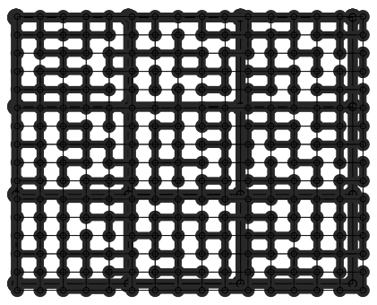
Figure 3. Before (left) and after (right) the Subgraph Reshaping Algorithm applied on partitioning given by Parallel Aggregation Algorithm.

Some more comments on the reshaping algorithm are in order. For isotropic problems, the reshaping does not have significant impact of on the convergence rate because aggregation obtained by standard approach already results in a good convergence rate. However, for anisotropic problems reshaping improves the convergence rate. In this case, starting with aggregates of arbitrary shape, the reshaping procedure results in aggregates aligned with the anisotropy and definitely improves the overall convergence rate.

In addition, even for isotropic case, the numerical results in the manuscript indicate that subgraph reshaping can be essential for variety of cycling algorithms when aggressive coarsening is applied. As shown in Example 3.2 and Example 3.3, the aggregation reshaping helps for some isotropic and anisotropic problems when coarsening ratio is 8. In Table 5.6 and Table 5.7, we observe that such coarsening ratio can be achieved by skipping every other level in our current multilevel hierarchy.

Clearly, further investigation about the reshaping is needed for more general problems that have both anisotropic and isotropic regions. Analyzing such cases as well as testing how much improvement in the convergence can be achieved by subgraph reshaping for specific coarsening and cycling strategies are subject of an ongoing and future research.

5.2. Numerical Tests for GPU Implementation

In this section, we perform numerical experiments to demonstrate the efficiency of our proposed AMG method and discuss the specifics related to the use of GPUs as main platform for computations. We test the parallel algorithm on Laplace equation discretized on quasi-uniform grids in 2D. Our test and comparison platform is the NVIDIA Tesla C2070 together with a Dell computing workstation. Details in regard to the machine are given in Table 5.8.

CPU Type	Intel
CPU Clock	2.4 GHz
Host Memory	16 GB
GPU Type	NVIDIA Tesla C2070
GPU Clock	575MHz
Device Memory	6 GB
CUDA Capability	2.0
Operating System	RedHat
CUDA Driver	CUDA 4.1
Host Complier	gcc 4.1
Device Complier	nvcc 4.1
CUSP	v0.3.0

Table 5.8. Test Platform

Because our aim is to demonstrate the improvement of our algorithm on GPUs, we concentrate on comparing the method we describe here with the parallel smoothed aggregation AMG method implemented in the CUSP package [15].

We consider the standard linear finite element method for the Laplace equation on unstructured meshes. The results are shown in the Table 5.9. Here, CUSP uses smoothed aggregation AMG method with V-cycles, and our method is UA-AMG with K-cycles. The stoping criterion is that the $\ell^{2}$ norm of the relative residual is less than $10^{-6}$. According to the results, we can see that our parallel UA-AMG method converges uniformly with respect to the problem size. This is due the improved aggregation algorithm constructed by our parallel aggregation method and the K-cycle used in the solver phase. We can see that our method is about 3 to 4 times faster in setup phase, which demonstrate the efficiency of our parallel aggregation algorithm. In the solver phase, due to the factor that we use K-cycle, which does much more work on the coarse grids, our solver phase is a little bit slower than the solver phase implemented in CUSP. However, the use of a K-cycle yields a uniformly convergent UA-AMG method, which is an essential property for designing scalable solvers. When the size of the problem gets larger, we expect the computational time of our AMG method to scale linearly whereas the AMG method in CUSP seems to grows faster than linear and will be slower than our solver phase eventually. Overall, our new AMG solver is about $1.5$ times faster than the smoothed aggregation AMG method in CUSP in terms of total computational time, and the numerical tests suggests that it converges uniformly for the Poisson problem.

	#DoF = 1 million				#DoF = 4 million
	# Iter.	Setup	Solve	Total	# Iter.	Setup	Solve	Total
CUSP	36	0.63	0.35	0.98	41	2.38	1.60	3.98
New	19	0.13	0.47	0.60	19	0.62	2.01	2.63

Table 5.9. Comparison between the parallel AMG method in CUSP package (smoothed aggregation AMG with V-cycles) and our new parallel AMG method (UA-AMG with K-cycles).

References

- [1] O. Axelsson and P. S. Vassilevski. Algebraic multilevel preconditioning methods. I. Numer. Math., 56(2-3):157–177, 1989.
- [2] O. Axelsson and P. S. Vassilevski. Algebraic multilevel preconditioning methods. II. SIAM J. Numer. Anal., 27(6):1569–1590, 1990.
- [3] N. Bell, S. Dalton, and L. Olson. Exposing fine-grained parallelism in algebraic multigrid methods. SIAM Journal on Scientific Computing, 34(4):C123–C152, 2012.
- [4] N. Bell and M. Garland. Efficient sparse matrix-vector multiplication on CUDA. Technical Report NVR-2008-004, NVIDIA Corporation, 2008.
- [5] G. E. Blelloch. Prefix sums and their applications. In Synthesis of Parallel Algorithms. Morgan Kaufmann, 1993.
- [6] J. Bolz, I. Farmer, E. Grinspun, and P. Schröder. Sparse matrix solvers on the gpu: conjugate gradients and multigrid. ACM Trans. Graph., 22(3):917–924, 2003.
- [7] M. Brezina and P. S. Vassilevski. Smoothed aggregation spectral element agglomeration AMG: SA-AMGe. In Proceedings of the 8th international conference on Large-Scale Scientific Computing, volume 7116 of Lecture Notes in Computer Science, pages 3–15. Springer-Verlag, 2012.
- [8] E. Chow, R. Falgout, J. Hu, R. Tuminaro, and U. Yang. A survey of parallelization techniques for multigrid solvers. In Parallel processing for scientific computing, volume 20, pages 179–201. SIAM, 2006.
- [9] A. J. Cleary, R. D. Falgout, V. E. Henson, and J. E. Jones. Coarse-grid selection for parallel algebraic multigrid. In Solving Irregularly Structured Problems in Parallel, volume 1457 of Lecture Notes in Computer Science, pages 104–115. Springer, 1998.
- [10] R. Courant and D. Hilbert. Methods of mathematical physics. Vol. I. Wiley Classics Library. John Wiley & Sons Inc., 1989.
- [11] H. De Sterck, U. M. Yang, and J. J. Heys. Reducing complexity in parallel algebraic multigrid preconditioners. SIAM. J. Matrix Anal. & Appl., 27(4):1019–1039, 2006.
- [12] M. Emans, M. Liebmann, and B. Basara. Steps towards GPU accelerated aggregation AMG. In 2012 11th International Symposium on Parallel and Distributed Computing (ISPDC), pages 79–86, 2012.
- [13] C. Feng, S. Shu, J. Xu, and C.-S. Zhang. Numerical Study of Geometric Multigrid Methods on CPU–GPU Heterogeneous Computers. ArXiv e-prints, Aug. 2012.
- [14] Z. Feng and Z. Zeng. Parallel multigrid preconditioning on graphics processing units (gpus) for robust power grid analysis. In Proceedings of the 47th Design Automation Conference, DAC ’10, pages 661–666. ACM, 2010.
- [15] M. Garland and N. Bell. CUSP: Generic parallel algorithms for sparse matrix and graph computations, 2010.
- [16] D. Goddeke, R. Strzodka, J. Mohd-Yusof, P. McCormick, H. Wobker, C. Becker, and S. Turek. Using GPUs to improve multigrid solver performance on a cluster. International Journal of Computational Science and Engineering, 4(1):36–55, 2008.
- [17] N. Goodnight, C. Woolley, G. Lewin, D. Luebke, and G. Humphreys. A multigrid solver for boundary value problems using programmable graphics hardware. ACM SIGGRAPH 2005 Courses on SIGGRAPH 05, 2003(2003):193, 2003.
- [18] H. Grossauer and P. Thoman. GPU-based multigrid: Real-time performance in high resolution nonlinear image processing. International Journal of Computer Vision, pages 141–150, 2008.
- [19] G. Haase, M. Liebmann, C. Douglas, and G. Plank. A parallel algebraic multigrid solver on graphics processing units. In High Performance Computing and Applications, pages 38–47, 2010.
- [20] P. R. Halmos. Finite-dimensional vector spaces. Springer-Verlag, New York, second edition, 1974. Undergraduate Texts in Mathematics.
- [21] V. E. Henson and U. M. Yang. BoomerAMG: A parallel algebraic multigrid solver and preconditioner. Applied Numerical Mathematics, 41(1):155–177, 2002.
- [22] W. Joubert and J. Cullum. Scalable algebraic multigrid on 3500 processors. Electronic Transactions on Numerical Analysis, 23:105–128, 2006.
- [23] G. Karypis and V. Kumar. A parallel algorithm for multilevel graph partitioning and sparse matrix ordering. Journal of Parallel and Distributed Computing, 48:71–85, 1998.
- [24] G. Karypis and V. Kumar. Parallel multilevel k-way partitioning scheme for irregular graphs. SIAM Review, 41(2):278–300, 1999.
- [25] T. V. Kolev and P. S. Vassilevski. Parallel auxiliary space AMG for problems. J. Comput. Math., 27(5):604–623, 2009.
- [26] J. Kraus and M. Förster. Efficient AMG on heterogeneous systems. In Facing the Multicore - Challenge II, volume 7174 of Lecture Notes in Computer Science, pages 133–146. Springer Berlin Heidelberg, 2012.
- [27] A. Krechel and K. Stüben. Parallel algebraic multigrid based on subdomain blocking. Parallel Computing, 27(8):1009–1031, 2001.
- [28] R. S. Tuminaro. Parallel smoothed aggregation multigrid: aggregation strategies on massively parallel machines. In Proceedings of the 2000 ACM/IEEE conference on Supercomputing (CDROM). IEEE, 2000.
- [29] P. S. Vassilevski. Multilevel block factorization preconditioners. Springer, New York, 2008.