Effects of electron scattering on the topological properties of nanowires: Majorana fermions from disorder and superlattices

Abstract

We focus on inducing topological state from regular, or irregular scattering in (i) p-wave superconducting wires and (ii) Rashba wires proximity coupled to an s-wave superconductor. We find that contrary to common expectations the topological properties of both systems are fundamentally different: In p-wave wires, disorder generally has a detrimental effect on the topological order and the topological state is destroyed beyond a critical disorder strength. In contrast, in Rashba wires, which are relevant for recent experiments, disorder can induce topological order, reducing the need for quasiballistic samples to obtain Majorana fermions. Moreover, we find that the total phase space area of the topological state is conserved for long disordered Rashba wires, and can even be increased in an appropriately engineered superlattice potential.

I Introduction

The response of conventional s-wave superconductors to nonmagnetic disorder is drastically different from that of nonconventional superconductors with higher angular momentum pairing. While s-wave superconductivity is resistant to the presence of nonmagnetic disorder, it is detrimental to unconventional superconductivity Anderson59 ; Abrikosov60 . Other than the pairing symmetry, superconductors are also classified by the structure of their quasiparticle excitations: those that can be adiabatically transformed into a conventional insulator are topologically trivial. The topologically nontrivial superconductors on the other hand are distinguished by exotic low-energy excitations at their boundaries. In one dimension, these excitations turn out to be their own antiparticles and are dubbed Majorana fermions. Thus, Majorana fermions can appear at the ends of a spinless p-wave superconducting wire Kitaev01 or at the ends of a spin-orbit coupled semiconductor quantum wire in proximity to a conventional s-wave superconductor Lutchyn10 ; Oreg10 .

The latter, hybrid system reduces to an effective p-wave superconductor Alicea11 in the limit of an almost depleted wire. For this reason, the topological properties of p-wave superconducting wires and hybrid nanowire systems with s-wave superconductivity are commonly assumed to be equivalent Alicea12 ; Leijnse12 . In particular, the effects of disorder on the topological superconductivity (and thus on the Majorana fermion) have so far been explored mainly within this premise. The main conclusion of these works is that disorder is always detrimental to the topological superconductivity and hence the Majorana fermion can survive only if (i) the mobility is high enough such that the localization length is longer than the coherence length of the topological superconductor Piet11 ; Piet11a ; Potter11 ; Sau12 ; Maresa12 and (ii) there is an odd number of spin-resolved transverse modes in a multi-mode wire Wimmer10 ; Potter10 ; Stanescu11 ; Piet12 .

The recent observation of a zero-bias peak (ZBP) in the Andreev conductance of superconducting InSb nanowire heterostructures mourik12 , followed by similar observations subsequentially reported by other groups Deng12 ; Das12 , therefore raised many questions about the origin of the peak because the mean free path obtained from normal state conductance shows the nanowires to be too dirty to be in the topological regime. Indeed, recent works caution against the interpretation that these peaks are signatures of Majorana fermions Liu12 ; Bagrets12 ; Pikulin12 ; Rainis13 .

In contrast, here we show that topological superconductivity in the presence of s-wave order parameter is resistant to disorder in that the conditions (i) and (ii) are in fact not essential for the survival of Majorana fermions. The underlying reason (which is not captured by an effective p-wave model) is that a transport gap can be utilized to induce and protect topological state similar to the spectral gaps of conventional proposals. Hence, disorder can induce robust topological order in s-wave superconductors and thus create Majorana fermions. Indeed, we find that, for long disordered wires, the total area of the topological phase is conserved. Strikingly, if the scattering is regular e.g. due to a superlattice, the area of the topological phase can be made to increase beyond the clean value, raising the possibility to further engineer topological order.

This article is organized as follows: we develop a theory capable of studying topological phase transitions in the presence of individual (possibly random) potential configurations, rather than calculating average quantities. First, we focus on the almost depleted wire and recover in the weak-disorder limit the earlier results of Refs. Motrunich01 ; Piet11 , namely that disorder is always detrimental to the topological order for p-wave superconductors. We then show how, for individual disorder configurations, one can relate the phase diagram to an experimentally accessible quantity: the normal state conductance. This result allows us to solve inter alia the Gaussian disordered p-wave problem exactly for all values of the disorder strength (Fig. 1). Finally, we focus on the experimentally relevant case of a semiconductor nanowire with s-wave superconductivity. We find that, unlike its p-wave counterpart, topological s-wave superconductivity is resistant to disorder (Fig. 2).

II Spinless p-wave superconducting wire

We start with the spinless p-wave Hamiltonian, as the calculation is easier to follow and illustrates the essential concepts. We note that the disordered p-wave model was solved at half-filling as well as for specific position-dependent potentials Lang12 ; DeGottardi12 . Here, we present a general solution.

The Bogoliubov-de Gennes (BdG) Hamiltonian for a spinless $p$-wave superconductor in one dimension is:

$$H=h(p,x)\tau_{z}+u\,p\,\tau_{x},$$ (1)

where $h(p,x)=p^{2}/2m+V(x)-\mu$ is the (spinless) single-particle Hamiltonian, $p$ is the momentum operator, $m$ the electron mass, $V(x)$ the single-particle potential, $\mu$ the chemical potential, and $u\,p$ the p-wave pairing operator. Here and below $\tau_{i}$ ($i=x,y,z$) denote the Pauli matrices in the electron-hole space. In order to make use of the chiral symmetry of the Hamiltonian, we apply a unitary transformation with $U=\exp(i\tau_{x}\pi/4)$, that casts the Hamiltonian into an off-diagonal form. We note that similar argumentation was used to study zero modes in d-wave superconductors inanc99 . The energy $E=0$ Majorana fermion solutions are then either of the form $\chi_{+}=\bigl{(}{\varphi_{+}\atop{0}}\bigr{)}$ or of the form $\chi_{-}=\bigl{(}{0\atop{\varphi_{-}}}\bigr{)}$, with $\varphi_{\pm}={\rm e}^{\pm k_{u}x}\psi$, where $k_{u}=mu/\hbar$ and $\psi$ locally satisfies the normal state equation $h(p,x)\psi=-(\hbar^{2}k_{u}^{2}/2m)\psi$. However, it is $\varphi_{\pm}$ that needs to be normalized, rather than $\psi$ itself. Hence a diverging solution $\psi$ as $x\rightarrow\pm\infty$ is permissible if the divergence is not faster than ${\rm e}^{\pm k_{u}x}$.

We now construct the Majorana fermion state. For the sake of concreteness, we consider an interface between an half infinite ($x>0$) wire, with the vacuum $x<0$ (a normal insulator) implemented via the boundary condition (BC) $\chi(0)=0$. We note that, it is easy to generalize to BCs of the form $a\chi(x_{0})+b\frac{d\chi}{dx}|_{x_{0}}=0$. We also require $\chi\rightarrow 0$ sufficiently fast as $x\rightarrow\infty$ to ensure normalizability. Then, choosing $\psi=g(0)f(x)-f(0)g(x)$, with $f$ and $g$ the local solutions of the normal state equation, ensures that $\chi$ fulfills the BC at $x=0$. We focus on solutions that behave as $\psi\sim e^{\Lambda x}a(x)$ for large $x$, with $a(x)$ a nondivergent function and $\Lambda(\bar{\mu})$ a real function of $\bar{\mu}=\mu-\hbar^{2}k_{u}^{2}/2m$. For solutions that diverge or decay faster (slower) than $e^{\Lambda x}$ we set $\Lambda={\rm sgn}(\Lambda)\times\infty$ ($\Lambda=0$). We identify three cases (i) $\Lambda<-k_{u}$, (ii) $|\Lambda|<k_{u}$, and (iii) $k_{u}<\Lambda$. For case (i) $\psi$ is a bound normal state solution that fulfills both BCs and there are two zero modes $\chi_{+}$ and $\chi_{-}$. Under a small perturbation, $\psi$ no longer satisfies the BCs, and hence the two solutions $\chi_{\pm}$ will shift away from $E=0$, i.e. they are not topologically protected. This corresponds to an accidental level crossing at $E=0$ footnote_accidental . In case (ii) there is only one state, $\chi_{-}$, the topologically protected Majorana state, and in case (iii) there are no zero modes and thus no Majorana state. We thus obtain a formula for the topological charge:

$${\cal Q}={\rm sgn}\left(\left|\Lambda(\mu-\hbar^{2}k_{u}^{2}/2m)\right|/k_{u}-1\right),$$ (2)

where ${\cal Q}=-1$ means the wire is topological. This is the central result for the $p-$wave part of our work.

The topological robustness of the zero energy solutions is due to the fact that only the asymptotic limit of the solution $\psi$ of the effective Schrödinger equation matters for its existence. Any local perturbation (unless infinite) cannot change this asymptotic limit.

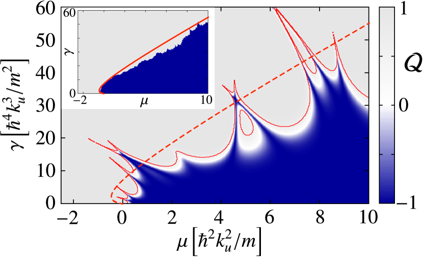
Figure 1: Topological charge of a disordered p-wave wire as a function of $\mu$ and disorder strength $\gamma$, for a single disorder configuration in a short wire ($L=100a$, with $a$ the lattice constant). The inset shows a single disorder configuration in a long wire ($L=10000a$). The red solid line is the phase boundary computed from Eqs. (2) and the normal state conductance $G$, the red dashed lines are from Eqs. (2) and (3). The numerical calculation was done in a TB model with $k_{u}=10a^{-1}$ and a chemical potential in the leads $\mu_{\text{lead}}=0.5\hbar^{2}/2ma^{2}$.

For a disordered (normal-state) wire, $\Lambda$ is called the Lyapunov exponent and can be estimated from the conductance as: $\Lambda=-\log(G/G_{0})/2L,$ where $L$ is the wire length and $G_{0}$ the conductance quantum RMT_Carlo . Hence, for fixed $u$, Eq. (2) determines the topological charge of a p-wave quantum wire from its normal state conductance alone. In short wires, $\Lambda$ fluctuates strongly as the chemical potential varies, leading to multiple changes of the topological phase. This is shown on the example of a single disorder realization in a short wire in Fig. 1, where we computed the topological charge within a tight-binding (TB) model from $Q=\det(r)$ where $r$ is the reflection matrix Akhmerov11 . The numerical computation was performed using the Kwant code Kwant . The topological phase boundary computed from Eq. (2) and the numerically computed normal state conductance agrees very well with the $\det(r)$-criterion; small deviations of the exact position of the phase boundary are due to finite size effects.

For longer wires the Lyapunov exponent is a self averaging quantity, i.e. $\Lambda(L)\rightarrow\bar{\Lambda}$, as $L\rightarrow\infty$, where $\bar{\Lambda}$ is the average Lyapunov exponent RMT_Carlo . For a wire with Gaussian disorder $\langle V(x)V(y)\rangle=\gamma\delta(x-y)$ at energy $\epsilon$, it can be obtained in closed form Halperin65 ; ItzDrou :

$$\!\!\!\!\bar{\Lambda}(\epsilon)\!\! = \!\!\frac{m^{1/2}}{\hbar\lambda}F\big{(}\lambda^{2}\epsilon\big{)},\quad\leavevmode\nobreak\ \leavevmode\nobreak\ \lambda=\left(\frac{\hbar}{\gamma m^{1/2}}\right)^{1/3},$$ (3a)

$$\!\!\!\!F(x)\!\! = \!\!-\frac{1}{2}\frac{d\ln\Big{(}{\rm Ai}\big{(}\!-\!2^{1/3}x\big{)}^{2}+{\rm Bi}\big{(}\!-\!2^{1/3}x\big{)}^{2}\Big{)}}{dx}.$$ (3b)

Then the topological transition condition Eq. (2) becomes $\hbar|\bar{\Lambda}(\mu-mu^{2}/2)|=mu$, valid for the entire range of $\mu$, $u$, $\gamma$ and shown as a red dashed line in Fig. 1 and its inset. The inset also shows numerics for a single disorder configuration for a long wire, demonstrating that due to the self-averaging long wires have a well-defined universal topological phase (similar numerics, as well as an argument for weak disorder was presented in Pientka12 ). At high energies, we have the golden rule result $\Lambda\sim 1/4\ell_{\text{tr}}$, where $\ell_{\text{tr}}=\hbar^{2}(\mu-mu^{2}/2)/\gamma m$ is the transport mean free path, and find a topological transition at $k_{u}\ell_{\text{tr}}=1/4$, in agreement with Ref. Piet11 ; footnotefactor2 .

From Eq. (2) it can be also concluded that for $\bar{\mu}>0$ any scattering is detrimental to the topological phase: Then $\Lambda=0$ in the clean system and any scattering leads to $\Lambda\geq 0$. For $\bar{\mu}<0$, potential fluctuations generate islands of topological regions which may hybridize to induce a topological state as seen in the inset of Fig. 1. However, this is a relatively small effect. We shall see below this picture is drastically different for the experimentally relevant proximity nanowire systems.

III Rashba wire in proximity to an s-wave superconductor

We now focus on the experimentally more relevant system: a nanowire with Rashba spin-orbit coupling (SOC) in proximity to an s-wave superconductor. The BdG Hamiltonian is then given as Lutchyn10 ; Oreg10 :

$$H=h(p,x)\tau_{z}+\alpha p\sigma_{y}\tau_{z}+B\sigma_{x}+\Delta\tau_{x},$$ (4)

where $h(p,x)=p^{2}/2m+V(x)-\mu$ is the (spinless) single-particle Hamiltonian, $\alpha$ the SOC strength, $B$ the Zeeman splitting and $\Delta$ the induced s-wave order parameter. $\sigma_{i}$ ($i=x,y,z$) are the Pauli matrices in spin space. The topological state appears for $B^{2}>\Delta^{2}+\mu^{2}$. In this single orbital mode limit, the system is in class BDI, which is distinguished from class D by the presence of the chiral symmetry. This allows to bring the Hamiltonian into off-diagonal form Tewari12 , and a solution can be found in a similar spirit to the p-wave case considered above (details of the calculation can be found in the Appendix). In particular, the zero-energy Majorana states are of again of the form $\chi_{+}=\bigl{(}{\phi_{+}\atop{0}}\bigr{)}$ or $\chi_{-}=\bigl{(}{0\atop{\phi_{-}}}\bigr{)}$, but it the present case $\phi_{\pm}$ is a spinor satisfying a $2\times 2$ nonhermitian eigenvalue problem:

$$(h(p,x)\sigma_{z}\pm B\pm\Delta\sigma_{x}-i\alpha p\sigma_{x})\phi_{\pm}=0$$ (5)

Zero-energy solutions of this equations can be found in closed form only for small $\alpha$, but larger values of SOC do not change the qualitative picture, but rather renormalize the topological-normal phase boundaries. To order $\alpha^{2}$ the solution reads

$$\phi_{\pm}=\xi_{\pm}(\epsilon){\rm e}^{\pm\kappa x}\big{(}Af(x;\epsilon)+Bg(x;\epsilon)\big{)}$$

$$\quad\quad+\xi_{\pm}(-\epsilon){\rm e}^{\mp\kappa x}\big{(}Cf(x;-\epsilon)+Dg(x;-\epsilon)\big{)},$$ (6)

where $\epsilon=\sqrt{B^{2}-\Delta^{2}}$, $\kappa=m\alpha\Delta/\hbar\epsilon$, and $\xi_{+}(\epsilon)$ is the eigenvectors of the $2\times 2$ matrix $\epsilon\sigma_{z}+\Delta\sigma_{x}$ with positive eigenvalue. $f(x;\epsilon)$ and $g(x;\epsilon)$ are, as above, the two linearly independent solutions of $h(p,x)\psi=\epsilon\psi$, with $f$ decaying and $g$ increasing. Then, $\phi_{\pm}$ is a zero-energy Majorana state if it is normalizable and satisfies the BCs.

We assume again without loss of generality that the system is in a normal insulator state for $x<0$ and the BC $\phi(0)=0$. We identify three cases: (i) If $B>\Delta$, and $|\Lambda(\mu\pm\epsilon)|<|\kappa|$ or $|\Lambda(\mu\pm\epsilon)|>|\kappa|$, there are two decaying and two diverging solutions and the BC at $x=0$ can only be satisfied accidentally, namely if $f(0,\pm\epsilon)=0$. Then there is also a second solution in the other sector, and the zero-energy states are not protected. The system is thus in the trivial state with the possibility of accidental zero modes. (ii) If $B<\Delta$, then both $\kappa$ and $\epsilon$ are imaginary, hence there are always two decaying and two diverging solutions. However, there are no accidental zero modes with $f(\pm\epsilon)$ already fulfilling the BC because this would mean $f$ is an eigenfunction of (Hermitian) $h$ with an imaginary eigenvalue. (iii) If $B>\Delta$ and $|\Lambda(\mu\pm\epsilon)|<|\kappa|<|\Lambda(\mu\mp\epsilon)|$, there are one diverging and three decaying solutions in one sector and one decaying and three diverging solutions in the other sector. Then the BC at $x=0$ can be generally satisfied in the sector that has three decaying solutions and there is a Majorana state. As before, the solution is robust, because local perturbations do not change the asymptotic behavior of $f$ and $g$. In summary we have:

$${\cal Q}={\rm sgn}\left(\frac{|\Lambda(\mu+\epsilon)|}{m\alpha\Delta/\hbar\epsilon}-1\right)\,{\rm sgn}\left(\frac{|\Lambda(\mu-\epsilon)|}{m\alpha\Delta/\hbar\epsilon}-1\right).$$ (7)

This is our central formula for the s-wave case. The first term in Eq. (7) reduces to Eq. (2) in the large $B$-limit (i.e. only the “spin-down” band is contributing), recovering the p-wave result, while the second term is due to the presence of the “spin-up” band and introduces new physics. In summary, a transport gap in one of the “spin-bands” induces topology in the other “spin-band”, in contrast to the clean case where one spin-band is removed by a spectral (Zeeman) gap.

We now apply our formula Eq. (7) to the case of regular scattering (i.e. from a superlattice). For a clean wire, the required odd number of channels for the topological state is only achieved if the chemical potential is within the Zeeman gap Lutchyn10 ; Oreg10 . The perfect backscattering from a superlattice (or equivalently, minigaps) allow this for a larger range of $\mu$. Strikingly, even a superlattice formed from topologically trivial pieces can be topological. In summary, regular scattering can induce topological order out of the Zeeman gap, enlarging the topological phase area beyond its clean wire value, as shown in Fig. 2(a,b).

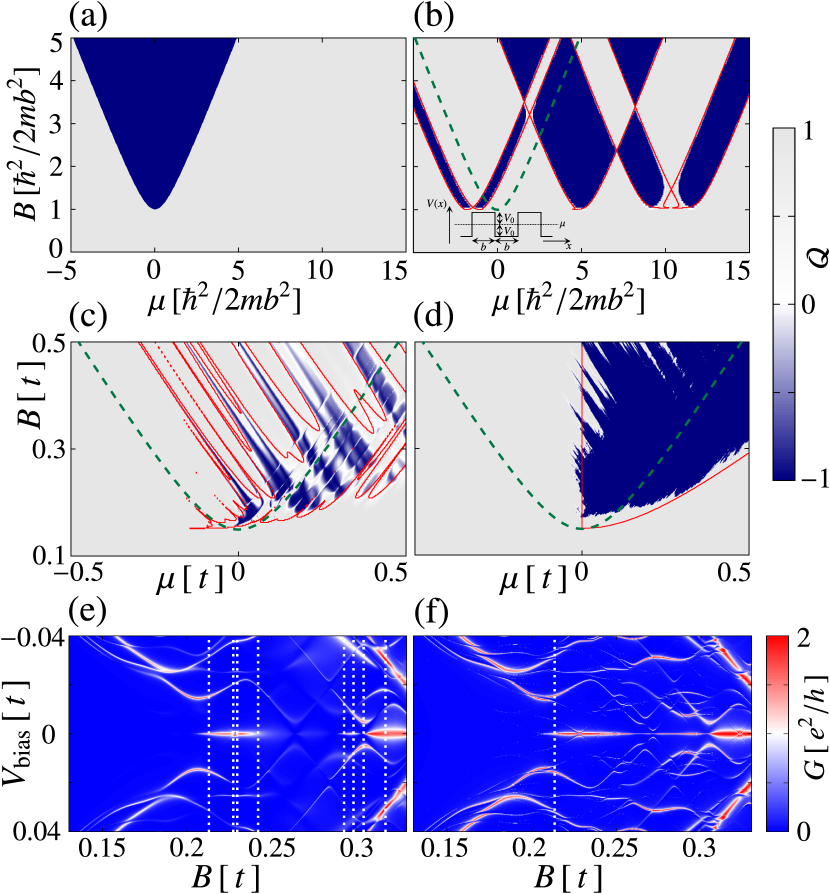
Figure 2: Topological charge as a function of chemical potential $\mu$ and Zeeman splitting $B$ for a (a) clean system, (b) a superlattice, and (c, d) disorder. Red lines in (b-d) are phase boundaries calculated from Eq. (7), green dashed lines show the clean phase boundary for comparison. (b) The superlattice (see inset) parameters were $d=3b$, $V_{0}=8\hbar^{2}/2mb^{2}$, $\Delta=\hbar^{2}/2mb^{2}$, and $k_{\text{so}}=0.05b^{-1}$ with $k_{\text{so}}=m\alpha/\hbar$, and the numerical calculation was done using a transfer matrix method in Mathematica. The numerical calculations in (c-f) were done within a TB model: (c) shows $\mathcal{Q}$ for a single disorder realisation in a short ($L=100a$ with $a$ the lattice constant) and (d) in a long ($L=4000a$) wire, (e) and (f) the respective tunnel conductances for a fixed $\mu=0.3t$, with $t=\hbar^{2}/2ma^{2}$. White dashed lines in (e, f) indicate the boundaries of the topological phase in (c, d). The remaining TB parameters were $k_{\text{so}}=0.05a^{-1}$, $\Delta=0.15t$, $\gamma=0.06t^{2}$ , and the chemical potential in the leads $\mu_{\text{leads}}=0.5t$. For the tunneling conductance in (e, f) a barrier of height $1.5t$ was added on one lattice site next to one end of the wire.

In the experimentally relevant case of irregular scattering, we use the average Lyapunov exponent given by Eq. (3) to determine the (not-averaged) phase boundary of a long quantum wire from Eq. (7). Noting that $\bar{\Lambda}$ is a monotonous function of energy, we get:

$$\mu_{\pm}=F^{-1}(m^{1/2}\lambda\alpha\Delta/\sqrt{B^{2}-\Delta^{2}})/\lambda^{2}\pm\sqrt{B^{2}-\Delta^{2}}$$ (8)

In the clean limit, $\lambda\rightarrow\infty$, we recover the ballistic result: $\mu_{\pm}=\pm\sqrt{B^{2}-\Delta^{2}}$. In contrast to the common wisdom based on the effective p-wave model, we find that the topological region is not destroyed by disorder but merely shifted to higher chemical potentials. In fact the chemical potential (or gate) range where the wire is topological, $\mu_{+}-\mu_{-}=2\sqrt{B^{2}-\Delta^{2}}$, is independent of the disorder strength. Thus the total area of the topological region in the $(B,\mu)$ plane is conserved. We stress that this result is valid to all orders in disorder strength.

This picture is confirmed numerically in Fig. 2(d), where we compare our theoretical prediction Eq. (8) with our numerical results for a long, disordered nanowire. We observe that the disorder creates a well-defined topological region for a parameter range where the clean wire is trivial. In a short wire, the topological phase, plotted in Fig. 2(c), is more fragmented due to the fluctuations in the normal state conductance in agreement with Eq. (7). Nevertheless, a clear Majorana ZBP appears in the tunneling conductance for both wires, as shown in Fig. 2(e,f). Note that the clean wire would have been in the trivial phase for the range of parameters shown in Fig. 2(e,f).

IV discussion

Recently, it was argued that ZBPs in nanowires may appear even without Majorana fermions Liu12 ; Bagrets12 ; Pikulin12 ; Rainis13 . Here we caution against this interpretation. A ZBP out of the clean topological phase boundary may well be a Majorana fermion within the dirty topological phase boundary, especially if $B>\Delta$ and the ZBP remains for a range of magnetic field B-dep . In fact, we note that the nanowires in Ref. mourik12 have lengths of the order of several $\ell$ in their normal state, and hence we expect the process of disorder-induced-topology discussed here to play a role. The lowering of the threshold magnetic field for Majorana fermions with disorder reduces the necessity to fine-tune the chemical potential. Moreover, the requirement of quasiballistic wires is also relaxed, possibly explaining why Majorana fermions were routinely observed on several samples. The experiments of Ref. mourik12 are in the limit of short wires where the Majorana ZBP in a disordered nanowire vanishes and reappears repeatedly due to the fragmentation of the topological phase (see Fig. 2(e) and the Appendix). Such multiple disappearances and reappearances of the ZBP with increasing magnetic field have been observed experimentally (see Supporting Online Material of mourik12 ), supporting the picture presented in this work. This reentrant ZBP is due to a repeated change from topological to trivial phase and vice versa, in contrast to the Majorana oscillations discussed in Rainis13 ; DasSarma12 where the wire is always topological.

In conclusion, we studied the effects of scattering from a potential in one-dimensional topological superconductors. We obtained analytical formulas for the phase boundaries in the case of regular and irregular scattering, valid to all orders in the potential strength and applicable also to single potential configurations. Our main result is that disorder does not always destroy topological order, contrary to expectations from p-wave models: for proximity-coupled nanowires the phase merely shifts to larger chemical potential, conserving the total area. With a periodic potential modulation the phase area can further be increased.

We acknowledge discussions with C.W.J. Beenakker. This work was supported by funds of the Erdal İnönü chair, TUBITAK under grant No. 110T841, TUBA-GEBIP, and an ERC Advanced Investigator grant.

Appendix A Results for parameters as in the Delft experiment

Fig. 3 shows the results of a numerical simulations for parameters applicable to the Delft experiment mourik12 . The experiment is in the regime of intermediate spin-orbit coupling strength. As a consequence, there is some deviation between the analytical solution obtained in the weak spin-orbit limit and the numerical results. Still, all of the characteristic features discussed in the main text are present: The creation of topological phases outside the clean phase boundaries, the lowering of the threshold magnetic field $B$ for entering the topological phase with disorder, the conservation of the area of the topological phase in a long wire, and the repeated appearance and disappearance of the Majorana peak in the short wire limit (which is the experimentally relevant situation).

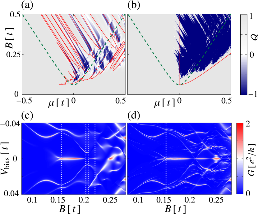
Figure 3: (a, b) Topological charge $\mathcal{Q}=\det(r)$ as a function of chemical potential $\mu$ and Zeeman splitting $B$ for a (a) short ($L=100a$) and a (b) long ($L=4000a$) disordered nanowire. Red lines are phase boundaries calculated from Eq. (8) in the main text, green dashed lines show the clean phase boundary for comparison.(c, d) The corresponding tunnel conductance for fixed $\mu=t$. Parameters in the tight-binding model were chosen to fit the Delft experiment mourik12 : Choosing the lattice spacing $a=25$nm, we obtain a hopping constant $t=\hbar^{2}/2ma^{2}=4.064$meV for the effective mass $m=0.015m_{\text{e}}$ of InSb. The short wire with $L=2.5\mu$m then corresponds to the experimental situation. The other parameters used in the simulation were $l_{\text{so}}=1/k_{\text{so}}=10a=250$nm, $\Delta=0.0615t=250\mu$eV, $\gamma=0.0492t^{2}$, and the chemical potential in the leads $\mu_{\text{leads}}=0.5t$. For the tunneling conductance in (c, d) a barrier of height $1.5t$ was added on one lattice site next to one end of the wire.

Appendix B Details of the calculation of Eq. (7)

The chiral symmetry of the Hamiltonian (5) in the main text implies that there is an operator that anti-commutes with the Hamiltonian: $\sigma_{y}\tau_{y}$. In the basis that diagonalizes this operator with degenerate blocks off-diagonalizes the Hamiltonian. In particular, we find that $U=(1+i\sigma_{x})(1+i\tau_{x})\big{(}(1+\sigma_{z})+(1-\sigma_{z})\tau_{x}\big{)}/4$ transforms the Hamiltonian to:

$$H=h(p,x)\sigma_{z}\tau_{y}-\alpha p\tau_{y}+B\sigma_{x}\tau_{x}+\Delta\tau_{x}.$$ (9)

Then the zero energy Majorana states are of either of the form $\chi_{+}=\bigl{(}{\phi_{+}\atop{0}}\bigr{)}$ or $\chi_{-}=\bigl{(}{0\atop{\phi_{-}}}\bigr{)}$, where $\phi_{\pm}$ satisfy a $2\times 2$ nonhermitian eigenvalue problem with eigenvalue zero:

$$(\mp ih(p,x)\sigma_{z}\pm i\alpha p+B\sigma_{x}+\Delta)\phi_{\pm}=0.$$ (10)

After performing a rotation in $\sigma$ space around the $x$-axis that transforms $\sigma_{z}\rightarrow\sigma_{y}$ and premultipling with $\pm\sigma_{x}$ we obtain Eq. (6) of the main text:

$$\tilde{H}\phi_{\pm}=(h(p,x)\sigma_{z}\mp B\mp\Delta\sigma_{x}-i\alpha p\sigma_{x})\phi_{\pm}=0$$ (11)

We now construct the zero energy solution for small $\alpha$. First, we perform an imaginary gauge transformation: $\phi\rightarrow e^{-\kappa_{\alpha}x}\phi$, where $\kappa_{\alpha}$ is an order $\alpha$ parameter that is yet to be determined. Then we have $p\rightarrow p+i\hbar\kappa_{\alpha}$. Next, we collect terms of order $\alpha$ and treat them as perturbations. We then have $\tilde{H}=H_{0}+H_{1}$ with

$$\!\!\!\!\!\!H_{0}=h(p,x)\sigma_{z}\mp B\mp\Delta\sigma_{x}$$ (12a)

$$\!\!\!\!\!\!H_{1}=-i\alpha p\sigma_{x}+i\frac{\hbar\kappa p}{m}\sigma_{z}+\hbar\kappa\alpha\sigma_{x}-\frac{\hbar^{2}\kappa^{2}}{2m}\sigma_{z}\,.$$ (12b)

The last two terms can be absorbed into $H_{0}$ by redefining $\mu$ and $\Delta$ and will be neglected in the following.

Zero-energy solutions of $H_{0}$ are of the form $\xi_{\pm}(\epsilon)\psi(x;\epsilon)$ where $h(p,x)\psi(x;\epsilon)=\epsilon\psi(x;\epsilon)$, $\xi_{\pm}(\epsilon)$ are the eigenvectors of the $2\times 2$ matrix $\epsilon\sigma_{z}\mp\Delta\sigma_{x}$ with eigenvalue $\pm\sqrt{\epsilon^{2}+\Delta^{2}}$, and $\epsilon=\sqrt{B^{2}-\Delta^{2}}$. $\psi(x;\epsilon)$ can be again written as a linear combination of two independent solutions $Af(x;\epsilon)+Bg(x;\epsilon)$ where we choose $f$ to be decaying and $g$ increasing.

We now choose $\kappa_{\alpha}=\mp m\alpha\Delta/\hbar\epsilon$ such that $H_{1}$ anticommutes with $\epsilon\sigma_{z}\mp\Delta\sigma_{x}$. Then, $H_{1}$ is off-diagonal in the basis of $\xi_{\pm}(x;\epsilon)$ and thus the contribution of $H_{1}$ vanishes to first order in perturbation theory. Hence,

$$\phi_{\pm}=\xi_{\pm}(\epsilon){\rm e}^{\pm\kappa x}\big{(}Af(x;\epsilon)+Bg(x;\epsilon)\big{)}$$

$$\quad\quad+\xi_{\pm}(-\epsilon){\rm e}^{\mp\kappa x}\big{(}Cf(x;-\epsilon)+Dg(x;-\epsilon)\big{)},$$ (13)

is a zero-energy solution up to order $\alpha^{2}$ with $\kappa=m\alpha\Delta/\hbar\epsilon$.

References

- (1) P. W. Anderson, Phys. Rev. Lett. 3, 325 (1959)
- (2) Abrikosov, A. A., and L. P. Gorkov, Zh. Eksp. Teor. Fiz. 39, 1781 (1960) [ Sov. Phys. JETP 12 , 1243 (1961)].
- (3) A. Y. Kitaev, Physics-Uspekhi, 44, 131(2001).
- (4) R. M. Lutchyn, J. D. Sau, S. Das Sarma, Phys. Rev. Lett. 105, 077001 (2010).
- (5) Y. Oreg, G. Refael, F. von Oppen, Phys. Rev. Lett. 105, 177002 (2010).
- (6) J. Alicea, Y. Oreg, G. Refael, F. von Oppen, and M. P. A. Fisher, Nat. Phys. 7, 412 (2011).
- (7) J. Alicea. Rep. Prog. Phys. 75, 076501 (2012)
- (8) M. Leijnse, K. Flensberg. Semicond. Sci. Technol. 27, 124003 (2012).
- (9) P.W. Brouwer, M. Duckheim, A. Romito, and F. von Oppen, Phys. Rev. B 84, 144526 (2011).
- (10) P.W. Brouwer, M. Duckheim, A. Romito, and F. von Oppen, Phys. Rev. Lett. 107, 196804 (2011).
- (11) A.C. Potter and P.A. Lee, Phys. Rev. B 83 184520 (2011), Erratum Phys. Rev. B 84, 059906(E) (2011)
- (12) J. D. Sau, S. Tewari, and S. Das Sarma, Phys. Rev. B 85, 064512 (2012).
- (13) M.-T. Rieder, G. Kells, M. Duckheim, D. Meidan, and P. W. Brouwer Phys. Rev. B 86, 125423 (2012).
- (14) M. Wimmer, A. R. Akhmerov, M. V. Medvedyeva, J. Tworzydło, and C. W. J. Beenakker, Phys. Rev. Lett. 105, 046803 (2010)
- (15) A. C. Potter and P. A. Lee, Phys. Rev. Lett. 105, 227003, (2010).
- (16) T.D. Stanescu, R.M. Lutchyn, and S. Das Sarma, Phys. Rev. B 84, 144522 (2011).
- (17) G. Kells, D. Meidan, and P.W. Brouwer, Phys. Rev. B 85, 060507(R) (2012)
- (18) V. Mourik, K. Zuo, S.M. Frolov, S.R. Plissard, E.P.A.M. Bakkers, and L.P. Kouwenhoven, Science 336, 1003 (2012)
- (19) M.T. Deng, C.L. Yu, G.Y. Huang, M. Larsson, P. Caroff, and H.Q. Xu, Nano Lett. 12, 6414 (2012)
- (20) A. Das, Y. Ronen, Y. Most, Y. Oreg, M. Heiblum, H. Shtrikman Nat. Phys. 8, 887 (2012).
- (21) J. Liu, A. C. Potter, K. T. Law, and P. A. Lee, Phys. Rev. Lett. 109, 267002 (2012).
- (22) D. Bagrets and A. Altland, Phys. Rev. Lett. 109, 227005 (2012).
- (23) D.I. Pikulin, J.P. Dahlhaus, M. Wimmer, H. Schomerus, and C.W.J. Beenakker, New. J. Phys. 14, 125011 (2012).
- (24) D. Rainis, L. Trifunovic, J. Klinovaja, and D. Loss Phys. Rev. B 87, 024515 (2013)
- (25) O. Motrunich, K. Damle, and D.A. Huse, Phys. Rev. B 63, 224204 (2001)
- (26) L.-J. Lang and S. Chen. Phys. Rev. B 86, 205135 (2012).
- (27) W. DeGottardi, D. Sen, and S. Vishveshwara, Phys. Rev. Lett. 110, 146404 (2013).
- (28) I. Adagideli, P. M. Goldbart, A. Shnirman, and A. Yazdani, Phys. Rev. Lett. 83, 5571 (1999).
- (29) Thus an unprotected pair of zero-energy modes is always accompanied by a state at the Fermi energy for the normal system, without superconductivity.
- (30) C.W.J. Beenakker, Rev. Mod. Phys. 69, 731 (1997)
- (31) A.R. Akhmerov, J.P. Dahlhaus, F. Hassler, M. Wimmer, and C.W.J. Beenakker, Phys. Rev. Lett. 106, 057001 (2011).
- (32) C.W. Groth, M. Wimmer, A.R. Akhmerov. X. Waintal. arXiv:1309.2926.
- (33) B.I. Halperin, Phys. Rev. 139, A104 (1965).
- (34) C. Itzykson and J.-M. Drouffe, Statistical Field theory 2, ch. 10, (Cambridge University Press, Cambridge, 1989).
- (35) Falko Pientka, Alessandro Romito, Mathias Duckheim, Yuval Oreg, and Felix von Oppen, New J. Phys. 15, 025001 (2013).
- (36) In Piet11 , the criterion is , with .
- (37) S. Tewari and J. D. Sau, Phys. Rev. Lett. 109, 150408 (2012)
- (38) S. Das Sarma, Jay D. Sau, and Tudor D. Stanescu Phys. Rev. B 86, 220506(R) (2012).
- (39) For a dirty wire all accidental zero mode solutions will shift under changes in the magnetic field.