Random cyclic matrices

Abstract

We present a Gaussian ensemble of random cyclic matrices on the real field and study their spectral fluctuations. These cyclic matrices are shown to be pseudo-symmetric with respect to generalized parity. We calculate the joint probability distribution function of eigenvalues and the spacing distributions analytically and numerically. For small spacings, the level spacing distribution exhibits either a Gaussian or a linear form. Furthermore, for the general case of two arbitrary complex eigenvalues, leaving out the spacings among real eigenvalues, and, among complex conjugate pairs, we find that the spacing distribution agrees completely with the Wigner distribution for Poisson process on a plane. The cyclic matrices occur in a wide variety of physical situations, including disordered linear atomic chains and Ising model in two dimensions. These exact results are also relevant to two-dimensional statistical mechanics and $\nu$-parametrized quantum chromodynamics.

With the pseudo-Hermitian extension of quantum mechanics bender ; za ; am , it has become possible to develop a number of new ideas, opening thereby interesting and important directions of investigation. One of these advances has been in random matrix theory where pseudo-unitarily invariant ensembles were presented aj that exhibit completely different kind of level repulsion as compared to the ensembles known mehta ; bipz ; ginibre . Thus, physical systems that violate parity and time-reversal invariance (${\cal PT}$-symmetric) exhibit level repulsion that could be linear or $\sim-S\log S$ where $S$ is the nearest-neighbour spacing of levels. However, an explicit analysis has been done only for an ensemble of 2 $\times$ 2 matrices.

In this Letter, we present random matrix theory (RMT) of $N\times N$ cyclic matrices with real elements. As we shall show, these matrices are pseudo-symmetric with respect to “generalized parity”. Such matrices arise in very significant contexts, the celebrated example being that of Onsager solution of two-dimensional Ising model onsager ; kaufman . They are encountered in the treatment of linear atomic chains with Born-von Kármán boundary condition lowdin1 and in understanding overlap matrices for molecules like benzene. These matrices also occur as transfer matrices in the theory of disordered chains borland and in the general context of wave propagation in one-dimensional structures luttinger . In the latter example, generally, matrices of second order occur - thus, our earlier results jain throw light on the fluctuation properties of the eigenvalues. Cyclic matrices also appear in the context of phase transitions in the spherical model spherical . In all these varied instances, as soon as there is a random parameter (e.g. external field or a random coupling in the example of Ising model), the level correlations dictate the long time tails of the time correlation functions which, in turn, relate to the relaxation of these systems when they are perturbed from thermodynamic equilibrium srjpg .

RMT appears in seemingly unrelated problems in physics and mathematics ranging from growth models, directed polymers, random sequences, to Riemann hypothesis satya ; ahmed ; jgk . Also, the study of random matrices has been related to quantum chaos and exactly solvable models in a remarkable way guhr ; jgk ; srj . Generically, the statistics of spectral fluctuations of classically integrable, pseudointegrable, and chaotic systems follow respectively the general features of Poisson, short-range Dyson model gj ; ajk or Semi-Poisson bgs , and Wigner-Dyson ensembles bohigas . However, for the physical situations occurring in two-dimensional statistical mechanics where time-reversal and parity are violated halperin ; frank ; wen ; kitazawa , there is no general understanding of the statistical nature of spectral fluctuations dj ; jd . Perhaps the first example of a billiard system with a ${\cal PT}$-symmetric (violating ${\cal P}$ and ${\cal T}$) Hamiltonian was a particle enclosed in a rectangular cavity in the presence of an Aharonov-Bohm flux line djm . For this classically pseudointegrable system, the spectral statistics of quantum energy levels was found to exhibit level repulsion that is distictly different from the standard RMT mehta . For these class of systems, an important step was taken in aj , and the present work takes us to show the nature of these fluctuations in $N\times N$ cyclic matrices. The general case of $N\times N$ random pseudo-Hermitian matrices remains open, however.

Let us consider an $N\times N$ cyclic matrix with real elements, $\{a_{i}\}$:

$$\mbox{\helv M}=\left[\begin{array}[]{cccc}a_{1}&a_{2}&...&a_{N}\\ a_{N}&a_{1}&...&a_{N-1}\\ \vdots&&&\\ a_{2}&a_{3}&...&a_{1}\end{array}\right].$$ (5)

It is important to note that this matrix is, in fact, pseudo-Hermitian (pseudo-orthogonal) with respect to $\boldsymbol{\eta}$

$$\boldsymbol{\eta}=\left[\begin{array}[]{cccccc}1&0&0&...&0&0\\ 0&0&0&...&0&1\\ 0&0&0&...&1&0\\ \vdots&&&&&\\ 0&1&0&...&0&0\end{array}\right],$$ (11)

that is,

$$\mbox{\helv M}^{\dagger}=\mbox{\helv M}^{T}=\boldsymbol{\eta}\mbox{\helv M}\boldsymbol{\eta}^{-1}.$$ (12)

Since $\boldsymbol{\eta}^{2}=$ identity, I, $\boldsymbol{\eta}$ is introduced here as “generalized parity”. Thus, we have an ensemble of random cyclic matrices (RCM) that is pseudo-orthogonally invariant in the sense of (12). There are two distinct scenario with respect to time-reversal, ${\cal T}$ and parity, ${\cal P}$: (a) standard case where ${\cal T}$ and ${\cal P}$ are preserved, this case is trivially ${\cal PT}$-symmetric, and, (b) the case of ${\cal PT}$-symmetry where ${\cal T}$ and ${\cal P}$ both are broken. In case (a), one may study the fluctuations properties of energy levels after classifying the eigenfunctions according to definite parity (odd or even); however the case (b) belongs to a different class altogether. Whereas case (a) corresponds to the invariant ensembles of random matrix theory mehta , case (b) has not been fully studied, only some partial results exist aj ; jain and RCM belong to this case. To our knowledge, the discrete symmetries for operators represented by cyclic matrices are clearly spelt out here for the first time. Due to this generality, our final results are expected to be relevant for a wide variety of physical situations occurring in anyon physics halperin , $\nu$-parametrized quantum chromodynamics, fractional quantum hall systems jkjain , etc.

The eigenvalues of M are given by kowaleski

$$E_{l}=\sum_{p=1}^{N}a_{p}\exp\frac{2\pi i}{N}(p-1)(l-1);$$ (13)

($l=1,2,...,N$), the maximum real eigenvalue being $\sum_{i}a_{i}$. The diagonalising matrix is given by spherical

$$U_{jl}=\frac{1}{\sqrt{N}}\exp\frac{2\pi i}{N}(j-1)(l-1).$$ (14)

We consider a Gaussian ensemble of cyclic matrices with a distribution,

$$P(\mbox{\helv M})\sim\exp-A~{}{\mathrm{t}r~{}}(\mbox{\helv M}^{\dagger}\mbox{\helv M})$$ (15)

where $A$ sets the scale (of energy, for instance).

For the sake of simplicity, we present the analysis for an ensemble of $3\times 3$ matrices. We would like to obtain the joint probability distribution function (JPDF) of eigenvalues because all the correlations are related to it. Also, we would like to show results on the spacing distribution as they enjoy a central place in discussions in quantum chaos, universality arguments, and rule the dominant long-time tail in correlation functions. We immediately see that ${\mathrm{t}r~{}}\mbox{\helv M}^{\dagger}\mbox{\helv M}=3(a_{1}^{2}+a_{2}^{2}+a_{3}^{2})$. In effect, we have $P(\{a_{i}\})=\left(\frac{3A}{\pi}\right)^{\frac{3}{2}}e^{-3A\sum_{i}a_{i}^{2}}$. There are three eigenvalues - one real, $E_{1}=\sum_{i}a_{i}$ and a complex conjugate pair, $(E_{2},E_{2}^{*})$. We may define spacing as $S_{23}:=|E_{2}-E_{3}|=\sqrt{3}(a_{3}-a_{2})$ as well as $S_{12}:=|E_{1}-E_{2}|=|\frac{3}{2}(a_{2}+a_{3})+\frac{i\sqrt{3}}{2}(a_{2}-a_{3})|$. Obviously, $S_{12}=S_{13}$. The JPDF of eigenvalues $P(\{E_{i}\})$ can be written as

$$P(E_{1},E_{2},E_{2}^{*})=\left(\frac{A}{\pi}\right)^{\frac{3}{2}}e^{-A(E_{1}^{2}+2|E_{2}|^{2})}.$$ (16)

With this JPDF, spacing distributions can be found note . Spacing distribution for the complex conjugate pair, $P_{cc}(S_{23})$ is given by

$$P_{cc}(S_{23}) = \int\prod_{i=1}^{3}da_{i}P(\{a_{i}\})\delta(S_{23}-\sqrt{3}|a_{3}-a_{2}|)$$ (17)

$$= \sqrt{\frac{2A}{\pi}}e^{-\frac{A}{2}S_{23}^{2}}.$$

Using this, we may define an average spacing, $\overline{S_{23}}$ through the first moment and obtain finally a normalized spacing distribution in terms of the variable $z=S_{23}/\overline{S_{23}}$:

$$p_{cc}(z)=\frac{2}{\pi}e^{-\frac{z^{2}}{\pi}}.$$ (18)

Similarly, the spacing distribution, $P_{rc}(S_{12})$ is obtained:

$$P_{rc}(S_{12})=\frac{4A}{\sqrt{3}}S_{12}e^{-\frac{4}{3}S_{12}^{2}}I_{0}\left(\frac{2}{3}AS_{12}^{2}\right).$$ (19)

Mean spacing turns out to be $\overline{S_{12}}=\frac{3}{8}\sqrt{\frac{\pi}{A}}c$ where $c=~{}_{2}F_{1}\left[\frac{3}{4},\frac{5}{4},1,\frac{1}{4}\right]=1.31112...$ Defining $z=S_{12}/\overline{S_{12}}$,

$$p_{rc}(z) = \frac{3\sqrt{3}\pi}{16}c^{2}z\exp\left(-\frac{3\pi}{16}c^{2}z^{2}\right)$$ (20)

$$I_{0}\left(\frac{3\pi}{32}c^{2}z^{2}\right).$$

We can now make following observations : (i) the Gaussianity of $p_{cc}(z)$ implies that there is no level repulsion among the complex conjugate pairs, at the same time there is no attraction, there is no tendency of clustering as in Poissonian spacing distribution; (ii) real and complex eigenvalues display linear level repulsion. These results are also borne out by the numerical simulations in Fig. 1 and Fig. 2.

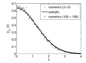
Figure 1: Probability distribution of the absolute spacing between the complex conjugate pair of eigenvalues of a Gaussian ensemble of $3\times 3$ cyclic matrices. The numerical result obtained by considering 10000 realizations agrees with the analytic result (18). The Gaussian spacing distribution may be interpreted to give an accumulation of eigenvalues resulting in a maximum at zero spacing, but no tendency to cluster as the first derivative is zero. This is different from a Poisson distribution.

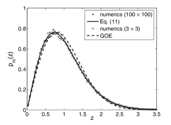
Figure 2: Probability distribution of the absolute spacing between a real and a complex eigenvalue of a Gaussian ensemble of $3\times 3$ cyclic matrices. The numerical result obtained by considering 10000 realizations for $3\times 3$ matrices and 1000 realizations of $100\times 100$ matrices agrees with the analytic result (20). We observe a linear level repulsion near zero spacing, however the result is distinctly different from the Wigner surmise for GOE.

For the general case of $N\times N$ matrices, we need to invert (13). This inversion leads us to the following relation:

$$a_{i}=\sum_{l}\mbox{\helv S}_{il}E_{l}$$ (21)

where S_il = $\omega^{(i-1)(N-(l-1))}$ and $\omega=e^{2\pi i/N}$ is a root of unity. S is a symmetric matrix and S${}^{2}=N\boldsymbol{\eta}$. Employing these relations, we can find $\sum_{i}a_{i}^{2}$, and hence the following result for the JPDF for even $N$:

$$P(\{E_{i}\}) = \left(\frac{A}{\pi}\right)^{\frac{N}{2}}\exp\bigg{[}-A\bigg{(}E_{1}^{2}+E_{\frac{N}{2}+1}^{2}$$ (22)

$$~{}~{}~{}~{}~{}+\sum_{i\neq 1,\frac{N}{2}+1}^{N}E_{i}E_{N+2-i}\bigg{)}\bigg{]}$$

where $E_{1}$ and $E_{\frac{N}{2}+1}$ real and the rest of the eigenvalues may be complex. For odd $N$, the above result will hold except that there will be only one real eigenvalue, $E_{1}$ and the summation in the second term will extend over all $i$ except 1. Employing this general result on JPDF, we can now calculate the spacing distributions for the general case. There are three cases : (i) spacing among the complex conjugate pair of eigenvalues is found to be distributed again as a Gaussian; (ii) spacing between a real and a complex eigenvalue is distributed according to (20); (iii) two complex eigenvalues, $E_{j}=x_{j}+iy_{j}$ and $E_{k}=x_{k}+iy_{k}$ are spaced according to

$$p(s)=\frac{\int\prod_{i}d\Re{E_{i}}d\Im{E_{i}}P(\{E_{i}\})\delta(|E_{j}-E_{k}|-s)}{\int\prod_{i}d\Re{E_{i}}d\Im{E_{i}}P(\{E_{i}\})},$$ (23)

which reduces to the following integral on change of variables, $\xi(\eta)_{\pm}=x(y)_{k}\pm x(y)_{j}$

$$p(s) = \frac{A}{\pi}\int d\xi_{-}d\eta_{-}e^{-A(\xi_{-}^{2}+\eta_{-}^{2})}\delta(\sqrt{\xi_{-}^{2}+\eta_{-}^{2}}-s)$$ (24)

$$= \frac{\pi s}{2}\exp\left(-\frac{\pi s^{2}}{4}\right)$$

which is exactly the Wigner distribution (Fig. 3). Let us recall that Wigner’s result holds exactly for $2\times 2$ real symmetric matrices, it serves as an excellent approximation for $N\times N$ matrices though. We also know that the spacing distribution for a Poissonian random process in a plane is exactly the same as Wigner surmise. Thus our result proves that the complex eigenvalues of random cyclic matrices describe such a process. This is a very beautiful, non-intuitive result which brings out yet another characteristic of RCM.

Figure 3: We observe a linear level repulsion between two eigenvalues which are neither real nor complex conjugate pairs for an ensemble of $100\times 100$ matrices with 5000 realizations. The agreement with GOE is deceptive; in fact, this suggests that the eigenvalues describe a Poisson process on a plane.

The eigenfunctions of M corresponding to the real eigenvalues ($E_{1}$ and $E_{\frac{N}{2}+1}$) are also simultaneously eigenfunctions of “generalized parity” $\boldsymbol{\eta}$. However, the eigenfunctions of M corresponding to the complex conjugate pair of eigenvalues are not simultaneously eigenfunctions of $\boldsymbol{\eta}$. Thus, when these complex eigenvalues occur, “generalized parity” is said to be spontaneously broken. Also, the eigenfunctions corresponding to the complex conjugate pair of eigenvalues have zero ${\cal PT}$ - norm. This is expected from the recent works bender ; ahmed on ${\cal PT}$-symmetric quantum mechanics. This observation then fully embeds our findings into the new random matrix theory developed recently for pseudo-Hermitian Hamiltonians. However, we also note that the eigenvectors $\psi_{1}$ ($\psi_{2}$) corresponding to complex conjugate eigenvalues, $\lambda$ ($\lambda^{*}$) satisfy orthogonality defined with respect to $\boldsymbol{\eta}$. Since these results are found for $N\times N$ matrices, we believe that this work extends the random matrix theory in a significant way. The findings on the spacing distributions have led us to a linear level repulsion among distinct complex eigenvalues, whereas the spacing between complex-conjugate pair is Gaussian-distributed.

Ginibre orthogonal ensemble with Gaussian distributed real elements has been completely solved only recently Kanzieper ; Peter . The ensemble of asymmetric random cyclic matrices is a simple nontrivial instance for which all the interesting quantities are analytically obtained in an explicit manner. Such examples play an important role in developing a deeper insight, even when formal results exist.

Also, we would like to point out the role played by level repulsion when a system with spectral properties described by RMT approaches equilibrium. In its approach to equilibrium, the central quantity of interest is the two-time correlation function, the long-time behaviour is decided by the degree of level repulsion as the levels get closer. We can immediately see srjpg that linear level repulsion is related to the exponent, 2 in $t^{-2}$-tail at long times.

It is a great pleasure to thank Bob Dorfman, University of Maryland, College Park, U.S.A. for bringing to our notice the role played by cyclic matrices in certain models in statistical mechanics, the work of Ted Berlin and Mark Kac spherical in particular.

References

- (1) C. M. Bender, D. C. Brody, and H. F. Jones, Phys. Rev. Lett. 89 (2002) 270401.
- (2) Z. Ahmed, Phys. Lett. A 294 (2002) 287.
- (3) A. Mostafazadeh, J. Math. Phys. 43 (2002) 3944.
- (4) Z. Ahmed and S. R. Jain, Phys. Rev. E67 (2003) 045106(R).
- (5) M. L. Mehta, Random matrices (Academic Press, London, 1991).
- (6) E. Brèzin, C. Itzykson, G. Parisi, and J.-B. Zuber, Commun. Math. Phys 59(1978) 35.
- (7) J. Ginibre, J. Math. Phys. 6 (1965) 440.
- (8) L. Onsager, Phys. Rev. 65, (1944) 117.
- (9) B. Kaufman, Phys. Rev. 76, (1949) 1232.
- (10) P. O. Löwdin, R. Pauncz, and J. de Heer, J. Math. Phys. 1, (1960) 461.
- (11) R. E. Borland, Proc. Phys. Soc. (London) 83, (1964) 1027.
- (12) J. M. Luttinger, Philips Research Rep. 6, (1951) 303.
- (13) Z. Ahmed and S. R. Jain, J. Phys. A36, (2003) 3349.
- (14) T. H. Berlin and M. Kac, Phys. Rev. 86, (1952) 821.
- (15) S. R. Jain and P. Gaspard, “Time correlation functions in complex quantum systems” (preprint); S. R. Jain, Nonlinear dynamics and computational physics, ed. V. B. Sheorey (Narosa, New Delhi, 1999).
- (16) S. N. Majumdar, arXiv:cond-mat/0701193 [cond-mat.stat-mech]; P. Deift, math-ph/0603038.
- (17) Z. Ahmed and S. R. Jain, Mod. Phys. Lett. 21, (2006) 331.
- (18) S. R. Jain, B. Grémaud, and A. Khare, Phys. Rev. E66, (2002) 016216.
- (19) T. Guhr, A. Müller-Groeling, H. A. Weidenmüller, Phys. Rep. 299 , (1998) 189.
- (20) S. R. Jain, Czech. J. Phys. 56, (2006) 1021.
- (21) B. Grémaud and S. R. Jain, J. Phys. A , (1998) L631.
- (22) G. Auberson, S. R. Jain, and A. Khare, J. Phys. A 34, (2001) 695.
- (23) A. Pandey (unpublished); E. Bogomolny, U. Gerland, and C. Schmit, Phys. Rev. E 59, (1999) 1315 (R).
- (24) O. Bohigas, M.-J. Gianonni, and C. Schmit, Phys. Rev. Lett. 52, (1984) 1.
- (25) A. Lerda, Anyons Lecture notes in Physics (m-14) (Springer, New York, 1992).
- (26) J. K. Jain, Phys. Today (April 2000) p. 39.
- (27) B. I. Halperin, J. March Russel, and F. Wilczek, Phys. Rev. B40, 8726 (1989).
- (28) X. G. Wen and A. Zee, Phys. Rev. Lett. 62, 2873 (1989).
- (29) Y. Kitazawa, Phys. Rev. Lett. 65, 1275 (1990).
- (30) D. Alonso and S. R. Jain, Phys. Lett. B 387, (1996) 812.
- (31) S. R. Jain and D. Alonso, J. Phys. A 30, (1997) 4993.
- (32) G. Date, S. R. Jain, and M. V. N. Murthy, Phys. Rev. E 51, (1995) 198.
- (33) G. Kowaleski, Determinantentheorie (Chelsea, New York, 1948), third edition.
- (34) Note that we are not using the term “nearest neighbour spacing distribution” because the spacings are in general complex.
- (35) E. Kanzieper and G. Akemann, Phys. Rev. Lett.95, (2005) 230201.
- (36) P. J. Forrester and T. Nagao, Phys. Rev. Lett.99, (2007) 050603.