Orbital parameters, chemical composition, and magnetic field of the Ap binary HD 98088

Abstract

HD 98088 is a synchronised, double-lined spectroscopic binary system with a magnetic Ap primary component and an Am secondary component. We study this rare system using high-resolution MuSiCoS spectropolarimetric data, to gain insight into the effect of binarity on the origin of stellar magnetism and the formation of chemical peculiarities in A-type stars. Using a new collection of 29 high-resolution Stokes $VQU$ spectra we re-derive the orbital and stellar physical parameters and conduct the first disentangling of spectroscopic observations of the system to conduct spectral analysis of the individual stellar components. From this analysis we determine the projected rotational velocities of the stars and conduct a detailed chemical abundance analysis of each component using both the Synth3 and Zeeman spectrum synthesis codes. The surface abundances of the primary component are typical of a cool Ap star, while those of the secondary component are typical of an Am star. We present the first magnetic analysis of both components using modern data. Using Least-Squares Deconvolution, we extract the longitudinal magnetic field strength of the primary component, which is observed to vary between +1170 and -920 G with a period consistent with the orbital period. There is no field detected in the secondary component. The magnetic field in the primary is predominantly dipolar, with the positive pole oriented approximately towards the secondary.

1 Introduction

Ap stars are magnetic intermediate-mass main sequence stars that exhibit distinctive chemical peculiarities in their atmospheres. Although other classes of chemically peculiar stars exist (e.g. Am stars, Hg-Mn stars), these stars have been demonstrated to lack strong, organised magnetic fields at their surfaces (e.g. Shorlin et al., 2002; Wade et al., 2006; Makaganiuk et al., 2011). Ap stars appear to be the only class of middle main-sequence stars for which, in all cases, an observable magnetic field is present (Aurière et al., 2007).

The magnetic fields of Ap stars have been established to have important global dipole components ranging in strength from hundreds to tens of thousands of gauss. The symmetry axis of the dipole component is almost always tilted relative the stellar rotation axis. In addition, Ap stars generally spin much more slowly than non-peculiar stars of similar masses (Abt & Morrell, 1995; Stȩpień, 2000), and as they spin they exhibit line profile variations attributed to rotational modulation of patchy, non-axisymmetric lateral and vertical distributions of chemical abundance in their photospheres. While it is generally accepted that the fundamental mechanism responsible for the chemical peculiarities is microscopic chemical diffusion (as described by Michaud 1970), the origin of chemical patchiness, and the relationship to the magnetic field, is poorly understood.

Although modern surveys (Gerbaldi et al., 1985; Carrier et al., 2002) indicate that Ap stars exhibit about the same binary frequency as normal A-type stars ($47\pm 5$%, Jaschek & Gómez, 1970), they generally agree that there is a clear lack of Ap stars in short-period (i.e. $P_{\rm orb}=3.0$ days or less) systems (Carrier et al., 2002). One might hypothesize that this could be because these systems tend to be synchronized. Such a short-period binary would imply a short rotational period for both components. Rapid rotation would induce rotational mixing, inhibiting the development of chemical peculiarities. However, no similar absence of short period systems exists for Am binaries. This suggests that binaries with short periods are capable of hosting chemically peculiar stars, but contain few magnetic (chemically peculiar) stars. The few magnetic Ap stars reported to be in short period binaries could therefore be very interesting targets for studying the origin and evolution of magnetic fields in intermediate-mass stars.

Systems containing two A-type stars are of particular interest, since they provide an opportunity for studying not only the incidence and evolution of stellar magnetic fields, but also of chemical peculiarity in both stellar components. A comprehensive literature review reveals that these ideal systems are indeed very rare. Both HD 135728 (Freyhammer et al., 2008) and HD 59435 (Wade et al., 1999) have magnetic Ap secondary components; however their primary components are giants of spectral type G8. While these primary giant G8 stars evolved from main sequence stars with masses similar to that of the Ap star, the evolved primary component makes these systems less useful to study. There are only five reported SB2 binaries with a magnetic Ap primary component and a main sequence A star companion. The first of these systems is HD 55719, which was studied by Bonsack (1976), although as a southern object it has received relatively less attention in the modern literature. HD 5550, HD 22128, and HD 56495 (e.g. Carrier et al., 2002) show composite A-type spectra, although the magnetic nature of the Ap component has yet to be definitively established. The final system is HD 98088, which is the subject of this paper. This system is very well-suited for the study of magnetic fields and chemical peculiarities, and is one of the brightest and best-studied magnetic binary systems.

HD 98088 (HR 4369, HIP 55106) was first observed as a spectroscopic binary by Abt (1953), although he reported it to be an SB1. The primary radial velocity was found to vary with an orbital period of $5.905\pm 0.005$ days. Spectrophotometric analysis using the Mills spectrograph showed variability in beryllium and titanium lines. Five years later Babcock (1958) confirmed the presence of a magnetic field in HD 98088 using polarized spectroscopy. The strength of the longitudinal magnetic field was found to vary between $-1000$ and $+800$ gauss with a period consistent with the orbital period derived by Abt (1953). These measurements made HD 98088 the first observed synchronized spectroscopic binary containing a magnetic star (Babcock, 1958). In his 1965 paper on spectral classification, Osawa classified the Ap primary star to be of spectral subtype SrCr.

The first complete orbital solution of this SB2 system was computed by Abt et al. (1968). Abt et al. (1968) searched for photometric eclipses without success. From the the difference in equivalent widths of the Ca ii K, Mg ii ${\lambda}4481$, Na i D₁ and D₂, Si ii ${\lambda}6371$, and H${\alpha}$ lines, the magnitude difference of the components were estimated to be ${\Delta}m_{V}=1.2$. This led them to conclude that the primary has spectral type A3Vp and the secondary has spectral type A8V. The masses of each component were then inferred from the spectral type, and combined with the dynamic $M{\sin}^{3}i$ to determine the system’s inclination angle $i=67\degr$. An interesting feature discovered by Abt et al. (1968) is that despite its short orbital period, HD 98088 has significant orbital eccentricity. This suggests that apsidal motion should take place. However, Wolff (1974) obtained new spectroscopic observations that were used in conjunction with older measurements to refine the period of apsidal motion to at least 700 years.

Carrier et al. (2002) reobserved the system using the CORAVEL velocimeter. With these measurements, and all other published radial velocity measurements of the system, the orbital period of HD 98088 was refined to $5.905111\pm 0.000004$ days. The Carrier et al. (2002) solution is consistent with the solution of Abt et al. (1968). Carrier et al. (2002) observed no significant variation of the longitude of periastron, and concluded that the apsidal period is longer than one millennium. They used the Hipparcos distance and effective temperatures determined from Geneva photometry to derived the masses of the components from their HR diagram positions to be $M_{1}=2.261\pm 0.093$ $M_{\odot}$ and $M_{2}=1.677\pm 0.085$ $M_{\odot}$. Assuming negligible Zeeman broadening and a synchronized system, they found the radii to be $R_{1}=3.27\pm 0.43$ $R_{\odot}$ and $R_{2}=2.10\pm 0.28$ $R_{\odot}$ using the projected rotational velocities and the orbital period. The inclination angle was found to be $i=66^{\circ}$ by comparing the minimum dynamical masses to the evolutionary masses.

The HD 98088 system potentially provides a very interesting and rare insight into chemical peculiarities and magnetism in A type stars, in the context of close binary systems. The similarities between the physical parameters of the primary and secondary make it an excellent laboratory for comparative astrophysics. In this paper we use spectroscopic and polarimetric data to improve the orbital parameters of the system, to perform a detailed abundances analysis of the spectra of both stellar components, and to analyze the magnetic properties of the system.

2 Observations

Observations of HD 98088 were obtained with the Multi-Site Continuous Spectroscopy (MuSiCoS) spectropolarimeter, a now-decommissioned high resolution spectropolarimeter located at the the Télescope Bernard Lyot at the Observatoire du Pic du Midi, France. The instrument consists of a bench mounted cross-dispersed échelle spectrograph (Baudrand & Bohm, 1992), fibre-fed from a Cassegrain mounted polarimeter unit (Donati et al., 1999). The instrument provides continuous wavelength coverage from about 4500 to 6500 Å  at a resolution of $R=35\,000$. Observations were obtained in spectropolarimetric mode, providing Stokes $V$, $Q$ and $U$ spectra as well as Stokes $I$ spectra. The data were reduced using the ESpRIT (Donati et al., 1997) reduction tool, which performs relevant calibrations and optimal 1D spectrum extraction.

A total of 29 spectra - 10 Stokes $V$, 10 Stokes $Q$ and 9 Stokes $U$ - were obtained between Jan 1999 and Jan 2002. A summary of the observations is presented in Table 1. The typical signal-to-noise ratio (S/N) per 4.5 km/s spectral pixel was about 170 for Stokes $V$ and 230 for Stokes $Q/U$. The orbital phases are calculated with the ephemeris described in Table 2.

Least-Squares Deconvolution (LSD) was applied to each of the calibrated and normalised spectra. Line masks were constructed using the derived atmospheric parameters (determined in Sect. 5) and abundances (derived in Sect. 6) of both the primary and secondary components. Due to the similarity between the temperatures and abundances of the two stars, only small differences were observed in the profiles obtained from the two lines masks. Ultimately, we decided to use only the line mask corresponding to the primary to extract the LSD profiles.

All LSD profiles are normalised to a wavelength of 525 nm and a landé factor of 1.41, corresponding approximately to the S/N-weighted mean of the observed lines included in the mask.

Table 1: Summary of MuSiCoS observations. The UT date, the Julian Date, the Stokes parameter, and the peak signal to noise ratio are given. The orbital phase of the observation was calculated using the ephemeris described in Table 2. Since the system appears to be synchronized, the rotational phase is assumed to be equal to the orbital phase. For each observation, four subexposures of $300$s duration were acquired.

Date	HJD	Phase	Stokes	Peak	Velocity (km s-1)
	(2,450,000+)		Param	S/N	Primary	Secondary
Jan 18, 1999	1197.617	0.358	$V$	190	-8.0 $\pm$ 2.2
Jan 18, 1999	1197.643	0.362	$Q$	240	-9.2 $\pm$ 2.3
Jan 18, 1999	1197.674	0.368	$U$	230	-6.3 $\pm$ 2.2
Jan 23, 1999	1202.590	0.200	$V$	140	52.5 $\pm$ 2.6	-84.7 $\pm$ 1.5
Jan 23, 1999	1202.617	0.205	$Q$	210	53.7 $\pm$ 2.7	-85.9 $\pm$ 1.5
Jan 24, 1999	1203.555	0.364	$V$	180	-8.9 $\pm$ 2.2
Jan 24, 1999	1203.581	0.368	$Q$	200	-9.9 $\pm$ 2.3
Jan 24, 1999	1203.613	0.374	$U$	200	-7.7 $\pm$ 2.2
Mar 05, 2000	1609.524	0.112	$V$	190	77.5 $\pm$ 2.2	-118.7 $\pm$ 0.9
Mar 07, 2000	1611.519	0.450	$Q$	230	-33.7 $\pm$ 2.2	34.1 $\pm$ 0.5
Mar 07, 2000	1611.554	0.456	$U$	240	-35.3 $\pm$ 2.3	34.5 $\pm$ 0.5
Dec 05, 2001	2249.685	0.520	$V$	100	-53.2 $\pm$ 2.4
Dec 05, 2001	2249.710	0.525	$Q$	160	-54.0 $\pm$ 2.4
Dec 05, 2001	2249.742	0.530	$U$	130	-52.5 $\pm$ 2.4
Dec 07, 2001	2251.693	0.860	$Q$	270	-28.6 $\pm$ 2.3	29.1 $\pm$ 1.6
Dec 07, 2001	2251.725	0.866	$U$	250	-25.5 $\pm$ 2.4
Dec 07, 2001	2251.751	0.870	$V$	180	-23.3 $\pm$ 2.5
Dec 08, 2001	2252.690	0.029	$Q$	230	65.8 $\pm$ 2.4	-101.7 $\pm$ 1.8
Dec 08, 2001	2252.722	0.035	$U$	230	67.3 $\pm$ 2.2	-103.8 $\pm$ 2.5
Dec 08, 2001	2252.748	0.039	$V$	160	68.8 $\pm$ 2.5	-107.0 $\pm$ 1.4
Dec 09, 2001	2253.687	0.198	$Q$	250	54.3 $\pm$ 2.8	-86.0 $\pm$ 2.6
Dec 09, 2001	2253.715	0.203	$U$	240	52.9 $\pm$ 2.5	-85.0 $\pm$ 1.8
Dec 09, 2001	2253.750	0.209	$V$	230	50.6 $\pm$ 2.8	-84.4 $\pm$ 1.1
Dec 12, 2001	2256.710	0.710	$Q$	270	-71.5 $\pm$ 2.6	83.0 $\pm$ 5.6
Dec 12, 2001	2256.741	0.715	$U$	250	-71.3 $\pm$ 2.6	82.5 $\pm$ 2.8
Dec 12, 2001	2256.762	0.719	$V$	110	-71.2 $\pm$ 2.6	82.0 $\pm$ 1.8
Jan 05, 2002	2280.694	0.772	$Q$	230	-63.2 $\pm$ 2.5
Jan 05, 2002	2280.731	0.778	$U$	200	-61.3 $\pm$ 2.4
Jan 05, 2002	2280.759	0.783	$V$	130	-60.5 $\pm$ 2.4

3 Orbit

Orbital parameters for HD 98088 were determined using new and previously published measurements of the radial velocities of both the primary and secondary components. Published data are from Abt (1953), Abt et al. (1968), Wolff (1974), and Carrier et al. (2002). The new radial velocities measurements were obtained using the LSD profiles discussed in the previous section, extracted from each of the reduced spectra. To measure the radial velocities of the LSD line profiles of each component we used an IDL code, described by Alecian et al. (2008), that fits the binary profile by least-squares using the IDL function CURVEFIT. The binary profile is assumed to be the sum of two photospheric functions, one for each component of the system. Each photospheric function is the convolution of a rotation profile and a Gaussian of instrumental and turbulent velocity width (Gray, 2005). For the purpose of the fit, the turbulent velocity was fixed at 2 km s^-1, and the rotation profile broadening was left as a free parameter. The errors were calculated using a Monte-Carlo-type approach in which five thousand observed profiles were calculated by adding random noise to the best fit profile. The fitting procedure was repeated on each of these five thousand profiles and the standard deviation of these measurements was adopted as the error. The derived radial velocities are reported in Table 1.

The full set of radial velocity measurements was used to determine orbital parameters for the binary system. This was done by fitting orbital radial velocity curves to the measured velocities. A small constant offset between our values and Carrier et al. (2002) was used ($\approx 2$ km s^-1), significantly improving our fit to the radial velocities, following the work of Carrier et al. (2002) who found it necessary to shift their radial velocities with respect to previous measurements. The best fit orbital parameters are presented in Table 2, and the fit to the radial velocities is shown in Fig. 1. Our orbital parameters are consistent with those of Carrier et al. (2002), although our parameters are more precise due to our larger dataset.

Table 2: Best fit orbital parameters, allowing for offsets between the radial velocities of Carrier et al. (2002) and older measurements ($\Delta v_{1}$), and between our measurements and older values ($\Delta v_{2}$).

Reduced $\chi^{2}$	1.2039
RMS(A)	2.1863
RMS(B)	6.9670
$P$ (d)	$5.9051102\pm 0.0000023$
$T_{0}$ (HJD -2,400,000)	$34401.369\pm 0.015$
$K_{\rm A}$ (km s-1)	$73.31\pm 0.26$
$K_{\rm B}$ (km s-1)	$100.70\pm 0.43$
$V_{0}$ (km s-1)	$-8.65\pm 0.29$
$e$	$0.1840\pm 0.0025$
$\omega$ ($\degr$)	$313.25\pm 0.89$
$\Delta v_{1}$ (km s-1)	$-1.34\pm 0.38$
$\Delta v_{2}$ (km s-1)	$-3.02\pm 0.40$
$M_{\rm A}/M_{\rm B}$	$1.374\pm 0.008$
$M_{\rm A}\sin^{3}i$ ($M_{\odot}$)	$1.772\pm 0.013$
$M_{\rm B}\sin^{3}i$ ($M_{\odot}$)	$1.2897\pm 0.0089$
$a_{\rm A}\sin i$ ($R_{\odot}$)	$8.411\pm 0.030$
$a_{\rm B}\sin i$ ($R_{\odot}$)	$11.553\pm 0.050$

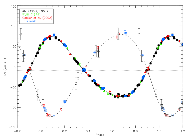
Figure 1: Measured radial velocities for the primary (full symbols) and secondary (empty symbols), phased with the orbital period of $5.9051102\pm 0.0000023$ days. Also shown is the best fit orbital curve to those velocities for the primary (solid line) and secondary (dashed line), using the ephemeris from Table 2.

4 Spectral Disentangling

The spectra of HD 98088 exhibit a complex pattern of two similar absorption line systems, with velocity separation changing from zero to $\sim$200 km s^-1 and a period on the time scale of 5.9 days. In addition, one of the components has significant intrinsic line profile variability. In this situation a spectral disentangling procedure is essential to separate this effect from variable line blending due to orbital motion of the binary components and to obtain high-quality average spectra for abundance analysis.

We employ the direct spectral decomposition technique discussed by Folsom et al. (2010). Our algorithm operates in an iterative fashion, as follows. We begin with a set of approximate radial velocities for each component and initial guesses of their spectra. Then the contribution of the less luminous component B is subtracted from the observed spectra, and all spectra are shifted to the rest frame of component A. The spectra are interpolated on a standard wavelength grid and co-added, yielding a new approximation of the primary spectrum. The same procedure is then used to update the approximation of the secondary spectrum. This sequence of operations is repeated up to convergence. Once converged spectra for the two components have been found the second part of the algorithm begins. In this part we use a least-squares minimisation routine to derive improved radial velocities (if desired) and correct the continuum normalisation of the individual spectra using low-degree polynomials (up to this point the program does not distinguish between lines and continuum). The first part of the program calculating disentangled spectra and the second part of the program fitting radial velocities are alternated until the changes in parameters from one iteration to the next are below given thresholds.

This spectral disentangling was applied to overlapping 45 Å segments of the spectra from 4500 Å to 6590 Å. While this wavelength range includes the H$\alpha$ and H$\beta$ Balmer lines, disentangling does not produce useful results for these lines. This is because the radial velocity variation between the components of HD 98088 is insufficient to disentangle such broad lines, and because automatic continuum normalisation of these broad features can be inaccurate. The radial velocities used were measured from the LSD profiles, presented in in Table 1, and were not refined in the disentangling process due to intrinsic variability of the line profiles in the primary.

Disentangling yields separate averaged high-quality ($S/N\approx 1000$) spectra of components A and B, as well as standard deviation curves which characterise the remaining discrepancy between the observations and composite model spectra. The standard deviation can be examined in the rest frame of the primary and secondary separately. A coherent excess in the standard deviation corresponding to a certain absorption feature provides a straightforward, objective identification of intrinsic variability in that line. Performing this comparison, we found that all cases of intrinsic spectrum variability were associated with the lines of HD 98088 A. Variability in the primary was found in lines of Cr, Ba, Nd, and Eu, with weaker variability in lines of Mn and Sc. No clear variability was found in other lines, at the level of the noise in our spectra.

5 Fundamental Parameters

The luminosity ratio of HD 98088 was estimated using the H$\alpha$ Balmer line cores. While the Balmer lines wings of the two components of HD 98088 are heavily blended, the cores are clearly separated in most of our observations. The depths of the H$\alpha$ cores are only weakly dependent on temperature, and thus can be used to estimate the flux ratio of HD 98088 A to HD 98088 B at 6560 Å.

To model the H$\alpha$ line cores, we began with the $T_{\rm eff}$ and $\log\,{g}$ estimates from Carrier et al. (2002). Rather than using synthetic H$\alpha$ profiles, which can have inaccurate cores due to significant non-LTE effects, we used observed H$\alpha$ profiles of the single stars HD 108651 and HD 73709. The stars were observed by Shorlin et al. (2002) with MuSiCoS and have similar parameters to HD 98088 A (HD 108651: $T_{\rm eff}$ $=8100$ K, $\log\,{g}$ $=4.36$, $v\sin i$ $=23$ km s^-1; HD 73709: $T_{\rm eff}$ $=8080$ K, $\log\,{g}$ $=4.02$, $v\sin i$ $=22$ km s^-1; Shorlin et al. 2002). Observations of the two stars were averaged to produce our model H$\alpha$ line core. A composite binary H$\alpha$ line was constructed by adding two model H$\alpha$ lines, appropriately Doppler shifted, weighted by the flux ratio at 6560 Å. This was then fit to the observed H$\alpha$ line in the binary spectrum by varying the flux ratio. This was repeated for seven observations, producing values of $F_{A}/F_{B}$ of 3.0 to 3.3. An uncertainty was estimated by the range of values allowed by the noise in our observations, and our final best value is $F_{A}/F_{B}=3.1\pm 0.2$. An example of a fit to the H$\alpha$ line core of an observation is given in Fig. 2.

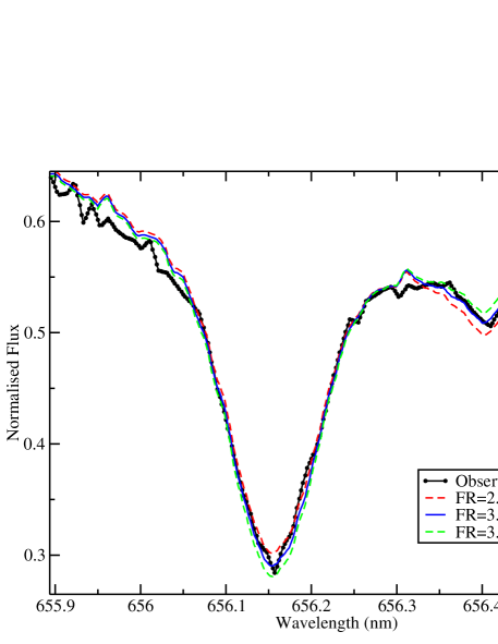
Figure 2: Sample fits to the observed combined H$\alpha$ core of HD 98088, for our best fit flux ratio at 6560 Å (FR) of 3.1, and for two other flux ratios at $\pm 2\sigma$.

The flux ratio at 6560 Å was then converted into a (bolometric) luminosity ratio by comparing with synthetic ATLAS9 flux distributions (Kurucz, 1993) for the atmospheric parameters in Table 3 at 6560 Å, and assuming $L_{\rm A}/L_{\rm B}=(T_{\rm eff,A}/T_{\rm eff,B})^{4}(R_{\rm A}/R_{\rm B})^{2}$. This was done iteratively with the determination of effective temperature and surface gravity, discussed below. Using our final $T_{\rm eff}$, 8300 K for the primary and 7500 K for the secondary, this produces $L_{\rm A}/L_{\rm B}=3.62\pm 0.72$ and $R_{\rm A}/R_{\rm B}=1.55\pm 0.05$.

Effective temperatures for both components of HD 98088 were determined from the spectral energy distribution (SED) of the system, since the Balmer lines were heavily blended. Since the system is not spatially resolved, simple photometry of the system is insufficient to determine the temperatures of both stars.

Optical spectrophotometry was taken from the database of Adelman et al. (1989). Photometry in the UV was based on observations from the TD1 satellite, as presented by Thompson et al. (1978). IR photometry was taken from the Two Micron All Sky Survey (2MASS) (Skrutskie et al., 2006). Synthetic model fluxes were taken from ATLAS9 models. Enhanced abundances ($10\times$ solar) were used to reflect the chemically peculiar nature of the primary and, as we will show, the secondary. Both the models and the observations were normalised to the flux at 5000 Å, and are presented in magnitudes. The model fluxes were added, weighted by the luminosity ratio.

Since HD 98088 is nearby ($129.5\pm 6.7$ pc) reddening of system is likely very small, and has thus been neglected in our analysis. The reddening maps of Lucke (1978) suggests that $E(B-V)<0.02$. The detailed maps of Schlegel et al. (1998), which include all Galactic reddening along a line of sight, puts an upper limit on the reddening of $E(B-V)<0.05$, though the true value for the HD 98088 system is likely much less. Thus, following the recommendation of Lipski & Stȩpień (2008), since the reddening is small we neglect it.

Fitting the SED provided well constrained effective temperatures for both stars. Since the primary dominates the flux in the UV, and the secondary’s flux nearly matches the primary in the IR, precise $T_{\rm eff}$ values for both stars can be derived. However, surface gravity cannot be determined simultaneously for both stars with the same precision, since $\log\,{g}$ predominately affects the Balmer jump where flux from both stars is important. The luminosity weighted mean $\log\,{g}$ is 4.0, but there is a mild degeneracy between the two stars. The fit to the observed SED is presented in Fig. 3, and the best fit parameters for the primary are $T_{\rm eff}$ $=8300\pm 300$ K and $\log\,{g}$ $=4.0\pm 0.5$, and for the secondary $T_{\rm eff}$ $=7500\pm 300$K and $\log\,{g}$ $=4.0\pm 0.5$.

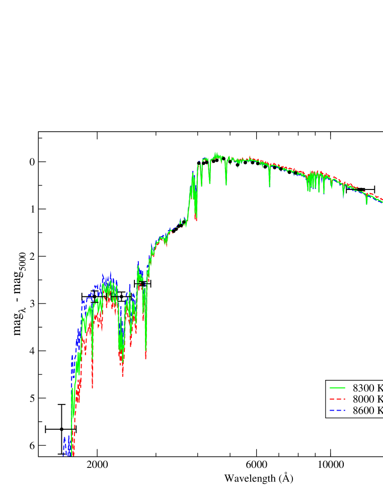
Figure 3: Fits to the spectrophotometric data using model binary flux distributions. The models are labelled by the $T_{\rm eff}$ of the primary and secondary, all for $\log\,{g}$$=4.0$ and a luminosity ratio of 3.6. The error bars in wavelength represent the full width of the filters for the UV and IR photometry.

HD 98088 was observed with Hipparcos, allowing us to determine accurate luminosities. Based on the new reduction by van Leeuwen (2007), the system has a parallax of $7.72\pm 0.4$ mas and a $V$ magnitude of $6.173\pm 0.007$. The uncertainty in magnitude is the standard deviation of the Hipparcos measurements rather than the (substantially smaller) quoted formal uncertainty, and agrees with the $b$ and $y$ band photometric variability found by Catalano & Leone (1994). The bolometric correction for Ap stars from Landstreet et al. (2007) was used, since we find both components of HD 98088 have strong peculiarities, producing $BC_{\rm A}=0.08$ and $BC_{\rm B}=0.09$ (we adopted $M_{\rm bol,\odot}=4.74$). For comparison, the bolometric correction of Balona (1994) produces $BC_{\rm A}=0.01$ and $BC_{\rm B}=0.04$. Following the recommendation of Landstreet et al. (2007), we adopted a conservative uncertainty on the bolometric correction of 0.1 in order to account for any potential systematic uncertainties. Using the luminosity ratio we calculated the bolometric magnitude difference between the primary and the total system ($m_{\rm A}-m_{\rm tot}=0.265\pm 0.053$), and the difference between the secondary and the total system ($m_{\rm B}-m_{\rm tot}=1.662\pm 0.191$). The final luminosities we derive are shown in Table 3.

With luminosities for both components, we can place the stars on the H-R diagram. By comparison with the evolutionary tracks of Schaller et al. (1992) computed with $Z=0.02$ and standard mass-loss, we determined masses for both components and an age for the system. The H-R diagram positions of both stars are consistent with a single isochrone, suggesting that the stars are coeval. The age is determined from the H-R diagram position of the primary; since it is the more evolved star it allows us to determine a more precise age. The luminosities, masses, and age of the system are reported in Table 3, and the H-R diagram of the system is presented in Fig. 4.

Table 3: Summary of physical parameters for the HD 98088 system.

	HD 98088 A	HD 98088 B
$d$ (pc)	$129.5\pm 6.7$
$i_{\rm orb}$ ($\degr$)	$69\pm 2$
$\log\,{\rm age}$	$8.81\pm 0.06$
$T_{\rm eff}$(K)	$8300\pm 300$	$7500\pm 300$
$\log\,{g}$ (cgs)	$3.90\pm 0.09$	$4.16\pm 0.12$
${\log}\,{L/L_{\odot}}$	$1.51\pm 0.06$	$0.95\pm 0.10$
$M$ ($M_{\odot}$)	$2.19\pm 0.07$	$1.67\pm 0.08$
$R$ ($R_{\odot}$)	$2.76\pm 0.28$	$1.77\pm 0.24$

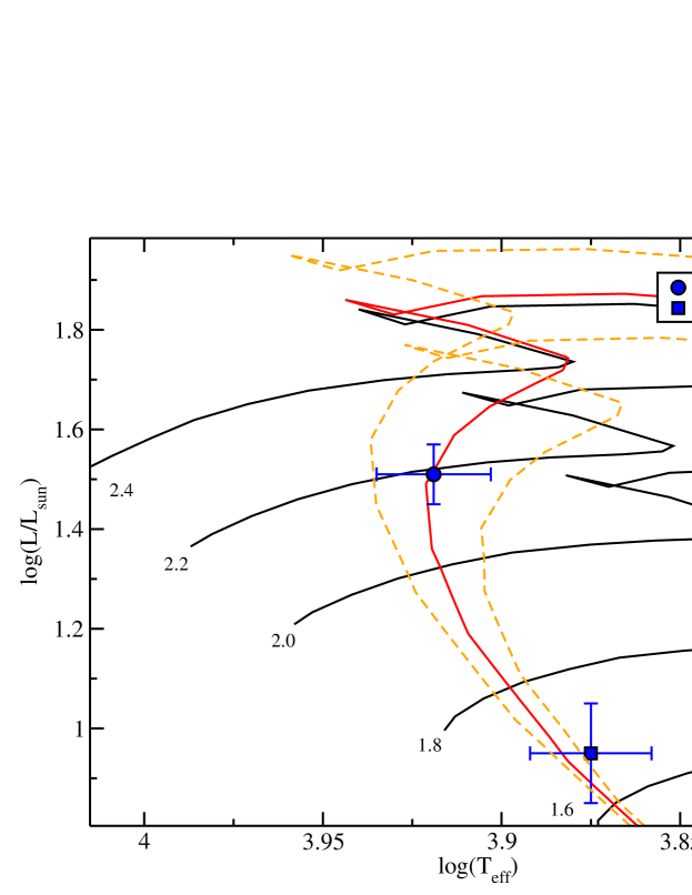
Figure 4: The positions of HD 98088 A and B on the H-R diagram. Evolutionary tracks (black) are labelled in units of solar masses, and isochrones correspond to the age of the system ($8.81\pm 0.06$ log yr). Evolutionary tracks and isochrones are from Schaller et al. (1992) for standard mass loss and $Z=0.02$.

A few additional useful parameters can be calculated, and a few consistency checks can be made between our H-R diagram parameters and our dynamic parameters from the radial velocity curve. The mass ratio from the H-R diagram $M_{\rm A}/M_{\rm B}=1.31\pm 0.08$ agrees well with the more precise dynamic value $M_{\rm A}/M_{\rm B}=1.374\pm 0.008$. Combining the dynamic $M_{\rm A}\sin^{3}i$ with the H-R diagram $M_{\rm A}$ we derive the inclination of the orbital axis with respect to the line of sight $i_{\rm orb}=69\pm 2\degr$. Using the secondary’s mass we find the consistent value $i_{\rm orb}=67\pm 2\degr$. Then the semi-major axis of the primary’s orbit can be calculated, using the dynamic $a_{\rm A}\sin i$, yielding $a_{\rm A}=9.03\pm 0.10$ $R_{\odot}$. Similarly, for the secondary $a_{\rm B}=12.40\pm 0.15$ $R_{\odot}$. We also calculate the inclination of the rotational axis of the primary, using the rotational period from the magnetic analysis and $v\sin i$ from the abundance analysis, and find $i_{\rm rot,A}=68^{+22}_{-17}\degr$. While this is rather uncertain, it is consistent with the orbital inclination, which one would expect for a tidally locked system. We can also calculate $\log\,{g}$ based on the star’s H-R diagram masses and radii, finding $\log\,{g}$ $=3.90\pm 0.09$ for the primary and $\log\,{g}$ $=4.16\pm 0.12$ for the secondary. These are consistent with the values from the SED, but significantly more precise.

We can also compare our values to the detailed work of Carrier et al. (2002), and we find our physical parameters are fully consistent with theirs. Our orbital periods and inclinations are consistent, as are our $T_{\rm eff}$, $\log\,{g}$, luminosities, masses and radii.

6 Chemical Abundances

A detailed abundance analysis was performed for both HD 98088 A and B, using the disentangled spectra. Two independent procedures were adopted, and independent analyses were performed by two of us. One analysis (performed by K.L.) employed the LTE spectrum synthesis code Synth3 (Kochukhov, 2007) coupled to the IDL visualisation script BinMag. The other analysis (performed by C.P.F.) employed a modified version of the Zeeman spectrum synthesis code (Landstreet, 1988; Wade et al., 2001) which solves the polarized radiative transfer equations, again assuming LTE. Optimizations to the code for negligible magnetic fields were included, and a Levenberg-Marquardt $\chi^{2}$ minimisation routine was used to aid in fitting the observed spectrum (Folsom et al., 2012).

In both cases, atomic data was extracted from the Vienna Atomic Line Database (VALD) (Kupka et al., 1999), using an ‘extract stellar’ request, with temperatures tailored to the components of HD 98088. The model atmospheres used in the abundance analysis were calculated using the LLModels code (Shulyak et al., 2004), which produces LTE model atmospheres with detailed line blanketing. Prior to abundance analysis, the average disentangled spectra of the primary and secondary were corrected for the continuum dilution by the other component (see e.g. Folsom et al., 2008) using the theoretical, wavelength dependent light ratio predicted by the adopted LLModels atmospheres.

The Synth3 analysis involved directly fitting synthetic spectra to the deconvolved spectra of both components of HD 98088. The fitting was performed independently on a number of small spectral windows. For the primary, 20 spectral windows were used with typical lengths of 100 Å (ranging from 50 to 150 Å long), running from 4500 to 6500 Å, excluding Balmer lines. For the secondary, 13 windows were used typically with 150 Å lengths, again running from 4500 to 6500 Å excluding Balmer lines. The fitting was performed by manually adjusting input chemical abundances, $v\sin i$, and microturbulence, then evaluating the fit of the synthetic spectrum to the observation with the BinMag visualisation tool. The best fit values from the individual windows were averaged to produce the final best values, and the uncertainties on the final best values were taken to be the standard deviation of the values from individual windows. For elements with abundances derived only in three or fewer windows, the uncertainty was taken to include the line-to-line scatter as well as the range of abundances produced by varying $T_{\rm eff}$ and $\log\,{g}$ by $1\sigma$. The final best fit values are reported in Table 4.

The Zeeman analysis proceeded by fitting the spectra of both stars independently for chemical abundances, as well as $v\sin i$  and microturbulence. Fitting was performed for 6 independent spectral regions, between 200 and 400 Å long, covering a spectral range from 4900 to 6500 Å. The final best fit values adopted are averages of the results over all 6 windows, with the adopted uncertainty as the standard deviation of those results. For elements with less than four lines available, the the uncertainty was estimated by eye instead, including potential normalisation errors, blended lines, and the scatter between lines. The final averaged best fit values and uncertainties are presented in Table 4. The best fit chemical abundances are plotted, relative to the solar values of Asplund et al. (2009), in Fig. 5 for both components of HD 98088.

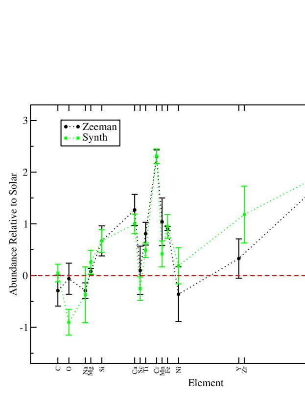
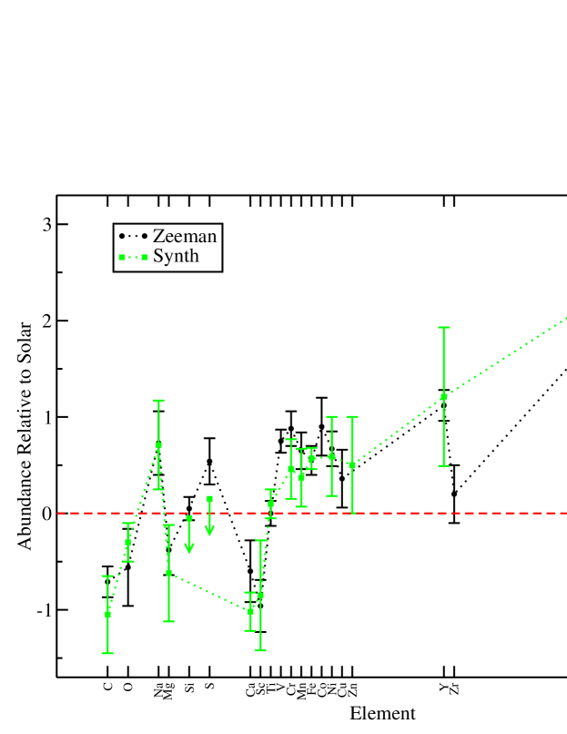
Figure 5: Abundances relative to solar for HD 98088 A (top frame) and HD 98088 B (bottom frame), averaged over all spectral windows modelled. The results from both the analysis with Zeeman (circles, black) and Synth3 (squares, green) are presented. Solar abundances are taken from Asplund et al. (2009). Arrows represent upper limits only.

Table 4: Summary of abundances, $v\sin i$, and microturbulence ($\xi$) for HD 98088 A and B, for both the analysis with Synth3 and Zeeman. Chemical abundance are in units of $\log(N_{X}/N_{tot})$. For the Synth3 results, abundances fit manually with lines from three or fewer spectral regions are marked with an asterisk (*). For the Zeeman results, abundances fit with three or less useful lines are marked with an double-asterisk (**). Solar abundances are from Asplund et al. (2009).

	HD 98088 A	HD 98088 B	HD 98088 A	HD 98088 B	Solar
	Synth3	Synth3	Zeeman	Zeeman
$v\sin i$ (km s-1)	$22.0\pm 1.5$	$18.0\pm 2.0$	$24.4\pm 0.8$	$20.6\pm 0.8$
$\xi$ (km s-1)	$1.0\pm 0.5$	$1.5\pm 0.5$	$2.0$	$1.9\pm 0.2$
C	-3.52 $\pm$ 0.17*	-4.62 $\pm$ 0.40*	-3.86$\pm$0.30**	$-4.28\pm 0.16$	-3.57
O	-4.21 $\pm$ 0.25*	-3.61 $\pm$ 0.20*	-3.38$\pm$0.30**	$-3.87\pm 0.40$**	-3.31
Na	-6.13 $\pm$ 0.54*	-5.05 $\pm$ 0.46	-6.05$\pm$0.15**	$-5.03\pm 0.33$**	-5.76
Mg	-4.14 $\pm$ 0.23	-5.02 $\pm$ 0.50*	-4.32$\pm$0.06	$-4.78\pm 0.26$	-4.40
Si	-3.82 $\pm$ 0.22	$\leq$-4.54	-3.82$\pm$0.29	$-4.44\pm 0.12$	-4.49
S		$\leq$-4.73		$-4.34\pm 0.24$	-4.88
Ca	-4.66 $\pm$ 0.19	-6.68 $\pm$ 0.20	-4.39$\pm$0.30	$-6.26\pm 0.32$	-5.66
Sc	-9.10 $\pm$ 0.23	-9.70 $\pm$ 0.57	-8.75$\pm$0.47	$-9.81\pm 0.27$	-8.85
Ti	-6.56 $\pm$ 0.14	-6.95 $\pm$ 0.15	-6.24$\pm$0.22	$-7.05\pm 0.13$	-7.05
V				$-7.32\pm 0.12$	-8.07
Cr	-4.05 $\pm$ 0.14	-5.90 $\pm$ 0.31	-4.06$\pm$0.13	$-5.48\pm 0.18$	-6.36
Mn	-6.15 $\pm$ 0.25*	-6.20 $\pm$ 0.30*	-5.53$\pm$0.46	$-5.92\pm 0.19$	-6.57
Fe	-3.55 $\pm$ 0.23	-3.93 $\pm$ 0.11	-3.59$\pm$0.04	$-3.95\pm 0.15$	-4.50
Co				$-6.11\pm 0.30$**	-7.01
Ni	-5.59 $\pm$ 0.35	-5.19 $\pm$ 0.41	-6.14$\pm$0.53	$-5.11\pm 0.18$	-5.78
Cu				$-7.45\pm 0.30$**	-7.81
Zn		-6.94 $\pm$ 0.50*			-7.44
Y		-8.58 $\pm$ 0.72	-9.46$\pm$0.38	$-8.67\pm 0.16$**	-9.79
Zr	-8.24 $\pm$ 0.55*			$-9.22\pm 0.30$	-9.42
Ba	-7.76 $\pm$ 0.10	-7.46 $\pm$ 0.37	-7.83$\pm$0.15	$-7.74\pm 0.35$**	-9.82
La		-9.37 $\pm$ 0.40*		$-9.26\pm 0.16$	-10.90
Ce			-9.03$\pm$0.24	$-8.95\pm 0.15$	-10.42
Pr			-9.56$\pm$0.39	$-9.63\pm 0.18$	-11.28
Nd	-9.40 $\pm$ 0.84		-9.34$\pm$0.20	$-9.12\pm 0.28$	-10.58
Sm			-8.85$\pm$0.17	$-9.13\pm 0.14$	-11.04
Eu			-8.84$\pm$0.31**	$-9.38\pm 0.30$**	-11.48

6.1 Abundances of HD 98088 A

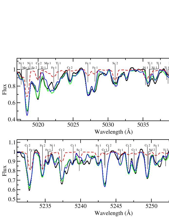
Figure 6: Typical fits to the spectrum of HD 98088 A for both the Zeeman and Synth3 results. Points represent the observation, the lighter grey (green) line is the Zeeman, and the darker grey (blue) line is the Synth3 best fit spectrum. The dashed line is a synthetic spectrum with solar abundances. Elements which are major contributors to each line have been labelled.

The best fit synthetic spectra from both the Zeeman and the Synth3 analyses generally reproduce the observed disentangled spectrum well. Samples of typical fits to the observation for both analyses of HD 98088 A are presented in Fig. 6. Small differences between both synthetic spectra and the observation do exist. This is likely due to chemical stratification, which is common in Ap stars, or to blending with unknown rare-earth lines, which can also occur in Ap stars at these temperatures.

HD 98088 A clearly shows typical Ap peculiarities, with strong overabundance of Si, Ca, Ti, Mn, Fe, and Ni, a dramatic overabundance of Cr, and very strong overabundances of Ba, Ce, Pr, Nd, Sm and Eu. Ni and Sc have nearly solar abundances, as do C, O, Na, and Mg.

In order to approximate the desaturation effect of the magnetic field of HD 98088 A in our spectra, a microturbulence of 2 km s^-1 was assumed for the Zeeman analysis and a value of 1 km s^-1 was used for the Synth3 analysis. While the difference in assumed microturbulence was a consequence of the independent analyses, it serves to illustrate the minor impact that small variations in microturbulence have on our results. There are a half-dozen careful analyses of sharp lined Ap stars published in the literature (e.g. Ryabchikova et al., 1997; Kochukhov et al., 2006, from Ryabchikova private communication), all of which find microturbulence consistent with zero. Thus, while the typical microturbulence in an Ap star is unknown, it is likely small. The use of microturbulence for HD 98088 A is simply to approximate line broadening due to the magnetic field, thereby reducing the computation time for spectra dramatically. Replacing the microturbulence with a dipole magnetic field like that determined in Sect. 7 would modify most of our abundances by 0.1-0.2 dex, which is generally within our uncertainties.

The abundance of HD 98088 A derived from the two analyses agree very well. The abundances all agree within $1\sigma$, except for Ti and Mn at $1.2\sigma$ and O at $2\sigma$. Both O abundances are based on one weak, heavily blended triplet of lines (6156-6158 Å), thus an additional systematic effect may be present, or the uncertainties may be underestimated. The $v\sin i$ values agree at $1.4\sigma$. No systematic differences between the results are found.

An attempt was made to determine a spectroscopic $T_{\rm eff}$ and $\log\,{g}$ by fitting metal lines of varying excitation potentials and ionisation states using the Zeeman program and the method described by Folsom et al. (2012). This attempt was unsuccessful. While we found $\log\,{g}$ $=4.1\pm 0.2$ which appears to be accurate, we also found $T_{\rm eff}$ $=9000\pm 200$ K which is clearly inconsistent with the observed SED. A likely cause of this discrepancy is chemical stratification in HD 98088 A, which could cause lines formed deeper in the stellar atmosphere to be anomalously strong, thereby producing an incorrect $T_{\rm eff}$ estimate when metallic lines are used.

The presence of chemical stratification in HD 98088 A was investigated using the Zeeman spectrum synthesis program. While stratification is not the focus of this study, these results could prove instructive for future studies, and they help explain the initial inaccurate spectroscopic $T_{\rm eff}$. Stratification was modelled with a simple step function, consisting of one abundance deeper in the atmosphere, another abundance higher in the atmosphere, and an optical depth for the transition. In this pilot study Fe stratification was investigated, while other elements were assumed to have homogeneous abundances. The optical depth scale used was the optical depth (due to continuous opacity) at the middle of the wavelength region modelled. The Fe stratification parameters were added to the $\chi^{2}$ minimisation routine, and they as well as all other abundances and $v\sin i$ were fit simultaneously, while the atmospheric parameters were held fixed at the values in Table 3. The fitting was performed for the 4900-5500 Å, 5500-5700 Å, and 6100-6500 Å regions independently. The resulting fits provide a clear improvement over a homogeneous model, both by visual inspection and by $\chi^{2}$. Averaging over the three windows, and taking the range of values as the uncertainty, the Fe abundance higher in the atmosphere (lower optical depth) is ${\rm Fe}_{upper}=-4.5\pm 0.2$ dex, the Fe abundance deeper in the atmosphere is ${\rm Fe}_{lower}=-2.2\pm 0.3$ dex, and the transition occurs at $\log\tau=-0.3\pm 0.2$. While this represents strong Fe stratification, it is similar to what is seen in other Ap stars of similar $T_{\rm eff}$ (e.g. Ryabchikova et al., 2002, 2005; Kochukhov et al., 2009).

We then attempted to determine a spectroscopic $T_{\rm eff}$ simultaneously with Fe stratification (relying principally on the ionisation balance for $T_{\rm eff}$). This was done by using the $\chi^{2}$ minimisation routine to fit $T_{\rm eff}$, Fe stratification, $v\sin i$, and other chemical abundances simultaneously, again using the 4900-5500 Å, 5500-5700 Å, and 6100-6500 Å spectral regions. We find $T_{\rm eff}$ $=8500\pm 300$ K, ${\rm Fe}_{upper}=-4.0\pm 0.2$ dex, ${\rm Fe}_{lower}=-2.2\pm 0.4$ dex, and $\log\tau=-0.5\pm 0.3$. This $T_{\rm eff}$ is consistent with the SED of HD 98088. The stratification result is is also consistent with the previous values, though the small difference in ${\rm Fe}_{upper}$ suggests it may be sensitive to the exact $T_{\rm eff}$ used. As a note of caution, since only the stratification of Fe was modelled here, stratification of other elements could be influencing the derived $T_{\rm eff}$ potentially making it slightly inaccurate. However, this model does succeed in reconciling the spectroscopic and spectrophotometric observations.

6.2 Abundances of HD 98088 B

We achieve good fits to the observed spectrum of HD 98088 B for both the Synth3 and Zeeman analyses. Typical fits from both analyses of HD 98088 B are presented in Fig. 7. Both sets of best fit abundances for HD 98088 B are reported in Table 4, and plotted relative to solar in Fig. 5.

The abundances we find reveal that HD 98088 B is a clear Am star. We find strong overabundances of Cr, Mn, Fe, Co, Ni, and Y, and very strong overabundances of Ba, La, Cr, Pr, Nd, Sm and Eu. Sc and Ca are strongly underabundant, C appears to be underabundant, and O and Mg are marginally underabundant. This pattern of abundances, with overabundant Fe-peak elements and rare-earths, and underabundant Ca and Sc is characteristic of Am stars. We also find a small microturbulence of $\approx 2$ km s^-1.

In the Zeeman analysis, microturbulence was determined by including it as a free parameter in the $\chi^{2}$ analysis and fit simultaneously with chemical abundances. In the Synth3 analysis, microturbulence was determined by fitting the synthetic spectrum to the observation by eye, together with chemical abundances. Microturbulence is often elevated in Am stars (typically 2 to 4 km s^-1, e.g. Landstreet et al., 2009), and thus can have a significant impact on the abundance analysis of these stars.

The results for the two abundance analyses agree very well. The chemical abundances, $v\sin i$, and microturbulence all agree within $1\sigma$, except for Ca and Cr which agree at $1.1\sigma$ and $1.2\sigma$ respectively. This confirms the accuracy of our methodology. Our uncertainties, if anything, may be slightly overestimated, since statistically one would expect a few of our results to deviate by more than $1\sigma$.

We attempted to determine a spectroscopic $T_{\rm eff}$ for HD 98088 B using fits to metallic lines, similarly to HD 98088 A. This was done using Zeeman and independent fits for all 6 windows used for the abundance analysis. The produced a value of $T_{\rm eff}$ $=8000\pm 300$ K, which is consistent with the result from the SED at the $1.2\sigma$ level. We prefer the SED value, since the spectroscopic $T_{\rm eff}$ could be influenced by any small systematic errors in the disentangled spectrum, or by inaccurate or missing atomic data, particularly for the strongly overabundant rare-earth elements.

This is the first report of chemical peculiarities in HD 98088 B, and a very rare case of a binary system with an Ap primary and an Am secondary. However, the appearance of Am peculiarities in HD 98088 B may reflect the generally higher incidence of Am peculiarities in low $v\sin i$ stars (Abt & Morrell, 1995), and in binary systems (e.g. Carquillat & Prieur, 2007).

Figure 7: Typical fits to the spectrum of HD 98088 B for both the Zeeman and Synth3 results. Points represent the observation, the lighter grey (green) line is the Zeeman, and the darker grey (blue) line is the Synth3 best fit spectrum. The dashed line is a synthetic spectrum with solar abundances. Elements which are major contributors to each line have been labelled.

7 Magnetic fields of the components

The magnetic fields in the photospheres of HD 98088 A and B were studied using the circular and linear polarisation within the LSD profiles, produced as a consequence of the longitudinal and transverse Zeeman effect.

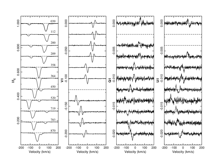
Figure 8: LSD Stokes $IVQU$ profiles extracted from the observations of HD 98088. The weaker line of the secondary is visible in the leftmost frame. Polarisation signatures are observed at the position of the mean line of the primary, and follow the orbital motion of that line. No polarisation is observed at the position of the mean line of the secondary. Phases ($\times 1000$) are labelled in the leftmost frame.

Fig. 8 illustrates the extracted Stokes $I$, $V$, $Q$ and $U$ LSD profiles, ordered according to orbital phase. In the leftmost frame, the mean Stokes $I$ profiles of both the primary and secondary stars are visible, and exhibit systematic displacement as a consequence of their orbital motion. The relative weakness of the secondary’s mean line is notable. In the remaining 3 panels, it is clear that Stokes $V$, $Q$ and $U$ Zeeman signatures are detected only at the position of the mean line of the primary star, indicating (at least at first glance) that the secondary is non-magnetic. Indeed, evaluating the detection probability according to the criteria introduced by Donati et al. (1997) indicates that significant Stokes $V$ signal is detected in the mean line of the primary star at all phases, whereas no significant signal is ever detected in the mean line of the secondary. Finally, we point out the excellent phasing of the LSD profiles according to the orbital period. Although the data span more than 180 orbits of the system, there is excellent fidelity of the detailed profile shapes and positions inferred to correspond to similar phases, and acquired both close together or far apart in time (e.g. phases 0.200/0.209 and 0.358/364). This is the most visually striking evidence for precise synchronization of the orbital period and the rotational period of the magnetic primary star.

To quantify the magnetic properties of the two stars, we measured the longitudinal magnetic field $B_{\ell}$ of both components from the LSD profiles using the first-moment method of Rees & Semel (1979). We integrated the $I/I_{\rm c}$ and $V/I_{\rm c}$ profiles about their centres-of-gravity $v_{\rm 0}$ in velocity $v$, in the manner implemented by Donati et al. (1997) and corrected by Wade et al. (2000):

$$B_{\ell}=-2.14\times 10^{11}\ \frac{{\displaystyle\int(v-v_{\rm 0})V(v)\ dv}}{\displaystyle{\lambda zc\ \int[1-I(v)]\ dv}}.$$ (1)

In Eq. 1 $V(v)$ and $I(v)$ are the $V/I_{\rm c}$ and $I/I_{\rm c}$ LSD profiles, respectively. The wavelength $\lambda$ is expressed in nm and the longitudinal field $B_{\ell}$ is in gauss. The wavelength and Landé factor $z$ correspond to the mean values employed in computing the LSD profiles, reported in Sect. 2.

For the primary, the velocity integration limits for the evaluation of Eq. 1 were selected manually to include the entire observed Stokes $V$ profile. In the case of the secondary, the limits were chosen to include the entire Stokes $I$ profile. The centre-of-gravity for each component was also calculated using these integration limits. Table 5 summarises the longitudinal magnetic field measurements for each date for which Stokes $V$ observations were obtained. At phases at which the profiles of the primary and secondary star were blended, we measured only the longitudinal field of the primary star by assuming that the secondary made no contribution to the Stokes $V$ profile, and adjusting the denominator of Eq. 1 by subtracting the average equivalent width of the secondary’s LSD profile. Standard uncertainty propagation was used to determine the $1{\sigma}$ error bars on the longitudinal magnetic field measurements. Uncertainties range from $15$ to $35$ G for the primary and from $78$ to $280$ G for the secondary component. A significant longitudinal magnetic field is detected in the primary component at all phases. On the other hand, no significant magnetic field is ever detected in the secondary component.

We point out that the value of the longitudinal field of a component of an SB2 system inferred using Eq. 1 is unaffected by the continuum of the companion. This is because it is the continuum normalised Stokes $I$ and $V$ parameters ($I/I_{\rm c}$ and $V/I_{\rm c}$, respectively) that appear in the denominator and numerator of Eq. 1. Nevertheless, the inferred uncertainty, derived from photon-noise error bars propagated through the LSD procedure, is larger than that for the single-star case.

From these basic magnetic measurements, we conclude that the primary component of HD 98088 hosts a strong magnetic field with a peak disc-averaged longitudinal component of about 1100 G, whereas the secondary shows no detectable magnetic field.

7.1 Rotational period and magnetic geometry of the primary star

The Lomb-Scargle periodogram of the longitudinal field measurements of the primary star displays a clear excess of power between 5.6 and 6.0 d, with many possible solutions in this range. The peak closest to the orbital period corresponds to a variability period of 5.90451 d, but with rather large uncertainties ($\sim\pm 0.0015$ d). If we combine our new longitudinal field measurements with those reported by Babcock (1958), this yields a period of $5.90510\pm 0.00003$ d. This rotational period is in excellent agreement with the orbital period ($5.9051102\pm 0.0000023$; Table 1). Given this correspondence and the better precision of the orbital period, hereinafter we assume perfect synchronization of the system and adopt the orbital period as the rotational period of both the primary and secondary stars.

The phased longitudinal field measurements are shown along with those of Babcock (1958) in Fig. 9. The significant improvement in precision of the MuSiCoS data relative to Babcock’s measurements is evident. Although the historical measurements are noisy, it appears that the new $B_{\ell}$ curve may be shifted to slightly ($\sim 100-150$ G) higher values than the previous measurements. If real, we attribute this shift to differences in the modelling and analysis methods employed. Such a difference is not surprising, since the older measurements were based on (somewhat non-linear) photographic data, with line centres estimated by eye. Babcock’s observations were made blueward of H$\beta$, while our observations are predominately to the red of that line, thus the two datasets are affected by limb darkening somewhat differently, which could also partly explain the discrepancy. Our new measurements show clear and systematic departures from a pure sinusoidal variation. Whereas first-order and second-order harmonic expansions fit phase variation of the new data rather poorly (reduced $\chi^{2}$ of 16.1 and 18.6, respectively), a third-order expansion achieves an excellent fit (reduced $\chi^{2}$ of 0.6). While these departures from a sinusoidal variation may diagnose non-dipolar characteristics of the stellar magnetic field, it is more likely that they reflect the non-uniform distributions of chemical elements whose lines were used to measure the field.

To determine the magnetic geometry of the primary, we took advantage of the Stokes $Q$ and $U$ LSD profiles to measure the net linear polarization (NLP), integrated across the LSD profiles (Wade et al., 2000; Silvester et al., 2012). These data are reported in Table 5 and are compared to the broadband linear polarization (BBLP) measurements of HD 98088 reported by Leroy et al. (1995). in Fig. 10. As described by e.g. Silvester et al. (2012), while NLP and BBLP result from the same physical mechanism, the methods of measurements are sufficiently different that their intercomparison requires that one data set be arbitrarily shifted and scaled relative to the other. The NLP values reported in Table 5 and illustrated in Fig. 10 include this scaling and shifting. The BBLP and NLP phase variations are generally compatible, although some differences in detail are certainly present. These results are consistent with the general results reported by Wade et al. (2000) and Silvester et al. (2012).

In combination with the longitudinal field, the NLP/BBLP measurements provide an unambiguous estimate of the rotational axis inclination $i$, magnetic obliquity $\beta$ and polar field strength $B_{\rm d}$, under the assumption of a pure dipolar surface magnetic field configuration (Leroy et al., 1995). A first-order harmonic fit to Babcock’s data yields $B_{\ell,{\rm max}}=1050\pm 175$ G and $B_{\ell,{\rm min}}=-1280\pm 175$ G, giving $r=B_{\ell,{\rm max}}/B_{\ell,{\rm min}}=-0.82\pm 0.22$. An analogous fit to the MuSiCoS measurements yields $B_{\ell,{\rm max}}=1185\pm 65$ G and $B_{\ell,{\rm min}}=-1000\pm 65$ G, for $r=-0.84\pm 0.09$. The broadband linear polarization measurements of Leroy et al. give $s=-0.065\pm 0.13$, where $s$ is a (unitless) parameter describing the harmonic content of the NLP/BBLP phase variation, defined according to Leroy et al. (1995). For the NLP variation, this value is $+0.005\pm 0.20$. The combined values of $r$ and $s$ yield unique values for the angles $i$ and $\beta$.

Using this method Leroy et al. (1996) reported $i=85\pm 5\degr$ and $\beta=80\pm 5\degr$ for HD 98088 A. For the combination of BBLP + Babcock, we find $i=75\pm 15\degr$ and $\beta=73\degr\pm 3\degr$. For BBLP + MuSiCoS $B_{\ell}$, we find $i=77\pm 10\degr$ and $\beta=73\degr\pm 3\degr$. Finally, for NLP + MuSiCoS $B_{\ell}$, we find $i=77\pm 10\degr$ and $\beta=76\degr\pm 5\degr$. All of these values are in good mutual agreement, indicating that the systematic differences between the various data sets are not a major source of error. We also note that the derived values of the inclination $i$ are formally consistent with the orbital inclination determined from the masses ($68\pm 3\degr$).

If we adopt the orbital inclination as the inclination of the rotation axis of the primary, along with $\beta=75\pm 5\degr$, we derive the surface polar strength of the primary’s magnetic dipole to be $3850\pm 450$ G using the MuSiCoS measurements.

7.2 Upper limit on magnetic field of the secondary star

No magnetic signature is detected in the mean line of the secondary, nor is the longitudinal magnetic field detected with significance. However, we can estimate an upper limit on the dipole component of the secondary. Assuming the secondary’s rotation is synchronized with the orbit, i.e. with rotational period equal to $P_{\rm orb}$ and rotation axis inclination $i=68\degr$, the median longitudinal field error bar of 160 G translates into a $3\sigma$ upper limit on the surface dipole of roughly 1550 G.

Table 5: Magnetic measurements obtained from MuSiCoS spectra. All phases are computed from the orbital ephemeris. HJD is from the Stokes V observation. Typical range of phase corresponding to a single Stokes $VQU$ sequence is approximately $0.01\times P_{\rm orb}$.

Date	${\bar{\rm HJD}}$	Orbital	$B_{\ell}$ (G)		NLP
	(2,450,000+)	Phase	Primary	Secondary	$Q/I$ (%)	$U/I$ (%)
18 Jan 99	1197.617	0.358	$1048\pm 15$		$0.015\pm 0.004$	$0.048\pm 0.004$
23 Jan 99	1202.590	0.200	$384\pm 33$	$51\pm 166$	$0.027\pm 0.007$
24 Jan 99	1203.555	0.364	$1062\pm 19$		$0.007\pm 0.005$	$0.043\pm 0.005$
05 Mar 00	1609.524	0.112	$-370\pm 24$	$-210\pm 135$
07 Mar 00	1611.519	0.450			$0.004\pm 0.005$	$0.067\pm 0.005$
05 Dec 01	2249.685	0.520	$1167\pm 27$	$-195\pm 193$	$0.008\pm 0.008$	$0.086\pm 0.009$
07 Dec 01	2251.751	0.870	$-916\pm 19$	$53\pm 78$	$-0.035\pm 0.004$	$0.039\pm 0.005$
08 Dec 01	2252.748	0.039	$-762\pm 28$	$-92\pm 133$	$0.041\pm 0.006$	$0.062\pm 0.006$
09 Dec 01	2253.750	0.209	$435\pm 21$	$226\pm 112$	$0.023\pm 0.006$	$0.102\pm 0.006$
12 Dec 01	2256.762	0.719	$-291\pm 35$	$423\pm 280$	$-0.034\pm 0.005$	$0.094\pm 0.006$
05 Jan 02	2280.759	0.783	$-674\pm 30$	$-159\pm 156$	$-0.036\pm 0.006$	$0.070\pm 0.007$

Figure 9: Phased longitudinal magnetic field measurements of HD 98088 A. Filled squares - MuSiCoS measurements. Open triangles - Measurements reported by Babcock (1958). The vertical dashed lines indicate the approximate quadrature phases of the radial velocities.

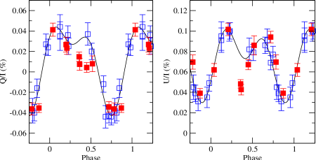
Figure 10: Net linear polarisation of HD 98088 A, compared to the broadband linear polarization measurements of Leroy et al. (1995). As discussed by e.g. Silvester et al. (2012), the MuSiCoS measurements have been arbitrarily shifted and scaled to reproduce as closely as possible the broadband variations.

8 Discussion and Conclusions

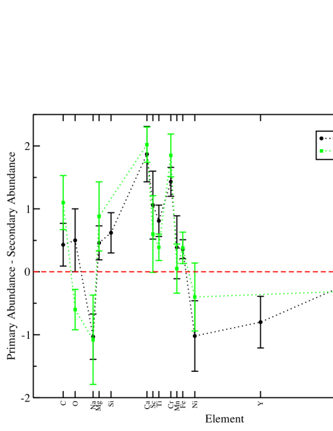
Figure 11: Differential comparison of the chemical abundances found for the primary and secondary of HD 98088. Values from both the Synth3 (squares, green) analysis and the Zeeman (circles, black) analysis are presented.

Figure 12: Schematic of the orbit of HD 98088 A (circle with arrow) from the reference frame of HD 98088 B (filled circle). A dipole magnetic field for HD 98088 A is indicated with an arrow, assuming the dipole is aligned with the secondary at periastron. The dotted line represents the line towards the observer. The stellar radii and orbital separation are approximately to scale. Phases where the observed longitudinal magnetic field ($B_{l}$) is a maximum, minimum, and zero are shown, as are phases where the stars are aligned along the line of sight. Note that the phases where the radial velocities of the components are equal are shifted slightly from the phase where the stars are aligned along the line of sight (by +0.01 and -0.03 in phase), due to the eccentricity of the orbit.

We find strong chemical peculiarities in HD 98088 A that are characteristic of a cool Ap star. In HD 98088 B we also find strong chemical peculiarities indicative of an Am star. We also find evidence of strong Fe stratification in the atmosphere of the primary. The introduction of stratification was necessary to reconcile the spectroscopic and spectrophotometric temperatures of HD 98088 A. While Am stars are often found in close binary systems, HD 98088 represents one of very few close binary systems with an Ap component.

Both components of HD 98088 have similar masses, $T_{\rm eff}$, $\log\,{g}$, and $v\sin i$, yet the components display very different chemical peculiarities. Fig. 11 illustrates the difference in the derived abundances between the primary and the secondary. The components of HD 98088 are likely coeval, but a qualitative difference is the presence of a strong magnetic field in the primary. This suggests that the observed differences in chemical abundances are due to the impact of the magnetic field on atomic diffusion in the atmosphere of the primary (e.g. Michaud et al., 1981).

We find a strong, predominately dipolar, magnetic field in HD 98088 A, with a longitudinal strength varying from +1170 to -920 G. Conversely, we find no magnetic field in the secondary with longitudinal field error bars down to 112 G, and a typical error bar of 160 G. We also find no signal from the secondary in linear polarisation, while the magnetic field of the primary is detected in linear polarisation at all phases. The predominately dipolar nature of the magnetic field in the primary is shown by the longitudinal field and net linear polarisation curves, and by the simple structure of the $V$, $Q$, and $U$ LSD profiles.

It is not clear why the primary has a strong magnetic field and the secondary has no magnetic field when the two stars have similar masses and temperatures, and are apparently coeval with identical ages. Indeed, the origin of the magnetic fields in Ap stars is one of the enduring mysteries that these stars present.

We derived improved orbital parameters for the HD 98088 system, finding a period of $5.9051102\pm 0.0000023$ days. We also derive a rotational period for HD 98088 A of $5.90510\pm 0.00003$ days, which is consistent with the orbital period. This provides strong evidence that the system is tidally locked, with the rotational and orbital periods synchronised. We derive an inclination of the orbital axis of the system of $i_{\rm orb}=69\pm 2\degr$, which is consistent with the inclination of the rotational axis of the primary based on its rotational period, $v\sin i$, and radius, as well as the inclination derived from the linear polarisation under the assumption of a dipole magnetic field. However, the system has a modest but significant eccentricity of $0.1840\pm 0.0025$, which is clearly visible in the radial velocity curve presented in Fig. 1. Thus while the system is synchronised, the orbits apparently have not had the time to circularise.

Hut (1981) showed that, in binary systems where orbital angular momentum dominates over rotational angular momentum, tidal interactions cause the orbital and rotational axes to become parallel, and the orbital and rotational periods to become synchronised, much more quickly than they circularise the orbits of the system. Using Eq. 22 of Hut (1981) (and assuming an approximate radius of gyration of 0.2, following Stȩpień 2000), the ratio of orbital to rotational angular momentum is $\sim$150 for the primary, and $\sim$500 for the secondary. This suggests (Hut, 1981, Eq. 33) that circularisation of the orbits would be slower by a factor of $\sim$100 than the synchronisation of orbital and rotational periods. Thus it is certainly possible for HD 98088 to be rotationally synchronised but still have elliptical orbits. However, we find an age for the system of $8.81\pm 0.06$ $\log{\rm yr}$, which suggests that tidal interactions would have to be very inefficient for the system to still have some ellipticity.

Modelling the magnetic field of HD 98088 A as a dipole, we find a dipole strength of $3850\pm 450$ G and an obliquity angle of $\beta=75\pm 5\degr$. The longitudinal magnetic field reaches an extremum at very near the quadrature orbital phases (where the radial velocities of both components are near zero, see Figs. 1 and 9). Thus the magnetic dipole is close to being aligned along the axis between the two stars, with the positive magnetic pole always pointing near the secondary, as illustrated in Fig. 12. This analysis does not account for the influence of abundance spots on the $B_{\ell}$ curve, and if this effect were accounted for (with a self consistent modelling procedure, such as magnetic Doppler imaging) the alignment could be exact. This is likely significant, though the interpretation of this observation is not immediately obvious. It could be that the tidal interaction between the components somehow influenced the stable magnetic field geometry of the primary. For example if the magnetic field had a fossil origin as in the models of Braithwaite & Nordlund (2006), then tidal effects could affect the evolution of the magnetic field towards its stable configuration. However, magnetic fields in Ap stars appear to originate very early in a star’s lifetime (Wade et al., 2005, in a few Myr), and the orbital parameters may have changed since then. One could speculate that tidal interactions over the intervening years could have caused the field to evolve into its present configuration. Alternately, if the magnetic field perturbed the structure of the primary sufficiently to produce a small over-density at the magnetic poles, the system could settle into its current configuration through tidal effects.

HD 98088 represents a very rare case of a magnetic Ap star in a tidally locked binary system with an Am star. The magnetic field in the Ap star is predominately dipolar, with the positive pole always pointing towards the secondary. Further studies could help clarify the interpretation of this result. Magnetic Doppler imaging of HD 98088 A would be particularly valuable, as this would provide a more detailed model of the magnetic field, as well as a map of chemical inhomogeneities across the surface of the star. These would be particularly interesting in the context of tidal interactions with the secondary. HD 98088 is an ideal target for the Binarity and Magnetic Interactions in Stars (BinaMIcS) project, and further observations and analysis are planned by the collaboration.

References

- Abt (1953) Abt H. A., 1953, PASP, 65, 274
- Abt et al. (1968) Abt H. A., Conti P. S., Deutsch A. J., Wallerstein G., 1968, ApJ, 153, 177
- Abt & Morrell (1995) Abt H. A., Morrell N. I., 1995, ApJS, 99, 135
- Adelman et al. (1989) Adelman S. J., Pyper D. M., Shore S. N., White R. E., Warren, Jr. W. H., 1989, A&AS, 81, 221
- Alecian et al. (2008) Alecian E. et al., 2008, MNRAS, 385, 391
- Asplund et al. (2009) Asplund M., Grevesse N., Sauval A. J., Scott P., 2009, ARA&A, 47, 481
- Aurière et al. (2007) Aurière M. et al., 2007, A&A, 475, 1053
- Babcock (1958) Babcock H. W., 1958, ApJS, 3, 141
- Balona (1994) Balona L. A., 1994, MNRAS, 268, 119
- Baudrand & Bohm (1992) Baudrand J., Bohm T., 1992, A&A, 259, 711
- Bonsack (1976) Bonsack W. K., 1976, ApJ, 209, 160
- Braithwaite & Nordlund (2006) Braithwaite J., Nordlund Å., 2006, A&A, 450, 1077
- Carquillat & Prieur (2007) Carquillat J.-M., Prieur J.-L., 2007, MNRAS, 380, 1064
- Carrier et al. (2002) Carrier F., North P., Udry S., Babel J., 2002, A&A, 394, 151
- Catalano & Leone (1994) Catalano F. A., Leone F., 1994, A&AS, 108, 595
- Donati et al. (1999) Donati J.-F., Catala C., Wade G. A., Gallou G., Delaigue G., Rabou P., 1999, A&AS, 134, 149
- Donati et al. (1997) Donati J.-F., Semel M., Carter B. D., Rees D. E., Collier Cameron A., 1997, MNRAS, 291, 658
- Folsom et al. (2012) Folsom C. P., Bagnulo S., Wade G. A., Alecian E., Landstreet J. D., Marsden S. C., Waite I. A., 2012, MNRAS, 422, 2072
- Folsom et al. (2010) Folsom C. P., Kochukhov O., Wade G. A., Silvester J., Bagnulo S., 2010, MNRAS, 407, 2383
- Folsom et al. (2008) Folsom C. P. et al., 2008, MNRAS, 391, 901
- Freyhammer et al. (2008) Freyhammer L. M., Elkin V. G., Kurtz D. W., Mathys G., Martinez P., 2008, MNRAS, 389, 441
- Gerbaldi et al. (1985) Gerbaldi M., Floquet M., Hauck B., 1985, A&A, 146, 341
- Gray (2005) Gray D. F., 2005, The Observation and Analysis of Stellar Photospheres, 3rd edn. Cambridge University Press, Cambridge, UK
- Hut (1981) Hut P., 1981, A&A, 99, 126
- Jaschek & Gómez (1970) Jaschek C., Gómez A. E., 1970, PASP, 82, 809
- Kochukhov et al. (2009) Kochukhov O., Shulyak D., Ryabchikova T., 2009, A&A, 499, 851
- Kochukhov et al. (2006) Kochukhov O., Tsymbal V., Ryabchikova T., Makaganyk V., Bagnulo S., 2006, A&A, 460, 831
- Kochukhov (2007) Kochukhov O. P., 2007, in Physics of Magnetic Stars, I. I. Romanyuk, D. O. Kudryavtsev, O. M. Neizvestnaya, & V. M. Shapoval , ed., pp. 109–118
- Kupka et al. (1999) Kupka F., Piskunov N., Ryabchikova T. A., Stempels H. C., Weiss W. W., 1999, A&AS, 138, 119
- Kurucz (1993) Kurucz R. L., 1993, CDROM Model Distribution, smithsonian Astrophys. Obs.
- Landstreet (1988) Landstreet J. D., 1988, ApJ, 326, 967
- Landstreet et al. (2007) Landstreet J. D., Bagnulo S., Andretta V., Fossati L., Mason E., Silaj J., Wade G. A., 2007, A&A, 470, 685
- Landstreet et al. (2009) Landstreet J. D., Kupka F., Ford H. A., Officer T., Sigut T. A. A., Silaj J., Strasser S., Townshend A., 2009, A&A, 503, 973
- Leroy et al. (1996) Leroy J. L., Landolfi M., Landi Degl’Innocenti E., 1996, A&A, 311, 513
- Leroy et al. (1995) Leroy J. L., Landolfi M., Landi Degl’Innocenti M., Landi Degl’Innocenti E., Bagnulo S., Laporte P., 1995, A&A, 301, 797
- Lipski & Stȩpień (2008) Lipski Ł., Stȩpień K., 2008, MNRAS, 385, 481
- Lucke (1978) Lucke P. B., 1978, A&A, 64, 367
- Makaganiuk et al. (2011) Makaganiuk V. et al., 2011, A&A, 525, A97
- Michaud (1970) Michaud G., 1970, ApJ, 160, 641
- Michaud et al. (1981) Michaud G., Charland Y., Megessier C., 1981, A&A, 103, 244
- Osawa (1965) Osawa K., 1965, Annals of the Tokyo Astronomical Observatory, 9, 121
- Rees & Semel (1979) Rees D. E., Semel M. D., 1979, A&A, 74, 1
- Ryabchikova et al. (2005) Ryabchikova T., Leone F., Kochukhov O., 2005, A&A, 438, 973
- Ryabchikova et al. (2002) Ryabchikova T., Piskunov N., Kochukhov O., Tsymbal V., Mittermayer P., Weiss W. W., 2002, A&A, 384, 545
- Ryabchikova et al. (1997) Ryabchikova T. A., Adelman S. J., Weiss W. W., Kuschnig R., 1997, A&A, 322, 234
- Schaller et al. (1992) Schaller G., Schaerer D., Meynet G., Maeder A., 1992, A&AS, 96, 269
- Schlegel et al. (1998) Schlegel D. J., Finkbeiner D. P., Davis M., 1998, ApJ, 500, 525
- Shorlin et al. (2002) Shorlin S. L. S., Wade G. A., Donati J.-F., Landstreet J. D., Petit P., Sigut T. A. A., Strasser S., 2002, A&A, 392, 637
- Shulyak et al. (2004) Shulyak D., Tsymbal V., Ryabchikova T., Stütz C., Weiss W. W., 2004, A&A, 428, 993
- Silvester et al. (2012) Silvester J., Wade G. A., Kochukhov O., Bagnulo S., Folsom C. P., Hanes D., 2012, MNRAS, 426, 1003
- Skrutskie et al. (2006) Skrutskie M. F. et al., 2006, AJ, 131, 1163
- Stȩpień (2000) Stȩpień K., 2000, A&A, 353, 227
- Thompson et al. (1978) Thompson G. I., Nandy K., Jamar C., Monfils A., Houziaux L., Carnochan D. J., Wilson R., 1978, Catalogue of stellar ultraviolet fluxes. A compilation of absolute stellar fluxes measured by the Sky Survey Telescope (S2/68) aboard the ESRO satellite TD-1. Science Research Council, UK
- van Leeuwen (2007) van Leeuwen F., 2007, A&A, 474, 653
- Wade et al. (2006) Wade G. A. et al., 2006, A&A, 451, 293
- Wade et al. (2001) Wade G. A., Bagnulo S., Kochukhov O., Landstreet J. D., Piskunov N., Stift M. J., 2001, A&A, 374, 265
- Wade et al. (2000) Wade G. A., Donati J.-F., Landstreet J. D., Shorlin S. L. S., 2000, MNRAS, 313, 851
- Wade et al. (2005) Wade G. A. et al., 2005, A&A, 442, L31
- Wade et al. (1999) Wade G. A., Mathys G., North P., 1999, A&A, 347, 164
- Wolff (1974) Wolff S. C., 1974, PASP, 86, 179