The evolution of the AGN content in groups up to z$\sim$ 1

Abstract

Context. We explore the AGN content in groups in the two GOODS fields (North and South), exploiting the ultra-deep 2 and 4 Msec Chandra data and the deep multiwavelength observations from optical to mid IR available for both fields.

Aims. Determining the AGN content in structures of different mass/velocity dispersion and comparing them to higher mass/lower redshift analogs is important to understand how the AGN formation process is related to environmental properties.

Methods. We use our well-tested cluster finding algorithm to identify structures in the two GOODS fields, exploiting the available spectroscopic redshifts as well as accurate photometric redshifts. We identify 9 structures in GOODS-south (already presented in a previous paper) and 8 new structures in the GOODS-north field. We only consider structures where at least 2/3 of the members brighter than $M_{R}=-20$ have a spectroscopic redshift. We then check if any of the group members coincides with X-ray sources that belong to the 4 and 2 Msec source catalogs respectively, and with a simple classification based on total rest-frame hard luminosity and hardness ratio we determine if the X-ray emission originates from AGN activity or it is more probably related to the galaxies’ star-formation activity.

Results. We find that the fraction of AGN with $LogL_{H}>42ergs^{-1}$ in galaxies with $M_{R}<-20$ varies from less than $5\%$ to $22\%$ with an average value of $6.3\pm 1.3\%$, i.e. much higher than the value found for lower redshift groups of similar mass, which is just 1%. It is also more than double the fraction found for massive clusters at a similar high redshift ($z\sim 1$). We then explore the spatial distribution of AGN in the structures and find that they preferentially populate the outer regions rather than the center. The colors of AGN host galaxies in structures tend to be confined to the green valley, thus avoiding the blue cloud and partially also the red-sequence, contrary to what happens in the field. We finally compare our results to the predictions of two sets of semi analytic models to investigate the evolution of AGN and evaluate potential triggering and fueling mechanisms. The outcome of this comparison attests the importance of galaxy encounters, not necessarily leading to mergers, as an efficient AGN triggering mechanism.

1 Introduction

The frequency and properties of active galactic nuclei (AGN) in the field, groups and clusters can provide information about how these objects are triggered and fueled. In fact, one of the possible mechanisms that trigger AGN activity is the interaction and merging of galaxies (Barnes & Hernquist 1996), enabling the creation of a central super-massive black hole and the matter to fuel it. In this context the AGN fraction would be heavily influenced by the environment providing the opportunities for interaction and the supply of fuel, and should therefore strongly depend on the local density. In addition to a comparison between the AGN fraction in different environments, measurements of the evolution of the AGN population in clusters can constrain the formation time of their super-massive black holes and the extent of their co-evolution with the cluster galaxy population (Martini et al. 2009). Indeed the external conditions are likely to heavily depend on the cluster evolutionary stage, and can be very different in structures that have recently merged compared to massive virialized clusters (van Breukelen & Clewley 2009).

X-ray observations are essential in the study of active galaxies since a considerable fraction of X-ray selected AGN do not show in their spectra the emission lines characteristic of optically selected AGN (Martini et al. 2002). This suggests the existence of a large population of obscured, or at least optically unremarkable AGN. This result is attributed to the higher sensitivity of X-ray observations to lower-luminosity AGN relative to visible-wavelength emission-line diagnostics. In particular, deep X-ray observations can probe also the relatively faint AGN population, associated to more “normal” galaxies and not just to the extremely massive ones. The Chandra Deep Field North and South are currently the areas with the deepest available X-ray observations, having a total of 2 and 4 Ms of data respectively. They are therefore the ideal locations to study AGN with moderate luminosity up to relative high redshifts. Although the AGN population in the CDFS has been extensively studied (e.g. Mainieri et al. 2005; Trevese et al. 2007), our project is focused on the association between AGN (relatively faint ones) with groups and small clusters that have been detected in the two fields at intermediate redshifts. Both fields were the subjects of very extensive observational campaigns at practically all wavelengths, from optical to near and mid-IR (including deep Spitzer data). Last but not least, about 2000 spectra were obtained on each area from several groups (Vanzella et al. 2006, 2008; Popesso et al. 2009; Balestra et al. 2010).

In this paper we will assess the fraction of AGN in groups from z$\sim 0.5$ to z$\sim 1.1$. The paper is organized as follows: in Section 2 we present the detection of the structures using a 3D algorithm based on photometric redshifts. In Section 3 we present the identification of group members with the X-ray sources; in Section 4 we determine the fraction of AGN in each of our structures and discuss the dependence of this fraction on both redshift and velocity dispersion, using complementary data from the literature on lower redshift/more massive systems. We also determine the colors and spatial distribution of AGN. Finally in Section 5 we compare our results to the prediction of different semi-analytic models and discuss their implications.
Throughout the paper all magnitudes are in the AB system, and we adopt $H_{0}=70$ km/s/Mpc, $\Omega_{M}=0.3$ and $\Omega_{\Lambda}=0.7$.

2 Structures and groups in GOODS North and South fields

2.1 Detection

It has been shown (Eisenhardt et al. 2008; Salimbeni et al. 2009; van Breukelen & Clewley 2009) that high quality photometric redshifts can be effectively used to find and study clusters at redshift above 1, where X-ray detection techniques become progressively less efficient, due to surface brightness dimming and SZ surveys are only just beginning to give preliminary detections (Vanderlinde et al. 2010). Other methods rely on assumptions that are not necessarily fulfilled at these early epochs, such as the presence of a well defined red sequence (Gladders & Yee 2000; Andreon et al. 2009).

ID	z	RA	Dec	M200(b=1/2)	R200(b=1/2)	$N_{spec}$
		J2000	J2000	$M_{\odot}$	Mpc
GN 1	0.638	189.0283	62.1711	2.7/1.4 E+14	1.47/1.66	16
GN 2	0.484	189.1686	62.2152	2.3/0.6 E+14	1.53/0.94	21
GN 3	1.014	189.1589	62.1860	3.5/1.1 E+14	1.29/0.89	16
GN 4	0.863	189.1271	62.1476	8.1/3.2 E+13	0.87/0.67	22
GN 5	0.851	189.1783	62.2777	4.4/2.0 E+14	1.52/1.20	37
GN 6	1.014	189.2089	62.3304	9.7/4.5 E+13	0.88/0.67	9
GN 7	0.973	189.3422	62.1918	2.7/1.3 E+14	1.24/0.97	9
GN 8	0.457	189.4867	62.2595	1.0/0.5 E+14	1.25/0.97	13

Table 1: Characteristics of groups and clusters in GOODS-North

In this context, we have developed the “(2+1)D algorithm” providing an adaptive estimate of the 3D density field, using positions and photometric redshifts (Trevese et al. 2007) that can be used in an efficient way to detect candidate galaxy clusters and groups. On the basis of accurate simulations we have shown that our algorithm can individuate groups and clusters with a very low spurious detection rate and a high completeness up to redshift $\sim 2$ (for a detailed description of these simulations see Sect. 3 in Salimbeni et al. 2009). This algorithm has been extensively applied to the GOODS-North and South fields (Giavalisco et al. 2004), where extremely accurate photometric redshifts can be determined thanks to the deep multiwavelength photometry available in many bands (Grazian et al. 2006). In particular the $z_{850}$-selected catalogue of the GOODS-South field includes photometric redshifts for $\sim$10000 galaxies with an r.m.s. $\Delta z/(1+z)\sim 0.03$ up to redshift 2 (Santini et al. 2009). The GOODS-North field includes photometric redshifts for $\sim$10000 galaxies with an r.m.s. $\Delta z/(1+z)\sim 0.045$ up to redshift 2 (Dahlen et al. in prep).
Despite the fact that the areas studied are not very large (each field is approximately $10^{\prime}\times 15^{\prime}$ for a total of about 300 arcmin²), and therefore we do not expect to find rare massive clusters, we identify several structures, that we characterize as groups and small clusters. Indeed, one of the most distant clusters known to date, CL0332-2742 at z=1.61 was found by our group using this algorithm (Castellano et al. 2007) and was then spectroscopically confirmed with independent follow up observations by the GMASS collaboration (Kurk et al. 2009).

2.2 Groups and clusters characteristics

In the GOODS-south field we find several structures up to z$\sim 2$ that have been extensively described in Salimbeni et al. (2009). Of these, two are classified as small clusters and the rest as groups based on the masses derived from the galaxy over-density and/or from the velocity dispersion. We will consider only the structures up to redshift$\sim$1, for consistency with the GOODS-North field where the larger photometric redshift uncertainty does not allow us to reach a similar accuracy at z$>1$.
In the GOODS-North field we find 8 structures up to redshift $\sim 1$. In Table 1 we report the groups and cluster characteristics derived from the algorithm, namely the peak position of the over-density, the mean redshift. We report the mass determined from the over-density value and the radius, assuming a bias parameter 1 and 2. In particular, the mass $M_{200}$ is defined as the mass inside the radius corresponding to a density contrast $\delta_{m}=delta_{gal}/b\sim 200$ (Carlberg et al. 1997), where b is the bias factor (see Salimbeni et al. 2009 for more details). In the Table we also report the number of spectroscopically confirmed galaxies. Briefly, of the new structures in GOODS-north, CIG1236+6215 (GN 5) at z=0.85 was originally identified by Dawson et al. (2001) with 8 spectroscopic members and was then reported by Bauer et al. (2002) as a possibly under-luminous X-ray cluster, using the then available 1 Msec Chandra observation. We now assign 37 spectroscopic members to this cluster. While nobody specifically reported on the other structures in the GOODS-north field, Barger et al. (2008) and Elbaz et al. (2007) both noticed the presence of large scale structures at z=0.85 and z=1 from the spectroscopic redshift distribution.

In this work, we restrict our analysis to the structures that have a large fraction of member galaxies with accurate spectroscopic redshifts, the main reason being the need to determine the total number of group/cluster members to derive the AGN fraction as accurately as possible. Specifically we select groups/clusters that have an accurate spectroscopic redshift for at least 65% of the members brighter than $M_{R}<-20$ (the limit that will be used to determine the AGN fraction). In total, 5 structures from GOODS-South and 6 from GOODS-North comply with this requirement. This does not mean that the other structures are unreal, but only that the fraction of AGN determined would be more uncertain due to the unknown number of real bright cluster members.
We use all spectroscopic galaxies (including in some cases objects with a magnitude below the considered limit) to determine the structure spectroscopic center and the velocity dispersion: we apply a clipping in velocity of $\pm 2000kms^{-1}$ from the center. If the redshift is farther than 2000 $kms^{-1}$ from the spectroscopic center, the galaxy is considered as an interloper. The number of interlopers is typically very low (1-4 per structure). For groups containing less than 15 spectroscopic members, the velocity dispersion is derived using the Gapper sigma statistics (Beers et al. 1990), while for the others we use the normal statistics. The dispersions obtained are in the range 370 to 640 km $s^{-1}$ and the masses are of the order of 0.5 to few times $10^{14}M\odot$ (Salimbeni et al. 2009): these values confirm that we are observing structures that range from groups to small-sized clusters.
It is not trivial to evaluate the status of our groups and clusters as fully formed and virialized structures, given that for some we only have few spectroscopic redshift. For the two most massive structures, where the number of redshifts is sufficiently high, we assessed two of the most important cluster characteristics, i.e. the presence of the red-sequence and the virialization status. In Figure 1 (lower panel) we present the color magnitude relation for the most massive structure in GOODS-North (GN 5) for both spectroscopic and photometric cluster members. The presence of the red-sequence is clear. To check if the cluster has reached a relaxed status (virial equilibrium) we analyse the velocity distribution of the spectroscopic members. Indeed this status, which is acquired through the process of “violent relaxation” (Lynden-Bell 1967), is characterised by a Gaussian galaxy velocity distribution (e.g. Nakamura 2000) and, as shown by N-body simulations, by a low mass fraction included in substructures (e.g. Shaw et al. 2006). In the upper left panel of Figure 1 we show the binned velocity distribution of the spectroscopic members, compared to Gaussians with dispersion obtained through the biweight estimate (red) and considering the jackknife uncertainties (blue and green lines). We then performed five one-dimensional statistical tests to investigate whether the velocity distribution of the galaxy members is consistent with being Gaussian: the Kolmogorov-Smirnov test (as implemented in the ROSTAT package of Beers et al. 1990), two classical normality tests (skewness and kurtosis) and the two more robust asymmetry index (A.I.) and tail index (T.I.) described in Bird & Beers (1993). We find consistency with a Gaussian in all cases. We then performed the two-dimensional Δ-test of Dressler & Shectman (1988) to look for substructures and found no evidence.
The observed color magnitude diagram and the results of the tests for Gaussianity and substructures for one of the most massive structure in GOODS-South (GS 4) have been presented and discussed in Castellano et al. (2011). In that paper there are also additional details on the tests performed. For the other structures it is not possible to carry out such tests since the number of spectroscopic members is too low to give meaningful results.

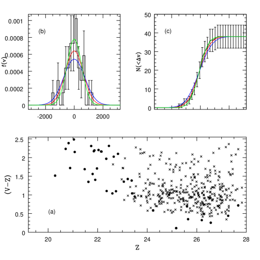
Figure 1: Upper left panel: binned velocity distribution of the spectroscopic members, compared to Gaussians with dispersion obtained through the biweight estimate (red) and considering the jackknife uncertainties (blue and green). All distributions are normalized to 1.0. Upper right panel: cumulative velocity distributions, colour code as in the left panel. Lower panel: observed colour magnitude diagram of GN 5 of all spectroscopic (black circles) and photometric (crosses) members of the cluster within 1 Mpc from the center.

Figure 2: Density isosurfaces for structures at $z\sim 0.45-0.48$ a), at $z\sim 0.64$ b), $z\sim 0.85$ c) and at $z\sim 0.97-1.01$ d) (average, average $+2\sigma$, average $+3\sigma$ to average $+10\sigma$) superimposed on the ACS z850 band image of the GOODS-North field. Yellow crosses indicate the density peak of each structure, the number is the ID of the structure in Table 1.

Figure 2 shows the density isosurfaces for the structures in GOODS-North superimposed on the ACS z850 band images of the field. Figure 3 shows the positions of the overdensities over the photometric redshift distribution of the entire GOODS-North sample. The overdensities are also traced by the distribution of the spectroscopically confirmed AGN in our catalogue, as shown in the lower panel of this Figure (note that AGN are not included in the sample used for the density estimation ). The analogous figures for GOODS-South were presented in Salimbeni et al. (2009).

2.3 X-ray emission from the clusters and groups

An inspection of the Chandra images at each cluster/group position shows that only two of the structures have significant extended X-ray emission due to the hot IGM. These are cluster GS 5 and cluster GN 8. The emission from Cluster GS 5 can be modeled with a Raymond Smith model with a best fit temperature 2.6 keV and metallicity 0.2 $Z_{\odot}$: the resulting X-ray luminosity is $9.56\times 10^{42}ergs^{-1}$ in the 0.1-2.4 keV rest-frame band (Castellano et al. in preparation). For GN 8 we can not estimate a temperature from the data: in this case the X-ray luminosities in the 0.1-2.4 keV rest-frame band is 4.1$\times 10^{42}ergs^{-1}$, assuming a Raymond Smith model with temperature 1 keV and metallicity 0.2 $Z_{\odot}$. All other structures, including the most massive ones, are undetected: as argued by Salimbeni et al. (2009), this lack of X-ray emission possibly indicates that optically selected structures are X-ray under-luminous, at least when compared to X-ray selected ones. This is for example the case of GS 4 (or CIG 0332-2747) at z=0.734, which was extensively discussed in Castellano et al. (2011), where we showed also a tentative $\sim 3\sigma$ detection of the X-ray emission, corresponding to a luminosity of $2\times 10^{42}ergs^{-1}$.
To further check the reality of our groups we performed a stack of the X-ray emission for all the new structures found in GOODS-North. We first measured the count rates in the soft band, within a square of side of $\sim$ $30\hbox{${}^{\prime\prime}$ }$ centred on the position of the peak of each structure, as given by our algorithm. This aperture was used to be consistent with Salimbeni et al. (2009) and corresponds approximately to a 1Mpc radius (of course depending slightly on redshift), which is similar to the $R_{200}$ reported in Table 1. We then masked all X-ray sources present within this area. We finally subtracted the soft-band background which was calculated from the total exposure map, by taking the total integration time at the position of each group and multiplying it by the average background count rate of 0.056 counts Ms^-1 pixel${-1}$ (Alexander et al. 2003). Alternatively for each group we calculated the average background count-rate in an annulus around the source where no other sources were present. The two values in general agreed to within 1%.
For the combination of the 7 groups/clusters in GOODS-North that are individually undetected (all but GN 8) we get an average of 310$\pm 60$ counts ($\sim 5.2\sigma$); if we only include the 5 groups that are used in this work, the result is 220$\pm 50$ ($\sim 4.4\sigma$). We convert the measured count rate to rest frame total $L_{x}$ in the 0.1–-2.4 keV band, assuming a metallicity $Z=0.3 Z_{\odot}$ and a temperature kT = 1 keV. This temperature is typical for low redshift groups with similar velocity dispersion (e.g. Osmond & Ponman 2004). We obtain a luminosity of the order 1-2 $10^{42}ergs^{-1}$. Compared to the typical luminosities of X-ray selected groups with similar velocity dispersion in the local Universe, the value we have found is on the low side, but still within the range of the X-ray luminosities of these structures (Osman & Ponman 2004).
We conclude that given the low mass of most of our structures and their high redshift, the lack of significant X-ray emission is still consistent in most cases with the $L_{x}-\sigma$ relation, especially if one considers the larger scatter that is found for optically selected structures (e.g. Rykoff et al. 2008). We caution that, although the results from the X-ray stacking are encouraging, it is impossible with the present data to test the virialization status of the individual groups.

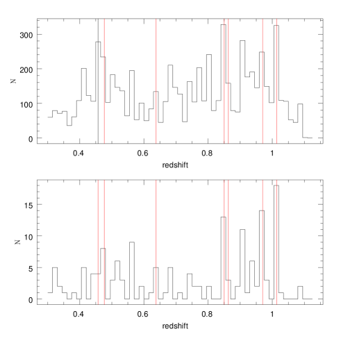
Figure 3: Upper panel: photometric redshift distribution of our sample (continuous line). The vertical red lines mark the redshifts of the detected structures. Lower panel: redshift distribution of spectroscopically selected AGN in the GOODS-North

ID	RA	Dec	redshift	$M_{R}$	Flux	Flux	Flux	${L_{H}}$	HR	Class	$log(f_{x}/f_{o})$
	2000	2000			tot	0.5-2 keV	2-8keV	$10^{42}ergs^{-1}$
GOODS-South
8355	53.1564	-27.8108	0.665	-22.28	-6.47e-17	1.71e-17	-9.85e-17	$<$0.19	$<$0.17	SB	-2.4
9633	53.1554	-27.7915	0.667	-22.68	-6.73e-17	2.10e-17	-9.59e-17	$<$0.18	$<$0.06	SB	-1.6
7031	53.0939	-27.8305	0.734	-19.5	4.00e-16	5.06e-17	3.29e-16	0.88	0.13$\pm$0.20	AGN2	0.0
8977	53.0734	-27.8033	0.734	-19.56	1.80e-16	-1.82e-17	2.39e-16	0.63	$>$0.42	AGN2	-0.66
9589	53.0618	-27.7940	0.735	-20.28	1.01e-16	2.87e-17	-1.54e-16	0.16	$<$0.14	AGN2	-0.85
9792	53.0751	-27.7885	0.734	-23.55	1.58e-16	8.33e-17	-1.20e-16	0.24	$<$-0.42	SB	-1.2
10995	53.0644	-27.7754	0.735	-20.71	-8.47e-17	2.73e-17	-1.31e-16	$<$0.35	$<$0.09	SB	-1.2
11184	53.1207	-27.7732	0.737	-20.24	6.66e-17	-2.33e-17	-1.40e-16	0.10	0.2$\pm 0.4$	AGN2	-0.22
11248	53.1197	-27.7723	0.738	-21.83	6.83e-16	2.66e-16	4.20e-16	1.12	-0.40$\pm 0.06$	AGN1	-0.22
11719	53.0769	-27.7655	0.738	-22.23	1.75e-16	-2.12e-17	2.14e-16	$>$ 0.57	$>$ 0.32	AGN2	-0.82
13053	53.0602	-27.7491	0.738	-20.00	4.50e-16	8.47e-17	3.70e-16	1.00	-0.02$\pm 0.2$	AGN2	0.73
13552	53.0941	-27.7405	0.738	-22.92	4.86e-16	3.55e-17	4.72e-16	1.26	0.44$\pm 0.3$	AGN2	-1.4
1837	53.0803	-27.9017	0.964	-23.71	4.2e-16	2.1e-16	-2.8e-16			cluster
11085	53.0658	-27.7749	1.021	-21.44	1.38e-16	4.72e-17	-1.61e-16	0.47	$<$-0.08	AGN2	-1.51
11285	53.0509	-27.7724	1.033	-22.38	2.60e-15	4.32e-16	2.22e-15	13.5	0.04$\pm$0.07	AGN2	0.23
3920	53.0715	-27.8724	1.097	-21.73	1.42e-14	4.98e-16	1.41e-14	99.7	0.69$\pm 0.06$	AGN2	1.03
GOODS-North
1795	188.9940	62.1842	0.638	-22.40	6.6e-16	1.20e-16	5.10e-16	0.97	-0.10$\pm 0.25$	SB	-1.1
2600	189.0136	62.1865	0.638	-22.74	4.1e-16	1.40e-16	-3.20e-16	0.45	$<$ -0.34	SB	-1.54
3349	189.0276	62.1643	0.637	-21.84	3.22e-15	-6.00e-17	3.30e-15	6.28	$>$ 0.74	AGN2	0.36
10013	189.1215	62.1796	1.013	-22.39	2.31e-15	1.70e-16	2.23e-15	12.9	0.34$\pm 0.15$	AGN2	0.57
11584	189.1403	62.1684	1.016	-23.09	8.60e-16	2.50e-16	6.00e-16	3.50	-0.32$\pm 0.09$	AGN1	-0.57
10066	189.1220	62.2706	0.848	-22.59	2.54e-15	1.20e-16	2.59e-15	9.79	0.51$\pm 0.18$	AGN2	-0.18
12018	189.1453	62.2746	0.848	-21.79	6.3e-16	4.00e-17	6.10e-16	2.31	0.41$\pm 0.38$	AGN2	-0.31
13907	189.1657	62.2634	0.848	-22.89	1.9e-16	9.00e-17	-1.70e-16	0.42	$<$-0.43	SB	-0.55
14867	189.1758	62.2627	0.857	-22.88	2.46e-15	6.9e-16	1.82e-15	7.07	-0.22$\pm 0.07$	AGN	0
16314	189.1926	62.2577	0.851	-22.12	5.6e-16	1.9e-16	3.40e-16	1.30	-0.42$\pm 0.10$	AGN	0.12
17850	189.2096	62.3347	1.011	-21.79	1.81e-15	6.7e-16	1.10e-15	6.36	-0.45$\pm 0.05$	AGN1	0.79
19243	189.2230	62.3386	1.023	-21.23	1.73e-15	3.0e-17	1.75e-15	10.40	0.7$\pm 0.40$	AGN2	0.45
29746	189.3410	62.1767	0.978	-21.17	2.11e-15	5.0e-17	2.11e-15	11.21	0.67$\pm 0.27$	AGN2	-0.15
36782	189.4461	62.2756	0.440	-22.08	4.2e-16	9.0e-17	5.80e-16	0.38	$<$0.05	SB	-1.2
38454	189.4950	62.2494	0.457	-20.18	6.4e-16	2.0e-16	4.70e-16	0.43	-0.33$\pm 0.20$	SB	-0.66

Table 2: X-ray sources associated to galaxies brighter than $M_{B}$=-20; the Xray properties of the sources have been derived from the Chandra Deep Field South 4-Megasecond Catalog (http://heasarc.gsfc.nasa.gov/W3Browse/chandra/chandfs4ms.html) and the Chandra Deep Field North 2-Megasecond Catalog (http://heasarc.gsfc.nasa.gov/W3Browse/all/chandfn2ms.html). The tipical on-axis 3$\sigma$ flux limits are $3.2\times 10^{-17}$, $9.1\times 10^{-18}$, and $5.5\times 10^{-17}ergcm^{-2}s^{-1}$ for the full, soft, and hard bands, respectively for the GOODS-South sources; $7.1\times 10^{-17}$, $2.5\times 10^{-17}$ and $1.4\times 10^{-16}ergscm^{-2}s^{-1}$ for the full, soft and hard bands for the GOODS-North sources. We refer to the linked table for individual flux uncertainties.

3 X-ray point sources identification and classification

Given the sensitivity of the 2 Msec observations with a typical total flux limit of 7 $\times 10^{-17}ergs^{-1}cm^{2}$, we are able to detect AGN with $L_{H}>10^{42}$ at all redshifts up to 1.1 (the most distant structure in the present study) also in the shallower GOODS-North field. We cross correlate the group/cluster member lists with the Chandra deep field north and south source catalogs derived respectively by Alexander et al. (2003) and Luo et al. (2008). The cross correlation was performed using a radius of 2 arcsec, which can be considered the nominal relative uncertainty of the astrometric solution. In all cases there is no ambiguity in the identification of the Chandra X-ray source with its optical counterpart.

Cluster	z	$\sigma$	$N_{spec}$	$N(M_{R}<-20)$	$N_{AGN}>10^{42}$	$\%$	$N_{AGN}>10^{43}$	$\%$
GS 1	0.666	390g	9	9	0	$<$13.2	0	$<$11.0
GS 4	0.735	600cl	65	59	3	5.1	0	$<$3.1
GS 5	0.966	420g	12	20	0	$<$9.2	0	$<$9.2
GS 6	1.038	630g	11	22	1	4.5	1	4.5
GS 8	1.098	510g	9	14	1	7.1	1	7.1
GN 1	0.638	590g	16	14	1	7.1	0	$<$13.1
GN 3	1.014	440cl	16	17	2	11.8	1	5.9
GN 5	0.851	600cl	37	45	4	8.9	0	$<$4.1
GN 6	1.014	370g	9	9	2	22.2	1	11.1
GN 7	0.973	370g	9	12	1	8.3	1	8.3
GN 8	0.457	570g	13	16	0	$<$11.5	0	$<$11.5
Total				237	15	6.3	5	2.1

Table 3: Cluster properties and AGN fraction; the velocity dispersion $\sigma$ is in km s^-1: “g” indicates that is was determined using gaussian statistics, while “cl” indicates that it was computed using the Gapper sigma statistics.

In Table 2 we present the group/cluster members with an absolute magnitude $M_{R}<-20$ which coincide with an X-ray source. AGN in galaxies fainter than this limit are not considered for consistency with previous works (e.g. Arnold et al. 2009). We find a total of 31 sources that are also members of our groups/clusters. In the Table we report their ID from the GOODS-MUSIC catalog for the southern field (Santini et al. 2009) and from Dahlen et al. (in preparation) for the northern field; the positions; the spectroscopic redshift; the total hard (2-8 keV) and soft band (0.5-2 keV) fluxes from the catalogs; the derived hardness ratio HR=(H-S)/(H+S), where H and S are the soft and hard band counts; the total inferred luminosity in the rest-frame hard band (2-10 KeV) obtained extrapolating the observed hard band flux and assuming a power law with photon index $\Gamma=1.8$. For those AGN which are undetected in the hard band, but are detected in the total band, this last value was used. For those few that are detected only in the soft band (and have upper limits both in the total and in the hard-band), we infer an upper limit for the total rest-frame hard band luminosity. Note that all these X-ray sources have a spectroscopic redshift.
The characterization of sources is not entirely trivial since we are probing deep enough X-ray luminosities that some of the detected X-ray emission might be due to star-burst rather than related to AGN activity (especially in the deeper GOODS-South field). We will employ a very simple classification according to the total luminosity and to the hardness ratio of the X-ray emission. X-ray sources are classified as type 2 AGN if they have a hardness ratio $HR\geq-0.2$, regardless of their total luminosity. They are classified as Type 1 AGN if they have $HS\leq-0.2$ but a total X-ray luminosity exceeding $10^{42}ergs^{-1}$. Sources with lower luminosity and soft emission, are classified as star-burst galaxies. In some case only a limit in available for the HR, so the classification becomes ambiguous: in this cases we further considered the X-ray-to-optical ratio ($log(f_{x}/f_{o})$), which is defined as the ratio between the total X-ray flux and the B band flux (as in Georgakakis et al. 2004). AGN broadly have $log(f_{x}/f_{o})$ in the range -1 to 1, so if $log(f_{x}/f_{o})<-1$, sources are considered star-burst. In Table 2 we report this ratio for all sources. We finally checked, whenever available in the literature, the optical spectra of the X-ray sources, or a classification based on these spectra (e.g. Szokoly et al. 2004, Trouille et al. 2008, Mignoli et al. 2004). Most of the sources are classified as emission line galaxies or high excitation emitters. None of the sources we could check were classified as broad line AGN.

In conclusion, of the total sample of X-ray sources, 9 are classified as star-burst galaxies, 15 are Type 2 AGN, 5 are Type 1 AGN, and one is associated to the diffuse emission from the hot cluster gas (although there could be a component associated to the BC galaxy). In some cases the classification maybe border line, however the AGN that we will use in the rest of the analysis (those with $L>10^{42}ergs^{-1}cm^{-2}$) all have a solid classification.

4 Results and discussion

4.1 AGN fractions in clusters and groups

We determine the fraction $f_{A}$ of AGN in clusters and groups, by dividing the number of AGN (regardless of type) by the total number of members down to an absolute magnitude limit $M_{R}=-20$. All AGN have a spectroscopic redshift, but cluster/group members include also some galaxies with only a photometric redshift. While it is possible that some of the galaxies included are interlopers, we also expect that galaxies belonging to the structure could be placed out of the structures due to a wrong photometric redshift. We will assume that these two effects more or less compensate each other; in any case since we include only structures with at least 65% of spectroscopic members, we estimate that this uncertainty is minimal.
Another way to estimate the global structure population is from the velocity dispersion, using the correlation between this quantity and the total number of galaxies within $R_{200}$ found by Koester et al. (2007) which is $ln\sigma=5.52+0.31lnN_{R200}$. We derive the $N_{200}$ using this relation and it is in general agreement with the total number of cluster/group members derived from our photometric plus spectroscopic redshifts.
In Table 3 we report the fraction of AGN with luminosity larger than $L_{H}=10^{42}ergs^{-1}$ and the fraction of AGN with luminosity higher than $L_{H}=10^{43}ergs^{-1}$, hosted by galaxies with rest-frame magnitude brighter than $M_{R}=-20$. When no AGN are identified the upper limits are evaluated using the low number statistics estimators by Gehrels (1986). Overall, we find an average fraction of $6.3\%$ for AGN with $L_{H}>10^{42}ergs^{-1}$ with a very large range (from less than $5\%$ to $22\%$). For the most luminous AGN with $L_{H}>10^{43}ergs^{-1}$, we find a global fraction of $2.1\%$. In Figure 4 we plot these individual fractions (for $L_{H}>10^{42}ergs^{-1}$ ) or upper limits for our groups and small clusters (as green symbols).

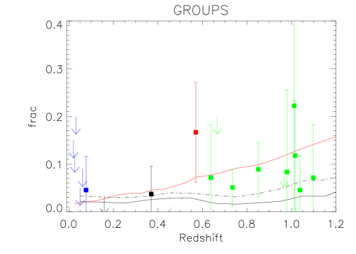
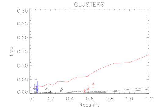
Figure 4: Left panel: the fraction of AGN with $L_{H}>10^{42}ergs^{-1}$ in groups and small clusters with velocity dispersion $350<\sigma<700\ kms^{-1}$. Green symbols are structures from the present work, blue symbols are from Arnold et al. (2009), black symbols from Martini et al. (2009), red symbol from Eastman et al. (2007). Right panel: the same for clusters with $\sigma>700\ kms^{-1}$. In both plots, to determine the upper limits and to estimate the uncertainties on the fractions we used the low number statistics estimators (at 1 $\sigma$) by Gehrels (1986). The red solid lines are the predictions from the Millenium simulation (Guo et al. 2011), the black solid and dash-dotted lines are the nominal and maximal predictions using the Menci et al. (2006) model, see text for more details.

4.2 The dependence of AGN fractions on redshift and velocity dispersion

Our results can be immediately compared to the analogous analysis of low redshift groups and clusters by Arnold et al. (2009). They selected structures with a range of velocity dispersions (and richness) similar to ours and extended to groups with $\sigma$s as low as 250 km/s and, on the other side, to few more massive clusters with $\sigma$ up to 900$kms^{-1}$. For a more accurate comparison we restrict their study to the same range of velocity dispersion probed by our sample, which is approximately between $350$ and 700$km/s$, thus including six of their structures. The result is a fraction of AGN with $L_{H}>10^{42}ergs^{-1}$ of $\sim 1\%$ at an average redshift z=0.045. No AGN brighter than $L_{H}=10^{43}ergs^{-1}$ are hosted by groups and small clusters in the local universe in the sample of Arnold et al. (2009), implying a limit of $<0.9\%$. In Figure 4 we report the values derived by Arnold et al. for these six groups (represented as blue symbols); we also include few more relevant results from the literature, in particular the small clusters presented in Martini et al. (2009) at slightly higher redshift (Abell 1240 at $z=0.159$ and MS1512 at $z=0.37$, black symbols) and one of the structures studied in Eastman et al (2007) (Abell 0848 at z=0.67, red symbol), with a velocity dispersion that is within our range. The trend for increasing AGN fraction with redshift is clear: most of the low redshift groups have no AGN (and are plotted as upper limits), while at $z>0.5$ many have $f_{A}\sim 5-10\%$ amongst bright galaxies. Note that in some cases, the luminosity of AGN in the above papers was reported in different rest-frame bands: we convert it to 2-10 KeV rest-frame, always assuming that the spectrum is represented by a power-law with photon index $\Gamma=1.8$ as above.
The same trend we observe in groups/small clusters has already been noted in more massive clusters: Eastman et al. (2007) compared the AGN content in clusters at z$\sim$0.6-0,7 to the analogous structures in the local Universe analysed by Martini et al. (2007) and found a factor of 10 increase. In Figure 4 (right panel) we also plot a collection of results from the literature on more massive structures (i.e. clusters with $\sigma>700kms^{-1}$): these include the three more massive clusters in Eastman et al. (2007) at z$\sim$0.6-0.7 (red symbols), the low redshift structures with $\sigma>700km/s$ from Arnold et al. (2009) (blue symbols) and the intermediate redshift clusters analysed by Martini et al. (2006) (black symbols). Although several results have been published on massive clusters at redshift above 0.7, we do not include them in this plot mainly because the available X-ray observations are not sensitive to AGN with luminosities of $L_{X}=10^{42}$ at these very high redshifts. We remind that for AGN with $L>L_{H}=10^{43}ergs^{-1}$ in clusters, Martini et al. (2009) found a considerable evolution from 0.2% at $z<0.3$ to 1.2 % at $z\sim 1$.
We conclude that groups behave like their more massive counterparts, in terms of AGN content and its evolution with time, and there is a net trend for an increasing AGN fraction hosted by galaxies brighter than a fixed limit ($M_{R}=-20$ in our case).

From a comparison between the two panels of Figure 4 we see that groups contain comparatively many more AGN that more massive clusters. To test if the fraction of AGN depends significantly on the velocity dispersion of the systems at a fixed redshift, we run a Spearman rank correlation: we first apply the test to our own sample and the result is a rank coefficient r=-0.58 with a probability of no correlation of P=0.06. So there are indications of some anti-correlation between the velocity dispersion of a structure and its AGN fraction, although with a large scatter. We then add the four structures studied by Eastman et al. (2007) at z$\sim$ 0.6 which include three higher velocity dispersion systems (see above). We repeated the Spearman rank correlation test with the total sample of 15 groups and clusters and found a higher coefficient (r=-0.64) with a much higher significance (P=0.010). We therefore conclude that, at a given redshift, the lower dispersion systems have comparatively more AGN at a fixed luminosity threshold, compared to the more massive structures.

4.3 The AGN spatial and velocity distribution within groups

The distribution of the AGN within the clusters and groups in terms of spatial position and relative velocity, can potentially offer clues on the triggering of the active phase, its lifetime, and the fueling mechanisms. If AGN are mainly fueled by galaxy-galaxy interactions, one expects that they should be more prevalent in the outskirts of clusters/groups. If gas-rich mergers are the primary mechanism for activating and fueling AGN, one expects higher AGN fractions in environments where galaxies have an abundant supply of gas: in this case galaxies in the centers of rich clusters should host less AGN since there is proportionally less cold gas (e.g. Giovanelli & Haynes 1985). However, a significant fraction of early type galaxies, which tend to lie in the centers of richest clusters, are known to harbour AGN and LINERs. A relation between AGN and early-type galaxies could dilute or even reverse the trends predicted by gas-rich mergers or galaxy harassment. A further effect that can trigger AGN is the interaction with the central brightest cluster galaxy, which is itself often a powerful AGN (e.g. Ruderman & Ebeling 2005). The relative importance of all these effects could also vary from very massive structures (where the velocity differences are more marked) to groups and smaller clusters.

Martini et al. (2002) were amongst the first to study the spatial distribution of X-ray selected AGN in clusters of galaxies at z $\sim$0.06-0.31 and found that the AGN with $L_{X}>10^{42}ergs^{-1}$ and $M_{R}<-20$ were located more centrally compared to inactive galaxies, although they had comparable velocity and substructure distributions to other cluster members. Ruderman & Ebeling (2005) studied the spatial distribution of X-ray point sources in 51 massive galaxy clusters at $0.3<z<0.7$, and concluded that they lie predominantly in the central 0.5 Mpc. Similarly Martel et al. (2007) showed that the surface density of the X-ray sources in five massive X-ray clusters at z$\sim 0.8-1.2$ is highest in the inner regions and relatively flat at larger radii, although AGN tend to avoid the very inner cores of clusters, i.e. regions of $\sim 200kpc$. The same was found by Galametz et al. (2009) for bright X-ray AGN for $0.5<z<1.5$ galaxy clusters and by Bignamini et al. (2008) for RCS clusters at z$\sim 0.6-1$ also showing a significant excess of medium luminosity X-ray AGN close to the centroid of the X–ray emission.

Figure 5: The solid line shows the radial distribution of all galaxies brighter than $M_{R}=-20$ in the 11 structures (normalized by the maximum radius of each structure); the dashed line is the same distribution for AGN

At variance with the above works, Gilmour et al. (2009) analysed a sample of 148 galaxy clusters at $0.1<z<0.9$ finding that the X-ray sources are quite evenly distributed over the central 1 Mpc, while Johnson et al. (2003) found that in the z$=$0.83 cluster $MS1054−0321$, the excess of X-ray AGN is at much larger radial distances, suggesting that they may be associated with infalling galaxies. Finally we mention the recent work of Fassbender et al. (2012) in high redshift massive clusters, indicated significant excess of low luminosity AGN in the inner (1Mpc) regions as well as an excess of brighter soft band sources at much larger distances suggesting perhaps the idea of two different AGN populations and triggering mechanisms of nuclear activity.

A big caveat to the above studies (with the exception of Martini et al. 2002, 2007) is the lack the spectroscopic redshift confirmation for most or all X-ray AGN. Moreover a lot of the analysis reported are limited to very luminous AGN: testing the distribution of more “normal” AGN can probe whether the AGN activity is more related to the host galaxy properties, or to the environment. We therefore analysed the spatial distribution of active and inactive galaxies in our structures; we used as cluster/group centers the position given by the search algorithm, unless a clearer center is given by the presence of extended X-ray emission (as in the case of GS 5) or by the position of a dominant brightest galaxy. We then determined the distance of the AGN and inactive galaxies from the center and normalized it by the extent of each system. The resulting distribution for normal and active galaxies is presented in Figure 5. We see no indication for a concentration of AGN towards the cluster/group center compared to the entire galaxy population. The distribution of AGN is actually flatter than that of the underling population, i.e. there are comparatively more AGN in the outer parts of the structures. To determine whether the AGN sample is consistent with being randomly drawn from the parent sample of galaxies or not, we run a non parametric K-S test. We find that the probability of this event is very low P=0.055, so most probably the AGN are distributed differently from the underling global population. Our conclusion is therefore that moderately luminous AGN tend to preferentially reside in the outskirts of structures compared to normal galaxies.
One possibility is that these AGN might have just entered in the cluster/group potential: in this case we also expect that they would be on more radial orbits compared to the rest of the population. Following, e.g., Martini et al. (2009) we determine the cumulative velocity distribution for all AGN, normalised by the cluster velocity dispersion in each case ($v-v_{c}/\sigma$). We find that the distribution agrees well with a Gaussian, thus there is no evidence that the AGN have a larger velocity dispersion than the rest of inactive galaxies.

In conclusion we find that our AGN are preferentially located in the outskirts of the structures but have the same velocity distribution as the rest of the galaxy population. This would support to the idea that mergers and tidal interactions are one of the main instigators of AGN activity; AGN are preferentially located in intermediate density regions (outskirts of groups and clusters) which are the most conducive to galaxy-galaxy interactions because of the elevated densities, compared to the field, but the relatively low velocities compared to cluster cores. However given the many discrepant results in the literature, this scenario has to be tested further with larger, high redshift group samples.

4.4 The color-magnitude relation of AGN in dense environment

It has been proposed that AGN may be responsible for the moderation of star-formation activity, either by sweeping up the gas from the galaxy thus stripping star-formation, or by inhibiting further gas from cooling and infalling (e.g., Maiolino et al. 2012, Croton et al. 2006). In this context one can predict the AGN hosts to be located in distinct regions of the color-magnitude diagram for galaxies. In particular the color distribution of AGN compared to those of the general (inactive) galaxy population can place constraints on the relative timing of the physical processes that take place in the galaxies: for example, if the nuclear activity timescale is longer than the timescales on which star formation activity is quenched, or if there are dynamical delays between star-burst and AGN activity in galaxy nuclei, AGN hosts will tend to be preferentially red compared to the general inactive galaxy population.

We therefore investigated the colors of our AGN host galaxies compared to the underling galaxy population: we remark that our AGN are all of modest luminosities hence we expect that their optical light is dominated by host galaxy contribution and not influenced in a significant way by the AGN, therefore the colors we determine correspond to the stellar population. We further checked this issue by exploiting the fitting made by Santini et al. (2012) for X-ray sources in Goods-North and South. Here the spectral energy distribution (SED) of galaxies hosting Xray sources was fitted with a double component, one for the AGN and one for the stars (see for example Figure 2 of that paper, for two cases, a type 1 and a type 2 AGN). As a result we get for the best-fit solution the relative contribution to the total luminosity of the two components at a rest-frame wavelength 6500 Å(R-band). We have verified that for our sources the contribution of the AGN component is not significant in all cases.

The color-magnitude diagram for the X-ray sources and of the general galaxy population is shown in Figure 6: the galaxies show the well-established bimodality of colors at this redshift, while it is clear that X-ray sources are not randomly distributed over the same region as the galaxies. All AGN hosts have colors redder than $U-B>0.5$ and tend to reside mostly in the green valley, on the red sequence or the top of the blue cloud.

This plot can be immediately compared to an analogous one by Nandra et al. (2007, Figure 1 of their paper) who analysed the Color-Magnitude Relation for X-Ray selected AGN in the AEGIS field at a similar redshift ($0.6<z<1.4$). If we neglect the brightest of their AGN, which are actually QSOs and have very blue colors, we see that in their case AGN tend to populate the entire color magnitude diagram; there are also AGN in the blue cloud, although they are a relative minority. The fraction of galaxies which are also X-ray sources in the red sequence, green valley and blue cloud are 3.4, 4.2 and 0.9% respectively. Silverman et al. (2008) also showed that the fraction of galaxies hosting AGN peaks in the ”green valley” ($0.5<U-V<1.0$) especially in the presence of large scale structures. They further showed that at $z>0.8$, a distinct, blue population of host AGN galaxies is prevalent, with colors similar to the star-forming galaxies. More recently, Rumbaugh et al. (2012) confirmed that in clusters and superclusters many AGN are located in the green valley, consistent with being a transition population.

From the comparison of the color-magnitude diagram of AGN in groups/clusters (our work Figure 6) with the CMD of AGN in the field (Nandra et al., Silverman et al.) we can see that in groups/cluster the AGN basically avoid the blue cloud, while in the field, AGN are also present in the blue cloud. If merger-induced AGN activity is associated with the process that quenches star formation in massive galaxies (e.g. di Matteo et al. 2005), causing the migration of blue cloud galaxies to the red sequence (Croton et al. 2006; Hopkins et al. 2006b), then the different color-distribution of AGN in the field and in groups indicates that these phenomena are more rapid in dense environments. Galaxies hosting AGN abandon the blue cloud more rapidly in clusters and groups, as inferred from our data, compared to what happens in the field.

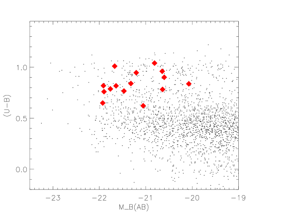
Figure 6: The color magnitude diagram for all galaxies in the clusters and groups (small black dots) with the positions of the AGN marked by the red diamonds.

Figure 7: The predicted color magnitude relation for all galaxies (top panel) and active galaxies (lower panel) with a hard X-ray luminosity larger than $10^{42}ergs^{-1}$ from the M04 model: contours are number densities. In the lower panel we overplot the AGN observed in our sample as red diamonds.

5 Comparison to model predictions

A comparison between the observed results and the predictions of semi-analytic models (SAM) that include AGN growth, can help us understand what are the main physical processes that drive the formation and the fueling of black holes. In the previous section we have derived that the frequency and colors of AGN depend quite strongly on the environmental density, with marked differences between field, groups and massive clusters. We will therefore compare our results to models that analyse the processes of AGN triggering and fuelling within a fully cosmological framework. Broadly, there are two main modes of AGN growth in these models: the so called “radio mode” and the “quasars mode”. The quasar mode applies to black hole growth during gas-rich mergers where the central black hole of the major progenitor grows both by absorbing the central black hole of the minor progenitor and by accreting the cold gas. In the radio mode, quiescent hot gas is accreted onto the central super-massive black hole; this accretion comes from the surrounding hot halo and is typically well below the Eddington rate. This model captures the mean behaviour of the black hole over timescales much longer than the duty cycle.

We will employ two different semi-analytic models, one that implements only the quasar mode and one that implements both. The model of Menci et al. (2004 M04 in the following) falls in the first category and is particularly tailored to follow the evolution of AGN. In this model the accretion of gas in the central black holes, is triggered by galaxy encounters, not necessarily leading to bound mergers, in common host structures such as clusters and especially groups; these events destabilize part of the galactic cold gas and hence feed the central BH, following the physical modeling developed by Cavaliere & Vittorini (2000). The amount of cold gas available, the interaction rates, and the properties of the host galaxies are derived as in Menci et al. (2002). As a result, at high redshift the proto-galaxies grow rapidly by hierarchical merging; meanwhile fresh gas is imported and the BHs are fueled at their full Eddington rates. At lower redshift, the dominant dynamical events are galaxy encounters in hierarchically growing groups; at this point refueling diminishes as the residual gas is exhausted, and the destabilizing encounters also decrease. This model successfully reproduces the observed properties of both galaxies and AGN across a wide redshift range (e.g. Fontana et al. 2006; Menci et al. 2008b; Calura & Menci 2009; Lamastra et al. 2010).
We further compare our results to the output of a SAM model implemented in the Milleniumn simulations (MS in the following) as in Guo et al. (2011). For black hole growth and AGN feedback they follow Croton et al. (2006), who implement both ‘quasar’ mode and ‘radio’ mode. In the “quasars mode” black hole accretion is allowed during both major and minor mergers, but the efficiency in the latter is lower because the mass accreted during a merger depends, among the other factors, on the ratio $m_{sat}/m_{central}$ (eq. 8 in Croton et al. 2006). In the “radio mode”, the growth of the super-massive black hole is the result of continuous hot gas accretion once a static hot halo has formed around the host galaxy of the black hole. This accretion is assumed to be continual and quiescent (see Croton et al. 2006 for more details).

From the two SAMs, we select all galaxies residing in massive halos (on the scale of groups and clusters), with rest-frame magnitudes brighter than $M_{R}=-20$ as in our observations. As for the real clusters and groups, we divide the simulated structures into those with a velocity dispersion between 400 and 700 $kms^{-1}$ (i.e., groups and small clusters) and those with sigma above 700 $kms^{-1}$ (massive clusters). From the simulations we actually know the total mass of the corresponding dark matter halos, which is related to the velocity dispersion via ${v_{c}}^{3}=(M/f(z))*(h/0.235)$, where $f(z)=H(z)/H_{0}$, with halo mass in unity of $10^{12}M\odot$ and v is in unity of 100 $kms^{-1}$. The SAMs provide the total bolometric luminosity of each AGN; to convert this into observed X-ray luminosity in the 2-10keV rest-frame band, we follow the relations found by Marconi et. al. (2004) applied to our luminosity limits ($L_{H}>10^{42}$ and $L_{H}>10^{43}$)
For all galaxies, the model computes the total stellar mass (M*): at each redshift we determine the mass corresponding to $M_{R}=-20$ from the relation between stellar mass and $M_{R}$ derived from the GOODS-South catalog (Grazian et al. 2006). We then use this mass to select mock galaxies brighter than $M_{R}=-20$. Since the mass-magnitude relation has a scatter we make two different predictions. In one case we use the best fit value of the mass-magnitude relation to determine $M_{R}$ and then select galaxies (filled curve in Figure 4, nominal prediction). In the second case we use the maximum stellar mass M* corresponding to $M_{R}=-20$ as a selection threshold. In this second way we select more massive galaxies and therefore the probability to find an AGN in the galaxies is higher. This is the upper envelope of our prediction (dashed curve in Figure 4, maximal prediction).The MS model gives directly the R magnitude of the mock galaxies so for this model we have only the nominal prediction. The resulting fractions of AGN with $L_{H}>10^{42}$ in groups and clusters hosted by galaxies brighter than $M_{R}=-20$ found in the two models are presented in Figure 4, along with the observed data.
The MS model tends to over-predict the fraction of AGN, especially for massive structures and at high redshift, while is it more in agreement with the data for groups. It also predicts a very marked increase of the AGN fraction with redshift, more pronounced than what is observed in the data. This steep increment is linked to the marked rise of major mergers (the only mergers considered for the quasar mode) towards high redshift. This model predicts a modest dependence of the AGN fraction on the velocity dispersion of the systems: for example at z$\sim 0.6$ simulated groups contain only $\sim$20% more AGN than the more massive structures, while the observed difference is much larger.
The M04 model predicts a milder increase of AGN fraction with redshift, both for massive and smaller systems: this is due to the fact that in this model minor mergers and close encounters are also very important and their frequency does not depend so strongly on redshift, since the small Dark Matter halos continue to merge frequently until low redshift. The M04 model tend to under-predict slightly the observed AGN fractions at all redshifts: the observed offset between the data and the predictions is approximately a factor of 3, both for clusters and for groups. This can be explained by the known problems of semi-analytic model that tend to overestimate the number of galaxies at the faint end of the luminosity function. In particular for the M04 model this discrepancy at the faint end was extensively discussed in Salimbeni et al. (2008) and is clearly observed at the magnitude limit that we are using in this study ($M_{R}=-20$).
The M04 model predicts a marked difference between groups and clusters: for example at z$\sim$0.6 groups/small systems contain a factor of 5 more AGN compared to massive clusters, in agreement with what is observed on the data. Indeed, in this model the fraction of gas accreted during mergers and fly-by is inversely proportional to the velocity dispersion of the structures, therefore for clusters it is lower than in groups. This effect is in addition to the increased merger rate between galaxies in groups, as compared to clusters, due to the lower encounter velocities in these small systems. In this sense, the agreement between the observational and predicted trends with velocity dispersion and with redshift validates the implemented mode of AGN growth in the M04 models.

We further check if the models can reproduce the colors of the AGN in dense environments. To this aim, we find that the MS model has problem in reproducing the colors of the general galaxy population in clusters and groups. Guo et al. (2011) already remarked clear differences between SDSS observations and model predictions in the slope of the red sequence and in the number of fainter red-sequence galaxies. The same was also noticed by de la Torre et al. (2011), who found that the De Lucia & Blazoit (2007) implementation on the Millenium Simulation does not reproduce quantitatively the observed intrinsic colour distributions of galaxies, with much fewer very blue galaxies and many more “green valley” galaxies in the model than in the observations, at redshifts $0.2<z<2.1$. In addition, the model predicts an excess of red galaxies at low redshift. We therefore decided to employ only the M04 model for this comparison: this model does a good job in reproducing the color bimodality of galaxies up to high redshift, as shown in the upper panel of Figure 7 where we plot the predicted color magnitude relation for all mock galaxies. The galaxies are located in a clear red-sequence and blue cloud and are well matched to the colors of the observed galaxies (Figure 6).

In the lower panel we plot the predicted colors of active galaxies which are selected as objects with a total rest-frame magnitude brighter than $M_{R}=-20$, hosting an AGN with luminosity exceeding $10^{42}ergs^{-1}$, and included in halos of mass comparable to our small clusters and groups. Here we also plot the colors of our observed AGN.

The U-B color range of the predicted AGN is well matched to the observations, most AGN having $0.5<U-B<1$, like the observed ones. The model predicts the presence of a small fraction of extremely red AGN, that reside on top of the red sequence, i.e., that are even redder than the typical red-sequence galaxies. We do not observe these extremely red AGN but this might be just due to lack of statistics. The model also predicts AGN in galaxies brighter than $M_{U}V=-22$ that we do not observe. Again this could be due to lack of statistics, since these extremely luminous galaxies are quite rare in our observed sample (see Figure 6). Alternatively it might be that mock galaxies hosting AGN of $L\sim 10^{42}ergs^{-1}$ become too bright. Indeed in the M04 model each encounter/merger that triggers AGN activity also triggers star-formation, thus enhancing the UV luminosity of the host galaxy; the relative proportion of gas that feeds AGN and star formation, which is now fixed to approximately 1 to 4 (see Menci et al. 2006) might need to be revised.

6 Summary and conclusions

We have explored the AGN content in small clusters and groups in the two GOODS fields, exploiting the ultra-deep 2 and 4 Msec Chandra data and the deep multiwavelength observations available. We have used our previously tested cluster-finding algorithm to identify structures, exploiting the available spectroscopic redshifts as well as accurate photometric redshifts. We identified 9 structures in GOODS-south (already presented in Salimbeni et al. 2009) and 8 new structures in the GOODS-north field. To have a reliable estimate of AGN fraction, we restrict our study to structures where at least 2/3 of the galaxies brighter than $M_{R}=-20$ have a spectroscopic redshift. We identified those clusters members that coincide with X-ray sources in the 4 and 2 Msec source catalogs (Luo et al. 2011 and Alexander et al. 2003 respectively), and with a simple classification based on total rest-frame hard luminosity and hardness ratio we determined if the X-ray emission originates from AGN activity or it is related to the galaxies’star-formation activity. We then computed the frequency of AGN in each group: we found that at $z\sim 0.6-1.0$ the average fraction of AGN with $LogL_{H}>42$ in galaxies with $M_{R}<-20$ is $6.3\pm 1.3\%$, i.e. much higher than the value found in lower redshift groups, which is just 1%. This fraction is also more than double the fraction found in more massive clusters at a similar redshift. We have then explored the AGN spatial distribution within the structures and found that they tend to populate the outer regions rather than the central cluster galaxies. The colors of AGN in structures are confined to the green valley and red-sequence, avoiding the blue-cloud, whereas in the field AGN are also present in the blue cloud (e.g. Nandra et al. 2007). If the AGN activity is associated with the process that quenches star formation in massive galaxies (e.g. di Matteo et al. 2005), causing the migration of blue cloud galaxies to the red sequence (Croton et al. 2006; Hopkins et al. 2006), we conclude that these phenomena are more rapid in dense environment compared to what happens in the field.

We finally compared our results to the predictions of two sets of semi analytic models: the M04 model (Menci et al. 2006) and one implemented on the Millenium Simulation by Guo et al. (2011). The MS model predicts a dependence of AGN content with redshift (both for clusters and groups) that is much steeper than what observed and a very modest difference between massive and less massive structures. The MS04 does a good job in predicting the redshift dependence of the AGN fractions, and the marked difference that is observed between groups and massive clusters. This agreement validates the implemented mode of AGN growth in the model and in particular stresses the importance of galaxy encounters, not necessarily leading to mergers, as an efficient AGN triggering mechanism.

The M04 model also reproduces accurately the range of observed AGN colors and their position in the color-magnitude diagram, although it tends to find AGN in galaxies that are on average slightly more luminous than the observed ones. It also predicts the presence of a small fraction of extremely red AGN, residing on top of the red sequence. We do not observe these extremely red AGN but this might be due to lack of statistics: we therefore plan to expand our analysis to other fields, with similar multiwavelength data and deep X-ray observations to study the AGN content. In particular we are currently working on the UDS field, thus more than doubling the area (and the statistics) presented of this paper. In this way we will be able to test, amongst other things, if the predicted extremely red AGN exist, and we will be able to place more stringent constrains on the relative timing of AGN activity and the quenching of star formation at high redshift.

References

- Alexander et al. (2003) Alexander, D. M., Bauer, F. E., Brandt, W. N., et al. 2003, AJ, 126, 539
- Andreon et al. (2009) Andreon, S., Maughan, B., Trinchieri, G., & Kurk, J. 2009, A&A, 507, 147
- Arnold et al. (2009) Arnold, T. J., Martini, P., Mulchaey, J. S., Berti, A., & Jeltema, T. E. 2009, ApJ, 707, 1691
- Balestra et al. (2010) Balestra, I., Mainieri, V., Popesso, P., et al. 2010, A&A, 512, A12
- Barger et al. (2008) Barger, A. J., Cowie, L. L., & Wang, W. 2008, ApJ, 689, 687
- Barnes & Hernquist (1996) Barnes, J. E. & Hernquist, L. 1996, ApJ, 471, 115
- Bauer et al. (2002) Bauer, F. E., Alexander, D. M., Brandt, W. N., et al. 2002, AJ, 123, 1163
- Beers et al. (1990) Beers, T. C., Flynn, K., & Gebhardt, K. 1990, AJ, 100, 32
- Bignamini et al. (2008) Bignamini, A., Tozzi, P., Borgani, S., Ettori, S., & Rosati, P. 2008, A&A, 489, 967
- Bird & Beers (1993) Bird, C. M., & Beers, T. C. 1993, AJ, 105, 1596
- Calura & Menci (2009) Calura, F., & Menci, N. 2009, MNRAS, 400, 1347
- Castellano et al. (2011) Castellano, M., Pentericci, L., Menci, N., et al. 2011, A&A, 530, A27
- Castellano et al. (2007) Castellano, M., Salimbeni, S., Trevese, D., et al. 2007, ApJ, 671, 1497
- Cavaliere & Vittorini (2002) Cavaliere, A., & Vittorini, V. 2002, ApJ, 570, 114
- Croton et al. (2006) Croton, D. J., Springel, V., White, S. D. M., et al. 2006, MNRAS, 365, 11
- Dawson et al. (2001) Dawson, S., Stern, D., Bunker, A. J., Spinrad, H., & Dey, A. 2001, AJ, 122, 598
- de la Torre et al. (2011) de la Torre, S., Meneux, B., De Lucia, G., et al. 2011, A&A, 525, A125
- De Lucia & Blaizot (2007) De Lucia, G., & Blaizot, J. 2007, MNRAS, 375, 2
- Di Matteo et al. (2005) Di Matteo, T., Springel, V., & Hernquist, L. 2005, Nature, 433, 604
- Dressler & Shectman (1988) Dressler, A., & Shectman, S. A. 1988, AJ, 95, 985
- Eastman et al. (2007) Eastman, J., Martini, P., Sivakoff, G., et al. 2007, ApJ, 664, L9
- Eisenhardt et al. (2008) Eisenhardt, P. R. M., Brodwin, M., Gonzalez, A. H., et al. 2008, ApJ, 684, 905
- Elbaz et al. (2007) Elbaz, D., Daddi, E., Le Borgne, D., et al. 2007, A&A, 468, 33
- Fassbender et al. (2012) Fassbender, R., Suhada, R., & Nastasi, A. 2012, arXiv:1203.5337
- Fontana et al. (2006) Fontana, A., Salimbeni, S., Grazian, A., et al. 2006, A&A, 459, 745
- Galametz et al. (2009) Galametz, A., Stern, D., Eisenhardt, P. R. M., et al. 2009, ApJ, 694, 1309
- Gehrels (1986) Gehrels, N. 1986, ApJ, 303, 336
- Georgakakis et al. (2004) Georgakakis, A., Georgantopoulos, I., Vallbé, M., et al. 2004, MNRAS, 349, 135
- Giavalisco et al. (2004) Giavalisco, M., Ferguson, H. C., Koekemoer, A. M., et al. 2004, ApJ, 600, L93
- Gilmour et al. (2009) Gilmour, R., Best, P., & Almaini, O. 2009, MNRAS, 392, 1509
- Gladders & Yee (2000) Gladders, M. D. & Yee, H. K. C. 2000, AJ, 120, 2148
- Grazian et al. (2006) Grazian, A., Fontana, A., de Santis, C., et al. 2006, A&A, 449, 951
- Guo et al. (2011) Guo, Q., White, S., Boylan-Kolchin, M., et al. 2011, MNRAS, 413, 101
- Hopkins et al. (2006) Hopkins, P. F., Hernquist, L., Cox, T. J., Robertson, B., & Springel, V. 2006, ApJS, 163, 50
- Koester et al. (2007) Koester, B. P., McKay, T. A., Annis, J., et al. 2007, ApJ, 660, 239
- Kurk et al. (2009) Kurk, J., Cimatti, A., Zamorani, G., et al. 2009, A&A, 504, 331
- Lamastra et al. (2010) Lamastra, A., Menci, N., Maiolino, R., Fiore, F., & Merloni, A. 2010, MNRAS, 405, 29
- Luo et al. (2008) Luo, B., Bauer, F. E., Brandt, W. N., et al. 2008, ApJS, 179, 19
- Mainieri et al. (2005) Mainieri, V., Rosati, P., Tozzi, P., et al. 2005, A&A, 437, 805
- Marconi et al. (2004) Marconi, A., Risaliti, G., Gilli, R., et al. 2004, MNRAS, 351, 169
- Martini et al. (2002) Martini, P., Kelson, D. D., Mulchaey, J. S., & Trager, S. C. 2002, ApJ, 576, L109
- Martini et al. (2006) Martini, P., Kelson, D. D., Kim, E., Mulchaey, J. S., & Athey, A. A. 2006, ApJ, 644, 116
- Martini et al. (2007) Martini, P., Mulchaey, J. S., & Kelson, D. D. 2007, ApJ, 664, 761
- Martini et al. (2009) Martini, P., Sivakoff, G. R., & Mulchaey, J. S. 2009, ApJ, 701, 66
- Menci et al. (2004) Menci, N., Fiore, F., Perola, G. C., & Cavaliere, A. 2004, ApJ, 606, 58
- Menci et al. (2002) Menci, N., Cavaliere, A., Fontana, A., Giallongo, E., & Poli, F. 2002, ApJ, 575, 18
- Menci et al. (2006) Menci, N., Fontana, A., Giallongo, E., Grazian, A., & Salimbeni, S. 2006, ApJ, 647, 753
- Mignoli et al. (2004) Mignoli, M., Pozzetti, L., Comastri, A., et al. 2004, A&A, 418, 827
- Nakamura (2000) Nakamura, T. K. 2000, ApJ, 531, 739
- Nandra et al. (2007) Nandra, K., Georgakakis, A., Willmer, C. N. A., et al. 2007, ApJ, 660, L11
- Osmond & Ponman (2004) Osmond, J. P. F., & Ponman, T. J. 2004, MNRAS, 350, 1511
- Popesso et al. (2009) Popesso, P., Dickinson, M., Nonino, M., et al. 2009, A&A, 494, 443
- Rykoff et al. (2008) Rykoff, E. S., McKay, T. A., Becker, M. R., et al. 2008, ApJ, 675, 1106
- Ruderman & Ebeling (2005) Ruderman, J. T., & Ebeling, H. 2005, ApJ, 623, L81
- Rumbaugh et al. (2012) Rumbaugh, N., Kocevski, D. D., Gal, R. R., et al. 2012, ApJ, 746, 155
- Salimbeni et al. (2009) Salimbeni, S., Castellano, M., Pentericci, L., et al. 2009, A&A, 501, 865
- Santini et al. (2009) Santini, P., Fontana, A., Grazian, A., et al. 2009, A&A, 504, 751
- Santini et al. (2012) Santini, P., Rosario, D. J., Shao, L., et al. 2012, A&A, 540, A109
- Shaw et al. (2006) Shaw, L. D., Weller, J., Ostriker, J. P., & Bode, P. 2006, ApJ, 646, 815
- Silverman et al. (2008) Silverman, J. D., Mainieri, V., Lehmer, B. D., et al. 2008, ApJ, 675, 1025
- Szokoly et al. (2004) Szokoly, G. P., Bergeron, J., Hasinger, G., et al. 2004, ApJS, 155, 271
- Trevese et al. (2007) Trevese, D., Castellano, M., Fontana, A., & Giallongo, E. 2007, A&A, 463, 853
- Trouille et al. (2008) Trouille, L., Barger, A. J., Cowie, L. L., Yang, Y., & Mushotzky, R. F. 2008, ApJS, 179, 1
- van Breukelen & Clewley (2009) van Breukelen, C. & Clewley, L. 2009, MNRAS, 395, 1845
- Vanderlinde et al. (2010) Vanderlinde, K., Crawford, T. M., de Haan, T., et al. 2010, ArXiv e-prints
- Vanzella et al. (2008) Vanzella, E., Cristiani, S., Dickinson, M., et al. 2008, A&A, 478, 83
- Vanzella et al. (2006) Vanzella, E., Cristiani, S., Dickinson, M., et al. 2006, A&A, 454, 423
- Xue et al. (2011) Xue, Y. Q., Luo, B., Brandt, W. N., et al. 2011, ApJS, 195, 10