Can car density in a two-lane section depend on the position of the latter in a single-lane road?

Abstract

We report here results on the study of the totally asymmetric simple exclusion processes (TASEP), defined on an open network, consisting of head and tail simple chain segments with a double-chain section inserted in-between. Results of numerical simulations for relatively short chains reveal an interesting new feature of the network. When the current through the system takes its maximum value, a simple translation of the double-chain section forward or backward along the network, leads to a sharp change in the shape of the density profiles in the parallel chains, thus affecting the total number of cars in that part of the network. In the symmetric case of equal injection and ejection rates $\alpha=\beta>1/2$ and equal lengths of the head and tail sections, the density profiles in the two parallel chains are almost linear, characteristic for the coexistence line (shock phase). Upon moving the section forward (backward), their shape changes to the one typical for the high (low) density phases of a simple chain. The total bulk density of cars in a section with a large number of parallel chains is evaluated too. The observed effect might have interesting implications for the traffic flow control as well as for biological transport processes in living cells. An explanation of this phenomenon is offered in terms of finite-size dependence of the effective injection and ejection rates at the ends of the double-chain section.

Keywords: TASEP; traffic flow models; non-equilibrium phase transitions; traffic on networks; biological transport processes

I Introduction

Traffic often takes place along linear tracks which are interconnected to form a network structure. However, in the presence of hard-core exclusion the collective behavior of such transportation networks is not yet well understood. Indeed, the role of junctions has been considered only recently on the example of simple networks involving no more than two junctions, see BPB ; PK05 or on self-similar tree-like topologies, see BM10 and references therein.

The idea of studying networks composed of chain segments, which exhibit the bulk behavior of an open TASEP under boundary conditions, given in terms of effective input and output rates, was first advanced in our work BPB . The network considered there consists of two vertices of degree 3: one of out-degree 2 and the other one of out-degree 1, connected by 2 chains of the same direction; the third edge of each of these vertices belongs to a directed chain coupled to a separate reservoir of particles, see Fig. 1. The appearance of correlation effects close to the ends of the chain segments, as well as of cross-correlations in the double-chain segment was demonstrated. The same approach was applied in Ref. PK05 to an open network consisting of one vertex of degree 3 and out-degree 1. The two incoming chains are coupled to one reservoir, and the outgoing one is coupled to another reservoir. Different versions of simple networks were studied in Refs. EPK08 and EPK09 . In the former reference two cases were investigated: (a) two vertices of degree 3 connected by three chains, one of which has the opposite direction to the remaining two (closed system); (b) two vertices of degree 3 connected by two chains with the same direction; the remaining incoming and outgoing chains are coupled to reservoirs with the same particle density (open counterpart). In Ref. EPK09 graphs containing vertices of degree 4 and out-degree 1, 2, and 3 were considered. The notion of particle-hole symmetry in the presence of a junction was carefully analyzed and an appropriate interpretation on the microscopic level was given. TASEP with parallel update on single multiple-input–single-output junctions has been investigated too WLJ08 . Clearly, the above works have treated TASEP on diverse, but simple fixed network topologies. The main concern was the construction of the phase diagram under different open boundary conditions.

Figure 1: (Color online) Schematic presentation of the considered system: TASEP, defined on an open network (solid black line), consisting of head $C_{1}$ and tail $C_{4}$ simple chain segments with a double-chain section ($C_{2}$ and $C_{3}$) inserted in-between. In the system, considered in BPB all the simple chain segments have equal lengths $L_{1}=L_{2}=L_{3}=L_{4}$ (more details are in the text). The light grey (green) dash-dotted line shows a version of the network, where the double-chain section has been translated forward by $\Delta L$ so that the head and tail simple chain segments have lengths: $L_{1}=L_{1}+\Delta L$ and $L_{4}=L_{4}-\Delta L$.

Complex networks have also been a focus of research in the last decade. Attention has been paid to the traffic fluctuation problem in networks: the dependence between the mean value of the of traffic passing through a node (or a link) in a time interval and its standard deviation has been studied. It has been recognized that in the evolving networks functional units may emerge, which may be represented by topologically distinct subgraphs, see KN09 and references therein. Different types of diffusive dynamics, like spreading of disease and traffic or navigated walks have been studied on different networks, see, e.g., T01 ; Getal02 ; NR04 . In particular, high-density traffic of information packets on sparse modular networks with scale-free subgraphs was studied, see TM09 . Most of the results of graph theory relevant to large complex networks were related to the simplest models of random graphs. A large amount of the research was devoted to scale-free networks, i.e., networks with power-law vertex degree distribution. Traffic rules on such graphs usually include particle creation at randomly selected nodes and mutually interacting random walks to different specified destinations, see Eetal05 . In NKP11 the authors studied the stationary transport properties of the TASEP with random-sequential update on complex networks, both deterministic and stochastic. The TASEP rules were generalized, by an obvious extension of the rules applied in BPB , to fixed connected networks of $N_{s}$ directed segments (each consisting of $L\gg 1$ sites) and $N_{v}$ nodes. The theoretical approach was based on a combination of models of complex networks with the well-known mean field (MF) results for the simple chains (’segments’) which are assumed to connect the vertices of the underlying directed graph. These chain segments, representing the edges of the network graph, have to be long enough to make reasonable the application of the MF results. At that, the correlations that may build up close to the nodes of the network have to be neglected.

Recently, applications to biological transport have motivated generalizations of the TASEP to cases when the entry rate is chosen to depend on the number of particles in the reservoir (TASEP with finite resources) CZ09 . Last year, the cases of multiple competing TASEPs with a shared reservoir of particles GCAR12 and with limited reservoirs of particles and fuel carriers BCR12 were studied too.

II Model and numerical simulation results

In the asymmetric simple exclusion process, hard-core particles move along one-dimensional lattice of sites, which can be occupied by one particle at most $\{\tau_{i}=0,1\},\,i=1,\dots,L$. The particle can move right (left) with probability $p$ $(1-p)$ to a nearest neighbor site, if the site is empty. In the extremely asymmetric case particles are allowed to move in one direction only — this is the totally asymmetric simple exclusion process (TASEP). Its steady states are exactly known for both open and periodic boundary conditions, for continuous-time and several kinds of discrete-time dynamics. Here, we focus our attention on the steady states of the open TASEP with continuous-time stochastic dynamics, modeled by the so called random-sequential update. For a review on the exact results for the stationary states of TASEP, under different kinds of stochastic dynamics, and its numerous applications, we refer the reader to RSSS ; ERS ; S01 .

Our goal here is to present some interesting new effects, observed in a TASEP, defined on a simple network, consisting of head and tail simple chain segments ($C_{1}$ and $C_{4}$) with a double-chain section ($C_{2}$ and $C_{3}$) inserted in-between. The model system is presented schematically in Fig. 1. The particle injection rate at the left end of the network is $\alpha$ and the particle ejection rate at the right end of the network is $\beta$. $P_{b}$ is the branching point — the last site $(i=L_{1})$ of the head chain segment $C_{1}$, where particles can take with equal probability $p_{j}$ the upper $C_{2}$ or the lower $C_{3}$ branch of the double-chain section. $P_{m}$ is the merging point (first site of the tail segment $i=L_{1}+L_{2}+1$), where the particles moving along the $C_{2}$ and $C_{3}$ chain segments merge. The particle current in the system is denoted by $J$ (it is in the same direction for both chains of the double-chain section).

Figure 2: (Color online) Density distribution $\rho(x)$ (from numerical simulations) along the different chain segments of the open network of the type, shown in Fig. 1, when $\alpha=0.75$, $\beta=0.75$. The solid (red) squares are the reference results for the network with the (MC,CL,MC) phase structure appearing when $L_{1}=L_{2}=L_{3}=L_{4}$. Simple translation of the double-chain section, while the lengths of the double chain segments $C_{2}$ and $C_{3}$ are kept fixed $L_{2}=L_{3}=50$, and also the length of the whole network is kept fixed at $L=150$ sites, causes a noticeable change of the density profiles of $C_{2}$ and $C_{3}$. Translation forward leads to a density distribution shape on $C_{2}$ and $C_{3}$ (shown with solid (green) down-triangles), characteristic of the LD phase, while translation backward to a density distribution (solid (blue) up-triangles), characteristic of the HD phase. For comparison the density distribution (in a MC phase) of a simple chain of length $150$ sites is also shown with empty grey circles of larger size.

Figure 3: (Color online) Nearest-neighbor correlations $F_{corr}$ in the network with a double-chain section as a function of the scaled distance $x$ for $\alpha=0.75$, $\beta=0.75$. The simulation results for $F_{corr}$ correspond to the density distributions, shown in Fig. 2, for the different positions of the double-chain section.

The phase structure of the network, studied in BPB when all the simple chain segments have equal length, $L_{1}=L_{2}=L_{3}=L_{4}$, is presented by the triplet $(X_{1},X_{2,3},X_{4})$, where $X_{n}\ (n=1,2,3,4)$ stands for one of the stationary phases of the simple chain segment $C_{n}$: LD — low density, HD — high density, MC — maximum current, and CL — coexistence line. Our analytical analysis of the allowed phase structures, based on the properties of single chains in the thermodynamic limit, and the neglect of the pair correlations between the nearest-neighbor occupation numbers at the junctions of the different chain segments, yielded 8 possibilities. Here we focus our investigation on 3 of the most interesting cases (MC,LD,MC), (MC,CL,MC), and (MC,HD,MC) which appear when the boundary rates satisfy the inequalities $\alpha>1/2,\ \beta>1/2$, corresponding to the maximum current phase of a single chain. We have shown that the phase state of the chains in the double-chain section depends on the effective injection rate $\alpha^{*}$ of particles at the first site of each of the chain segments $C_{2,3}$ and on the effective removal rate $\beta^{*}$ of particles from the last site of each of these chains. Our further studies of the system reveal a rather interesting property whenever the network with $L_{1}=L_{2}=L_{3}=L_{4}$ has the (MC,CL,MC) phase structure. One can change effectively the effective rates $\alpha^{*}$ and $\beta^{*}$ at the network junction points simply by changing the position of the double chain section along the network, while keeping fixed both: the total length $L$ of the network and the length $L_{2}=L_{3}=L_{d}$ of the double-chain section. This is clearly observable in Figs. 2–4. As one can see in Fig. 2, a simple translation forward of the double chain section leads to a density profile on $C_{2}$ and $C_{3}$ characteristic of the LD phase (shown with solid down-triangles), while translation backward induces a density profile characteristic of the HD phase (shown with solid up-triangles). As a reference, the results for the density profiles of the system with segments of equal length $L_{1}=L_{2,3}=L_{4}=50$ are shown with solid squares.

The characteristic change of the density profiles is accompanied also with the corresponding characteristic change in the nearest-neighbor correlation function $F_{corr}$, displayed in Fig. 3, for the same cases, as the ones shown in Fig. 2. For comparison the density distribution (in the MC phase) and nearest-neighbor correlations of a simple chain of length $L=150$ sites are also shown in both figures with empty grey circles of larger size. The Monte Carlo simulation results, presented here, are for a relatively small system of fixed total length $L=L_{1}+L_{2,3}+L_{4}=150$ sites and fixed size of the double-chain section, $L_{2}=L_{3}=50$. The ensemble averaging was performed over $200$ independent runs and $1.5\times 10^{6}$ Monte Carlo steps were omitted in order to ensure that the system has reached a stationary state.

Numerical study of a larger system with total length $L=300$ sites reveals even higher sensitivity of the density distribution $\rho(x)$ along the chains $C_{2}$ and $C_{3}$ of the double-chain section with respect to quite small changes of the loop position on the network, see Fig. 4. Already at $\Delta L=2$ one can observe a noticeable change in the density distribution.

Figure 4: (Color online) Density distribution $\rho(x)$ (simulation results) along the two equivalent chain segments of the double chain section for bigger size network (total length $L=300$ sites) at $\alpha=0.75$, $\beta=0.75$. The results show the increased sensitivity of the density distributions to even a very small position change $\Delta L$ of the double chain section. The solid (red) squares are the reference results for $L_{1}=L_{2}=L_{3}=L_{4}=100$ ($\Delta L$=0).

III Theoretical analysis

III.1 Mean field theory

The possible phase structure of the present network was analyzed in our paper BPB by using the exact results for simple bulk chains $C_{n}$, $n=1,2,3,4$, coupled to each other by means of effective injection and removal rates. To be specific, let $\tau_{i}^{(n)}$, $i=1,2,\dots,L_{n}$, denote the particle occupation number of site $i$ in chain $C_{n}$ which contains $L_{n}$ sites. Here we let the length of the double-chain defect $L_{2}=L_{3}\equiv L_{d}$ and the total length of the network $L_{1}+L_{d}+L_{4}\equiv L$ to be fixed. The mean field theory assumes that all $L_{n}$, $n=1,2,3,4$, are large enough, so that the average occupation number $\langle\tau_{i}^{(n)}\rangle(L;\alpha,\beta)$ of site $i\in C_{n}$ in the stationary state of the whole system, under injection rate $\alpha$ and removal rate $\beta$, can be identified with the average occupation number $\langle\tau_{i}^{(n)}\rangle(L_{n};\alpha^{*},\beta^{*})$ in the stationary state of a single chain of length $L_{n}$ under some effective injection ($\alpha_{n}^{*}$) and removal $(\beta_{n}^{*})$ rates. Note that at the open boundaries of the whole network the continuity of the current $J_{L}$ through the system implies

$$J_{L}=\alpha[1-\langle\tau_{1}^{(1)}\rangle(L_{1};\alpha,\beta)]=\beta\langle\tau_{L}^{(4)}\rangle(L_{4};\alpha,\beta).$$ (1)

Under the above assumptions, these equalities will be approximated by

$$J_{L}\simeq\alpha[1-\langle\tau_{1}^{(1)}\rangle(L_{1};\alpha,\beta_{1}^{*})]\simeq\beta\langle\tau_{L_{4}}^{(4)}\rangle(L_{4};\alpha_{4}^{*},\beta).$$ (2)

Similarly, by neglecting the nearest-neighbor correlations at the junctions of different chains, the current continuity equation yields the approximate equalities

$$J_{L}\simeq\langle\tau_{L_{1}}^{(1)}\rangle(L_{1};\alpha,\beta_{1}^{*})\left\{\frac{1}{2}\left[1-\langle\tau_{1}^{(2)}\rangle(L_{d};\alpha_{2}^{*},\beta_{2}^{*})\right]+\frac{1}{2}\left[1-\langle\tau_{1}^{(3)}\rangle(L_{d};\alpha_{3}^{*},\beta_{3}^{*})\right]\right\}$$

$$\simeq\left[\langle\tau_{L_{d}}^{(2)}\rangle(L_{d};\alpha_{2}^{*},\beta_{2}^{*})+\langle\tau_{L_{d}}^{(3)}\rangle(L_{d};\alpha_{3}^{*},\beta_{3}^{*})\right]\left[1-\langle\tau_{1}^{(4)}\rangle(L_{4};\alpha_{4}^{*},\beta)\right].$$ (3)

Hence, taking into account the equivalence of chains $C_{2}$ and $C_{3}$, we set $\alpha_{2}^{*}=\alpha_{3}^{*}=\alpha_{d}^{*}$, $\beta_{2}^{*}=\beta_{3}^{*}=\beta_{d}^{*}$, and define

$$\beta_{1}^{*}=1-\langle\tau_{1}^{(2,3)}\rangle(L_{d};\alpha_{d}^{*},\beta_{d}^{*}),\qquad\beta_{d}^{*}=1-\langle\tau_{1}^{(4)}\rangle(L_{4};\alpha_{4}^{*},\beta)$$

$$\alpha_{d}^{*}=\frac{1}{2}\langle\tau_{L_{1}}^{(1)}\rangle(L_{1};\alpha,\beta_{1}^{*}),\qquad\alpha_{4}^{*}=2\langle\tau_{L_{d}}^{(2,3)}\rangle(L_{d};\alpha_{d}^{*},\beta_{d}^{*}),$$ (4)

or, alternatively,

$$\beta_{1}^{*}=\frac{J_{L}}{\langle\tau_{L_{1}}^{(1)}\rangle(L_{1};\alpha,\beta_{1}^{*})},\qquad\beta_{d}^{*}=\frac{J_{L}}{2\langle\tau_{L_{d}}^{(2,3)}\rangle(L_{d};\alpha_{d}^{*},\beta_{d}^{*})}$$

$$\alpha_{d}^{*}=\frac{J_{L}}{2[1-\langle\tau_{1}^{(2,3)}\rangle(L_{d};\alpha_{d}^{*},\beta_{d}^{*})]},\qquad\alpha_{4}^{*}=\frac{J_{L}}{1-\langle\tau_{1}^{(4)}\rangle(L_{4};\alpha_{4}^{*},\beta)}.$$ (5)

Thus, definitions (4) express the effective injection (removal) rates of chains $C_{2,3}$, $C_{4}$ ($C_{1}$, $C_{2,3}$) in terms of the average occupation number of the last (first) site of the preceding (subsequent) chain, while definitions (5) express the corresponding effective injection (removal) rates in terms of the finite-size current and the average occupation number of the first (last) site of the same chain. The consistency of these definitions is a measure of the extent to which nearest-neighbor correlations at the junctions can be neglected.

The above equations essentially simplify when $L_{n}\gg 1$, $n=1,2,3,4$, by replacing the finite-size properties of the current and the density profiles with their thermodynamic counterparts. To this end we define

$$\rho_{in}^{(n)}(\alpha,\beta)=\lim_{L_{n}\rightarrow\infty}\langle\tau_{1}^{(n)}\rangle(L_{n};\alpha,\beta),\quad\rho_{out}^{(n)}(\alpha,\beta)=\lim_{L_{n}\rightarrow\infty}\langle\tau_{L_{n}}^{(n)}\rangle(L_{n};\alpha,\beta),$$

$$\rho_{bulk}^{(n)}(\alpha,\beta)=\lim_{L_{n}\rightarrow\infty}\frac{1}{L_{n}}\sum_{i=1}^{L_{n}}\langle\tau_{i}^{(n)}\rangle(L_{n};\alpha,\beta).$$ (6)

In this case the current is determined by the bulk densities (omitting the dependence on the injection and removal rates):

$$J=\lim_{L\rightarrow\infty}J_{L}=\rho_{bulk}^{(1,4)}(1-\rho_{bulk}^{(1,4)})=2\rho_{bulk}^{(2,3)}(1-\rho_{bulk}^{(2,3)}).$$ (7)

Hence, we find expressions for the possible bulk densities in terms of the current in the thermodynamic limit:

$$\rho_{bulk}^{(1)}=\rho_{\pm}(J),\qquad\rho_{bulk}^{(4)}=\rho_{\pm}(J),\qquad\rho_{bulk}^{(2,3)}=\rho_{\pm}(J/2),$$ (8)

where

$$\rho_{\pm}(J)=\frac{1}{2}\left(1\pm\sqrt{1-4J}\right).$$ (9)

In the most interesting case $\alpha>1/2$ and $\beta>1/2$, both chains $C_{1}$ and $C_{4}$ are in the maximum current (MC) phase BPB , when the exact results in the limit $L\rightarrow\infty$ yield

$$J=1/4,\quad\rho_{bulk}^{(1)}(\mathrm{MC})=\rho_{bulk}^{(4)}(\mathrm{MC})=1/2,$$

$$\rho_{in}^{(1)}(\alpha,\beta_{1}^{*})=1-\frac{1}{4\alpha},\quad\rho_{out}^{(1)}(\alpha,\beta_{1}^{*})=\frac{1}{4\beta_{1}^{*}},$$

$$\rho_{in}^{(4)}(\alpha_{4}^{*},\beta)=1-\frac{1}{4\alpha_{4}^{*}},\quad\rho_{out}^{(4)}(\alpha_{4}^{*},\beta)=\frac{1}{4\beta}.$$ (10)

In this case from Eq. (8) it follows that either $\rho_{bulk}^{(2,3)}=\rho_{-}(1/8)\simeq 0.146$ and the defect chains $C_{2,3}$ are in the low density (LD) phase, or $\rho_{bulk}^{(2,3)}=\rho_{+}(1/8)\simeq 0.854$ and the defect chains $C_{2,3}$ are in the high density (HD) phase.

Consider first the LD case, when

$$\rho_{in}^{(2,3)}(\alpha_{d}^{*},\beta_{d}^{*})=\rho_{bulk}^{(2,3)}(\alpha_{d}^{*},\beta_{d}^{*})=\alpha_{d}^{*},\quad\rho_{out}^{(2,3)}(\alpha_{d}^{*},\beta_{d}^{*})=\alpha_{d}^{*}(1-\alpha_{d}^{*})\beta_{d}^{*}.$$ (11)

Then, in the large $L$ limit Eqs. (4) and (5) yield

$$\alpha_{d}^{*}=\rho_{bulk}^{(2,3)}(\alpha_{d}^{*},\beta_{d}^{*})=\rho_{-}(1/8),\quad\beta_{1}^{*}=\frac{1}{8\alpha_{d}^{*}}=\rho_{+}(1/8),\quad\beta_{d}^{*}=\frac{1}{4\alpha_{4}^{*}}=\frac{1}{8\rho_{out}^{(2,3)}(\alpha_{d}^{*},\beta_{d}^{*})}.$$ (12)

Consider next the HD case, when

$$\rho_{in}^{(2,3)}(\alpha_{d}^{*},\beta_{d}^{*})=1-\beta_{d}^{*}(1-\beta_{d}^{*})/\alpha_{d}^{*},\quad\rho_{out}^{(2,3)}(\alpha_{d}^{*},\beta_{d}^{*})=\rho_{bulk}^{(2,3)}(\alpha_{d}^{*},\beta_{d}^{*})=1-\beta_{d}^{*}.$$ (13)

Then, the large $L$ limit of Eqs. (4) and (5) yields

$$\alpha_{d}^{*}=\frac{1}{2}\rho_{out}^{(1)}(\alpha,\beta_{1}^{*})=\frac{1}{8\beta_{1}^{*}},\quad\alpha_{4}^{*}=\frac{1}{4\beta_{d}^{*}}=2\rho_{+}(1/8),\quad\beta_{d}^{*}=1-\rho_{bulk}^{(2,3)}(\alpha_{d}^{*},\beta_{d}^{*})=\rho_{-}(1/8).$$ (14)

We see that in both cases there remain undetermined effective rates: in the low density case these are $\beta_{d}^{*}$ and the related $\alpha_{4}^{*}$, see Eq. (12), and in the high density case $\alpha_{d}^{*}$ and the related $\beta_{1}^{*}$, see Eq. (14). We explain this feature by the fact that the relation between the magnitudes of $\alpha_{d}^{*}$ and $\beta_{d}^{*}$ depends on the phase of the chains $C_{2,3}$ when chains $C_{1}$ and $C_{4}$ are in the maximum current phase. Then the current through the whole system attains its maximum value $J=1/4$ and the bulk densities in $C_{1}$ and $C_{4}$ take the only possible value $\rho_{bulk}^{(1)}=\rho_{bulk}^{(4)}=1/2$. However, the value of the current through each of the chains $C_{2,3}$, $J^{(}2,3)=J/2=1/8$ allows them to be either in the low density phase, when $\beta_{d}^{*}>\alpha_{d}^{*}=\rho_{-}(1/8)$, or in the high density phase, when $\alpha_{d}^{*}>\beta_{d}^{*}=\rho_{-}(1/8)$, or on the coexistence line, when $\alpha_{d}^{*}=\beta_{d}^{*}=\rho_{-}(1/8)$. This means that there is a degree of freedom due to the fact that the average density of particles in the chains $C_{2,3}$ is not fixed. In the next section we show how one can deduce the missing injection/ejection rate from the fit of the density profile with the exponential distribution predicted by the domain wall theory.

Our former computer simulations BPB have shown that in the symmetric case of $L_{1}=L_{4}=200$ and $\alpha=\beta>1/2$ the double-chain segment is found to be on the coexistence line $\alpha_{d}^{*}=\beta_{d}^{*}<1/2$ (known also as a shock phase) when a completely delocalized domain wall exists. In this case the local density profile is linear and changes in the interval from $\rho_{bulk}(\mathrm{LD})$ to $\rho_{bulk}(\mathrm{HD})$, so that $\rho_{d}(\alpha_{d}^{*},\alpha_{d}^{*})=1/2$. Evidently, for a finite-size system the effective rates depend on the lengths of all the chains, $L_{1}$, $L_{d}$ and $L_{4}$. Simple arguments lead to the conclusion that as $L_{1}\rightarrow 1$, the effective injection rate $\alpha_{d}^{*}$ monotonically increases, so that $\alpha_{d}^{*}\rightarrow\alpha/2>1/4$, while $\beta_{d}^{*}=\rho_{-}(1/8)<1/4$ does not change significantly if $L_{d}\gg 1$, the defect chains $C_{2,3}$ go into the high density phase. On the other hand, when $L_{4}\rightarrow 1$, $\beta_{d}^{*}$ monotonically increases, so that $\beta_{d}^{*}\rightarrow\beta>1/2$, while $\alpha_{d}^{*}=\rho_{-}(1/8)<1/4$ does not change significantly, the defect chains $C_{2,3}$ go into the low density phase. That is actually observed in our present computer simulations, the results of which are illustrated in Figs. 2. The noticeable deviations of the density profiles from the standard infinite chain counterparts are due to finite-size effects, as well as to the correlations that appear near the points of inhomogeneity of the network, see Fig. 3. The sensitivity of the effect increases with the length of the chains, see Fig. 4, since then the smeared phase transition in $C_{2,3}$ becomes sharper.

Some numerical data for a network with fixed $L=150$, $L_{d}=50$ and changing $L_{1}=100-L_{4}$, are given in Table 1. The values of $\alpha_{d}^{*}$ and $\beta_{d}^{*}$ are calculated from the finite-size numerical data for the local densities $\langle\tau_{L_{1}}^{(1)}\rangle$, $\langle\tau_{1}^{(4)}\rangle$, $\langle\tau_{1}^{(2,3)}\rangle$ and $\langle\tau_{L_{d}}^{(2,3)}\rangle$, by using equations (4) and (5) with $J_{L}=J(\mathrm{MC})=1/4$.

$\;L_{1}\;$	$\langle\tau_{L_{1}}^{(1)}\rangle$	$\langle\tau_{1}^{(4)}\rangle$	$\langle\tau_{1}^{(2,3)}\rangle$	$\langle\tau_{L_{d}}^{(2,3)}\rangle$	$\alpha_{d}^{*}$	$\alpha_{d}^{*}$	$\beta_{d}^{*}$	$\beta_{d}^{*}$
					from Eq. (4)	from Eq. (5)	from Eq. (4)	from Eq. (5)
25	0.472	0.856	0.436	0.856	0.236	0.222	0.144	0.146
50	0.299	0.824	0.175	0.791	0.150	0.152	0.176	0.158
75	0.281	0.590	0.144	0.429	0.140	0.146	0.410	0.291

Table 1.

As is seen, the relative values of the effective rates change with the defect position, according to our expectations, and properly describe the phase changes, observed in the density profiles. The largest numerical discrepancies are observed between the values of $\beta_{d}^{*}$ obtained from Eqs. (4) and (5) in the cases of networks with $L_{1}=50$ and $L_{1}=75$. Probably, they can be explained by taking into account the high nearest-neighbor correlations between the defect section and the tail chain.

III.2 Domain wall theory

According to the Domain Wall (DW) theory, the configurations of TASEP on a simple chain with open boundaries can be approximated by two regions, of low and high density, separated by a domain law of zero width KSKS , see also SA . Thus, all the configurations of a chain of $L$ sites can be labeled by a single integer $k=0,1,\dots,L$, such that sites $0\leq i\leq k$ belong to the low density phase with uniform density $\rho_{-}$, and sites $k+1\leq i\leq L$ belong to the high density phase with uniform density $\rho_{+}$. The extremal values of $k=0$ and $k=L$ are understood to label configurations corresponding to the pure high and low density phases.

We recall that the probability $P(k,t)$ for finding at time $t$ the domain wall at position $k$ satisfies a master equation with reflecting boundary conditions at $k=0$ and $k=L$. The corresponding stationary solution $P_{*}(k)$ has the simple exponential form

$$P_{*}(k)=r^{-k}/{\mathcal{N}},$$ (15)

where

$$r=\frac{\alpha(1-\alpha)}{\beta(1-\beta)}=\left\{\begin{array}[]{cc}\exp(-1/\xi),&\alpha<\beta\leq 1/2\\ \exp(1/\xi),&\beta<\alpha\leq 1/2\end{array}\right.,$$

where $\xi>0$ is the domain wall localization length; the normalization factor ${\mathcal{N}}$ is

$${\mathcal{N}}:=\sum_{k=0}^{L}r^{-k}=\frac{1-r^{-(L+1)}}{1-r^{-1}}.$$ (16)

Thus, the local density of particles $\rho(i):=\langle n_{i}\rangle$ is given by

$$\rho(i)=\rho_{+}{\mathcal{N}}^{-1}\sum_{k=0}^{i-1}r^{-k}+\rho_{-}{\mathcal{N}}^{-1}\sum_{k=i}^{L}r^{-k}=\rho_{-}+(\rho_{+}-\rho_{-})\frac{1-r^{-i}}{1-r^{-L-1}}.$$ (17)

This expression describes different shapes depending on the value of $r$.

(a) On the coexistence line (CL) $r=1$ and Eq. (17) yields the linear profile

$$\rho_{CL}(i)=\rho_{-}+(\rho_{+}-\rho_{-})\frac{i}{L+1},\qquad 1\leq i\leq L.$$ (18)

(b) In the low density (LD) phase $r<1$ and up to exponentially small corrections one obtains

$$\rho_{LD}(i)=\rho_{-}+(\rho_{+}-\rho_{-})r^{L-i+1},\qquad r<1,\qquad 1\leq i\leq L.$$ (19)

(c) In the high density phase $r>1$ and up to exponentially small corrections one obtains

$$\rho_{HD}(i)=\rho_{+}-(\rho_{+}-\rho_{-})r^{-i},\qquad r>1,\qquad 1\leq i\leq L.$$ (20)

We shall concentrate on the last two cases which will be considered on the macroscopic scale $i/L=x$. To this end it is convenient to introduce the parameter $t=\xi/L$ and rewrite expression (19) as

$$\tilde{\rho}_{LD}(x)=\rho_{-}+A\exp{[(x-1-1/L)/t]},\qquad L^{-1}\leq x\leq 1,$$ (21)

where, $\tilde{\rho}_{LD}(x)=\rho_{LD}(xL)$ and $A=\rho_{+}-\rho_{-}$. Similarly, expression (20) takes the form

$$\tilde{\rho}_{HD}(x)=\rho_{+}-A\exp{(-x/t)},\qquad L^{-1}\leq x\leq 1,$$ (22)

where, $\tilde{\rho}_{HD}(x)=\rho_{HD}(xL)$ and $A=\rho_{+}-\rho_{-}$.

The results from the interpretation of our numerical results on the local density profiles within the DW theory are explained in the following two subsections.

III.2.1 Interpretation of the density profile fit in the LD phase

The fit to the simulated local density profile by function (21) is shown in Fig. 5. Its very high quality yields reliable estimates of $\rho_{-}=\alpha_{d}^{*}\simeq 0.148$, $A=0.421\pm 0.002$ and $t=0.0488\pm 0.0003$, hence, $r=\exp(-1/\xi)\simeq 0.664$.

The value of $\alpha_{d}^{*}=0.148$ is in fairly good agreement with the average current $J^{(2,3)}=J^{max}/2$ through each of the chains $C_{2,3}$: $\alpha_{d}^{*}(1-\alpha_{d}^{*})\simeq 0.126$; the difference between 0.126 and the expected value $J^{max}/2=1/8$ through each of the chains of the double-chain section can be attributed to finite-size effects in a network of total length $L=150$.

Figure 5: (Color online) The simulation results for the particle density profile $\rho(x)$, $x=(i-L_{1})/L_{2}$, $i=L_{1}+1,L_{1}+2,\dots,L_{1}+L_{2}$, in the LD phase of a chain $C_{2,3}$ in the network, are shown by centered grey circles, the fit with the function (21) is shown by solid (red) line. The quality of the fit is characterized by the statistical criteria $\chi^{2}/DoF=1.0004\times 10^{-6}$ and $R^{2}=0.99963$.

The most important observation is that, by using the prediction of the DW theory,

$$\beta_{d}^{*}(1-\beta_{d}^{*})=\alpha_{d}^{*}(1-\alpha_{d}^{*})/r=J^{(2,3)}/r,$$ (23)

we can evaluate the effective ejection rate $\beta_{d}^{*}$ by solving the above equation at $r=0.664$, with the result

$$\beta_{d}^{*}=(1/2)[1-\sqrt{1-4J^{(2,3)}/r}]\simeq 0.255.$$ (24)

Note that this value satisfies the conditions for the existence of a LD phase, but differs significantly from the mean field estimates given in Table 1. To check the validity of the DW theory, we have performed computer simulations of TASEP on a single chain with injection and ejection rates $\alpha=0.148$ and $\beta=0.255$, respectively. The corresponding density profiles are compared in Fig. 6.

Figure 6: (Color online) Comparison of the simulation results for the particle density profile $\rho(i)$, $i=1,2,\dots,50$, in the LD phase of a chain $C_{2,3}$ in the network (shown by solid (red) circles) and an open simple chain (shown by solid (blue) squares) under the estimated rates $\alpha=0.148$ and $\beta=0.255$.

One sees a qualitatively very close behavior of the density profiles, although in the region of upward bending, close to the right-hand end of the chains, the local density at the single chain sites is considerably higher than the one at the corresponding sites of the $C_{2,3}$ branches. At the right end this difference reaches its maximum: $\rho^{2,3}(L_{2})\simeq 0.429$, while for the simple chain $\rho^{SC}(L_{2})\simeq 0.495$. The latter value is not influenced significantly by finite-size effects, because it coincides, within numerical accuracy, with the value of the density in the thermodynamic limit for a simple chain with the same boundary rates:

$$\lim_{L\rightarrow\infty}\rho_{LD}(L)=\alpha_{d}^{*}(1-\alpha)_{d}^{*}/\beta_{d}^{*}\simeq 0.494.$$ (25)

We explain the above discrepancy by the presence of nearest neighbor correlations between the last site of the chains $C_{2,3}$ and the first site of the tail chain $C_{4}$:

$$F^{(d,4)}_{nn}=\langle\tau_{L_{d}}^{(2,3)}\tau_{1}^{(4)}\rangle-\langle\tau_{L_{d}}^{(2,3)}\rangle\langle\tau_{1}^{(4)}\rangle.$$ (26)

From the exact expression for the current $J^{(2,3)}$ through each of the chains $C_{2,3}$ it follows that

$$\rho_{L_{d}}^{(2,3)}=\frac{J^{(2,3)}+F^{(d,4)}_{nn}}{1-\rho_{1}^{(4)}}.$$ (27)

Hence, by inserting the numerically evaluated $F^{(d,4)}_{nn}\simeq 0.048$ and $\rho_{1}^{(4)}\simeq 0.590$, we obtain $\rho_{L_{d}}^{(2,3)}\simeq 0.424$ which is fairly close to the simulations result $\rho^{2,3}(L_{d})\simeq 0.429$.

Finally we note that although the DW theory gives an excellent description of the density profile of chains in the LD phase, the maximum reached at the right-hand end of a long simple chain is lower than the bulk density $\rho_{+}=1-\alpha_{d}^{*}$ of the high-density phase that supports the same current for all $\alpha_{d}^{*}<\beta_{d}^{*}$:

$$\lim_{L\rightarrow\infty}\rho_{LD}(L)=\alpha_{d}^{*}(1-\alpha_{d}^{*})/\beta_{d}^{*}<(1-\alpha_{d}^{*})=\rho_{+}.$$ (28)

Indeed, the interpretation $A=\rho_{+}-\rho_{-}$, given by the DW theory, yields a value for the bulk density of the HD phase, $\rho_{+}=A+\rho_{-}\simeq 0.569$, which cannot support the current $J^{(2,3)}=J^{max}/2$.

III.2.2 Interpretation of the fit in the HD phase

The fit to the simulated local density profile by function (22) is shown in Fig. 7. Its excellent quality yields reliable estimates of $\rho_{+}=1-\beta_{d}^{*}\simeq 0.853>1/2$, $A=0.594\pm 0.002$ and $t=0.0570\pm 0.0002$, hence, $r=\exp(1/Lt)\simeq 1.42$.

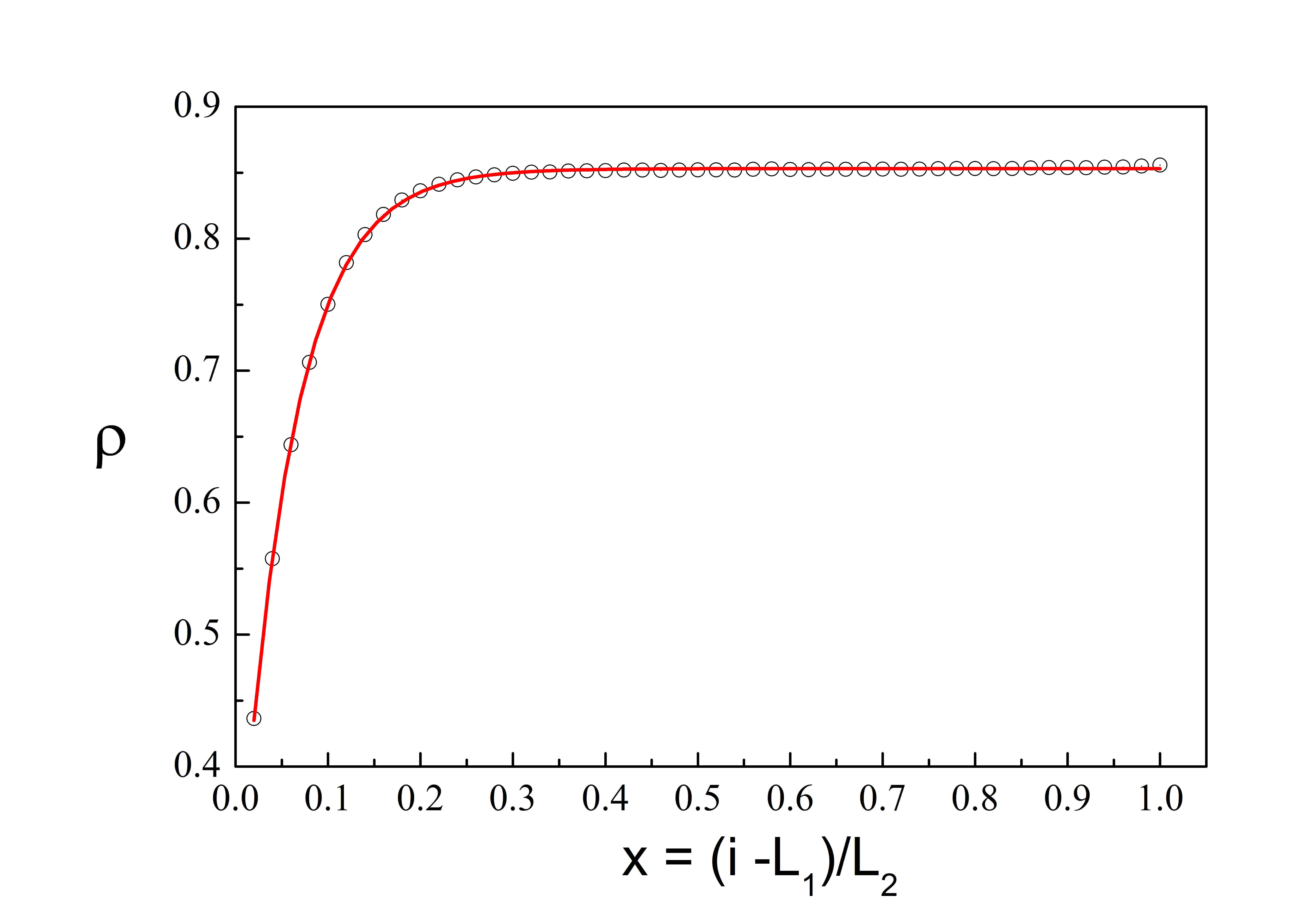
Figure 7: (Color online) The simulation results for the particle density profile $\rho(x)$, $x=(i-L_{1})/L_{2}$, $i=L_{1}+1,L_{1}+2,\dots,L_{1}+L_{2}$, in the HD phase of a chain $C_{2,3}$ in the network, are shown by centered grey circles, the fit with the function (22) is shown by solid (red) solid line. The quality of the fit is characterized by the statistical criteria $\chi^{2}/DoF=9.134\times 10^{-7}$ and $R^{2}=0.99986$.

From the relation for the bulk density in the HD phase, $\rho_{+}=1-\beta_{d}^{*}$, we deduce the value $\beta_{d}^{*}\simeq 0.147$ for the effective ejection rate. This gives a very good estimate of the current $J^{(2,3)}=\beta_{d}^{*}(1-\beta_{d}^{*})\simeq 0.1254$ through each of the chains $C_{2,3}$.

Next, following the DW theory, we solve the equation

$$\alpha_{d}^{*}(1-\alpha_{d}^{*})=r\beta_{d}^{*}(1-\beta_{d}^{*})=rJ^{(2,3)}$$ (29)

at $r=1.42$, to obtain

$$\alpha_{d}^{*}=(1/2)[1-\sqrt{1-4rJ^{(2,3)}}]\simeq 0.232.$$ (30)

This value agrees fairly well with the mean field estimates given in Table 1.

To check the consistency of the fit, from Eq. (20) we obtain

$$\rho_{-}\simeq\rho_{HD}(1)=\rho_{+}-A/r\simeq 0.435,$$ (31)

which almost coincides with the numerical value of $0.436$ for the density at the first site of the chains $C_{2,3}$. On the other hand, the analytical expression for the density profile in the thermodynamic limit leads to the estimate

$$\lim_{L\rightarrow\infty}\rho_{HD}(1)=1-\beta_{d}^{*}(1-\beta_{d}^{*})/\alpha_{d}^{*}\simeq 0.459,$$ (32)

which coincides, within numerical accuracy, with the numerical value $\rho^{SC}_{HD}(1)\simeq 0.460$ obtained for a simple chain under the same boundary rates, see Fig. 8, and which is about 5 percent higher than the numerically obtained value $\rho_{HD}(1)=0.436$. This small discrepancy is due to the small nearest-neighbor correlations between the last site of the head chain and the first site of chains $C_{2,3}$:

$$F^{(1,d)}_{nn}=\langle\tau_{L_{d}}^{(1)}\tau_{1}^{(2,3)}\rangle-\langle\tau_{L_{d}}^{(1)}\rangle\langle\tau_{1}^{(2,3)}\rangle=\simeq 0.011.$$ (33)

To check the validity of the DW predictions, we have simulated the density profiles in a single chain with $L=50$, $\alpha=0.232$ and $\beta=0.147$. A comparison of the results is given in Fig. 8.

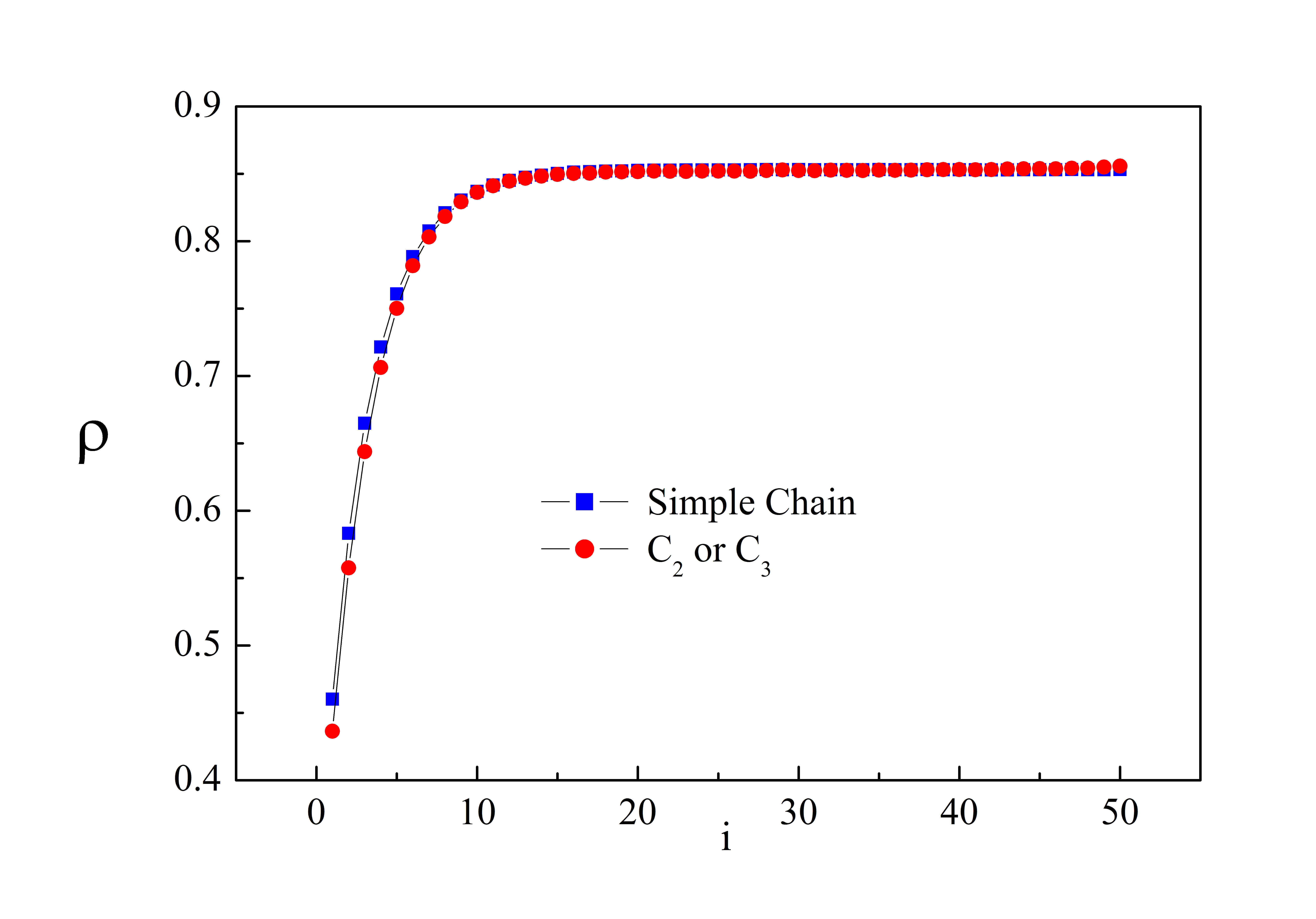
Figure 8: (Color online) Comparison of the simulation results for the particle density profile $\rho(i)$, $i=1,2,\dots,50$, in the HD phase of a chain $C_{2,3}$ in the network (shown by solid (red) circles) and an open simple chain (shown by solid (blue) squares) under the estimated rates $\alpha=0.232$ and $\beta=0.147$.

However, as in the previous case, the DW interpretation $A=\rho_{+}-\rho_{-}$ leads to $\rho_{-}\simeq 0.259$, a value which does not support the current $J^{(2,3)}=J^{max}$ and, therefore cannot describe a bulk LD phase.

IV Discussion

Non-equilibrium phenomena are much more often encountered and more diverse in nature than the true equilibrium phenomena. The development of our understanding of physics far from equilibrium is currently under way. In this respect the study of simple non-equilibrium models plays very important role. The asymmetric simple exclusion process is one of the simplest non-equilibrium models of many-particle systems with particle conserving stochastic dynamics and boundary induced phase transitions.

Here, we have reported results on a rather unexpected property of the TASEP, defined on a simple network consisting of a single chain with a double-chain insertion. In the symmetric case of equal lengths of all the segments, and at equal injection and ejection rates $\alpha=\beta>1/2$, the network has the maximum-current (MC,CL,MC) phase structure. Then, a simple translation of the double-chain section forward or backward along the single chain induces a qualitative change in the local density profiles in the parallel chains which is characteristic of a phase transition. This “position-induced phase change” is caused by the change of the effective rates $\alpha^{*}$ and $\beta^{*}$ at the two junction points of the network.

Using the continuity of the finite-size current $J_{L}$ one can determine the effective rates $\alpha^{*}$ and $\beta^{*}$ at the two ends of the loop. Our theoretical analysis, based on the results for infinitely long chains, leads to values of $\alpha^{*}$ and $\beta^{*}$ which change with the double-section position and describe well the phase changes obtained numerically in the profiles. Note, for a finite-size system the effective rates depend on the lengths of all the chains, $L_{1}$, $L_{d}$ and $L_{4}$.

Quite interestingly, upon increasing the number of parallel chains in the inserted section, provided the parallel chains are in the LD phase, the total bulk density of particles in them goes down to to the value 1/4. Indeed, in the case of $n$ parallel equivalent chains the current through each of them is $J^{max}/n=1/(4n)$. The low density phase that supports this current has a bulk density, compare with Eq. (9),

$$\rho_{-}(J^{max}/n)=\frac{1}{2}\left(1-\sqrt{1-n^{-1}}\right).$$ (34)

Therefore,

$$\lim_{n\rightarrow\infty}n\rho_{-}(J^{max}/n)=\lim_{n\rightarrow\infty}n\;\frac{1}{2}\left(1-\sqrt{1-n^{-1}}\right)=1/4.$$ (35)

At that, the total bulk density in the $n$ parallel chains, when they are in the HD phase, increases linearly with $n$

$$n\rho_{+}(J^{max}/n)=n-1/4+O(n^{-1}),\quad\mbox{as}\quad n\rightarrow\infty.$$ (36)

Another novel observation, which we cannot explain completely, concerns the validity of the DW description of the observed density profiles in the LD and HD phases of chains $C_{2,3}$. Apparently, see Figs. 5 and 7, these profiles are excellently fitted by a single exponential function, which implies the existence of a well-defined localization length. However, the value of the amplitude $A$ of the exponential function does not agree with the DW prediction $A=\rho_{+}-\rho_{-}$, where $\rho_{+}$ and $\rho_{-}$ are the bulk densities of the HD and LD phases, respectively, which support the required current $J^{max}/2$. This phenomenon cannot be attributed to correlations specific to the network under consideration, because the same conclusions hold true for the simple chains under the corresponding boundary rates.

References

References

• (1) J. Brankov, N. Pesheva, and N. Bunzarova, Phys. Rev. E 69, 066128 (2004).
• (2) E. Pronina, A.B.Kolomeisky, J. Stat. Mech.: Theory Exp., P07010 (2005).
• (3) M. Basu and P.K.Mohanty, J. Stat. Mech.: Theory Exp., P10014 (2010).
• (4) B. Embley, A. Parmeggiani, N. Kern, J. Phys.: Condens. Matter 20, 295213 (2008).
• (5) B. Embley, A. Parmeggiani, N. Kern, Phys. Rev. E 80, 041128 (2009).
• (6) R. Wang, M. Liu, and R. Jiang, Phys. Rev. E 77, 051108 (2008).
• (7) S.-W. Kim and J. D. Noh, Phys. Rev. E 80, 026119 (2009).
• (8) B. Tadić, Eur. Phys. J., B 23, 221 (2001).
• (9) R. Guimerà, A. Diaz-Guilera, F. Vega-Redondo, A. Cabrales, and A. Arenas, Phys. Rev. Lett. 89, 248701 (2002).
• (10) J.D. Noh and H. Rieger, Phys. Rev. Lett. 92, 118701 (2004).
• (11) B. Tadić and M. Mitrović, Eur. Phys. J., B 71, 631 (2009).
• (12) P. Echenique, J. Gómez-Gardeñes, and Y. Moreno, Europh. Lett., 71, 325 (2005).
• (13) I. Neri, N. Kern, and A. Parmeggiani, Phys. Rev. Lett. 107, 068702 (2011).
• (14) L. Jonathan Cook and R. K. P. Zia, J. Stat. Mech.: Theory Exp., P02012 (2009).
• (15) P. Greulich, L. Ciandrini, R. J. Allen, and M. Carmen Romano, Phys. Rev. E 85, 011142 (2012).
• (16) C. A. Brackley, L. Ciandrini, and M. Carmen Romano, J. Stat. Mech.: Theory Exp., P03002 (2012).
• (17) N. Rajewsky, L. Santen, A. Schadschneider, and M. Schreckenberg, J. Stat. Phys. 92, 151-194 (1998).
• (18) M. R. Evans, N. Rajewsky, and E. R. Speer, J. Stat. Phys. 95, 45 (1999).
• (19) G. M. Schutz, in Phase Transitions and Critical Phenomena, edited by C. Domb and J. L. Lebowitz (Academic Press, London, 2001), Vol. 19.
• (20) A. B. Kolomeisky, G. M. Sch.utz, E. B. Kolomeisky and J. P. Straley, J. Phys. A 31, 6911 (1998).
• (21) L. Santen and C. Appert, J. Stat. Phys. 106, 187 (2002).