Markov chain Monte Carlo methods for the regular two-level fractional factorial designs and cut ideals

Abstract

It is known that a Markov basis of the binary graph model of a graph $G$ corresponds to a set of binomial generators of cut ideals $I_{\widehat{G}}$ of the suspension $\widehat{G}$ of $G$. In this paper, we give another application of cut ideals to statistics. We show that a set of binomial generators of cut ideals is a Markov basis of some regular two-level fractional factorial design. As application, we give a Markov basis of degree 2 for designs defined by at most two relations.

Introduction

Application of Gröbner bases theory to designed experiments is one of the main branches in a relatively new field in statistics, called computational algebraic statistics. The first work in this branch is given by Pistone and Wynn ([20]). In this paper, they presented a method to handle fractional factorial designs algebraically by defining design ideals. As one of the merits to consider design ideals, confounding relations between the factor effects can be generalized naturally from regular to non-regular designs and can be expressed concisely by the Gröbner bases theory. See [20] or [12] for details. After this work, various algebraic techniques based on the Gröbner bases theory are applied to the problems of designed experiments both by algebraists and statisticians. For example, an indicator function defined in [11] is a valuable tool to characterize non-regular fractional factorial designs.

On the other hand, there is another main branch in the field of computational algebraic statistics. In this branch, a key notion is a Markov basis, which is defined by Diaconis and Sturmfels ([7]). In this work, they established a procedure for sampling from discrete conditional distributions by constructing a connected Markov chain on a given sample space. Since this work many papers are given considering Markov bases for various statistical models, especially for the hierarchical models of multi-dimensional contingency tables. Intensive results on the structure of Markov bases for various statistical models are given in [3].

The arguments in this paper relates to both of the two branches mentioned above. In fact, the motivation of this paper is of interest to investigate statistical problems which are related to both designed experiments and Markov bases. This paper is based on the first works with this motivation, [5] and [4]. In these works, Markov chain Monte Calro methods for testing factor effects are discussed, when observations are discrete and are given in the two-level or three-level regular fractional factorial designs. As one of the contributions of these works, the relation between the statistical models for the regular fractional factorial designs and contingency tables is considered through Markov bases. As a consequence, to investigate the Markov bases arising in the problems of designed experiments, we can refer to the known results on the corresponding models for the contingency tables. For example, we see that the Markov basis for the main effect models of the regular $2^{5-2}_{{\rm III}}$ design given by the defining relation ${\bf A}{\bf B}{\bf D}={\bf A}{\bf C}{\bf E}={\bf I}$ is constructed only by the square-free degree 2 elements ([5]). This is because the corresponding model in the contingency tables is the conditional independence model in the $2\times 2\times 2$ table. Note that the conditional independence model in the three-way contingency table is an example of decomposable models and we know the fact that a minimal Markov basis for this class of models can be constructed only by square-free degree 2 elements. See [9] for detail.

In this paper, following the Markov chain Monte Carlo approach in the designed experiments by [5] and [4], we give a new results on the correspondence between the regular two-level design and the algebraic concept, namely cut ideals defined in [21]. Because the Markov bases are characterized as the generators of well-specified toric ideals and are studied not only by statisticians but also by algebraists, it is valuable to connect statistical models to known class of toric ideals. In this paper, we give a fundamental fact that the generator of cut ideals can be characterized as the Markov bases for the testing problems of log-linear models for the two-level regular fractional factorial designs.

The construction of this paper is as follows. In Section 1 we review Markov chain Monte Carlo approach for testing the fitting of the log-linear models when observations are discrete random variables. The main results of this paper are given in Section 2. We show how to relate cut ideals to the fractional factorial designs and give the main theorem. In Section 3, we apply known results on the cut ideals to the regular fractional factorial designs.

1 Markov chain Monte Carlo method for regular two-level fractional factorial designs

In this section we introduce Markov chain Monte Carlo methods for testing the fitting of the log-linear models for regular two-level fractional factorial designs with count observations. Suppose we have nonnegative integer observations for each run of a regular fractional design. For simplicity, we also suppose that the observations are counts of some events and only one observation is obtained for each run. This is natural for the settings of Poisson sampling scheme, since the set of the totals for each run is the sufficient statistics for the parameters. We begin with an example.

Example 1.1 (Wave-soldering experiment).

Table 1 is a $1/8$ fraction of a full factorial design (i.e., a $2^{7-3}$ fractional factorial design) defined from the defining relation

$${\bf A}{\bf B}{\bf D}{\bf E}={\bf A}{\bf C}{\bf D}{\bf F}={\bf B}{\bf C}{\bf D}{\bf G}={\bf I},$$ (1)

and response data analyzed in [6] and reanalyzed in [14].

Table 1: Design and number of defects $y$ for the wave-solder experiment

	Factor							$y$
Run	${\bf A}$	${\bf B}$	${\bf C}$	${\bf D}$	${\bf E}$	${\bf F}$	${\bf G}$	1	2	3
1	1	1	1	1	1	1	1	13	30	26
2	1	1	1	2	2	2	2	4	16	11
3	1	1	2	1	1	2	2	20	15	20
4	1	1	2	2	2	1	1	42	43	64
5	1	2	1	1	2	1	2	14	15	17
6	1	2	1	2	1	2	1	10	17	16
7	1	2	2	1	2	2	1	36	29	53
8	1	2	2	2	1	1	2	5	9	16
9	2	1	1	1	2	2	1	29	0	14
10	2	1	1	2	1	1	2	10	26	9
11	2	1	2	1	2	1	2	28	173	19
12	2	1	2	2	1	2	1	100	129	151
13	2	2	1	1	1	2	2	11	15	11
14	2	2	1	2	2	1	1	17	2	17
15	2	2	2	1	1	1	1	53	70	89
16	2	2	2	2	2	2	2	23	22	7

In Table 1, the observation $y$ is the number of defects arising in a wave-soldering process in attaching components to an electronic circuit card. In Chapter 7 of [6], he considered seven factors of a wave-soldering process: (A) prebake condition, (B) flux density, (C) conveyer speed, (D) preheat condition, (E) cooling time, (F) ultrasonic solder agitator and (G) solder temperature, each at two levels with three boards from each run being assessed for defects. The aim of this experiment is to decide which levels for each factors are desirable to reduce solder defects.

Because we only consider designs with a single observation for each run in this paper, we focus on the totals for each run in Table 1. We also ignore the second observation in run 11, which is an obvious outlier as pointed out in [14]. Therefore the weighted total of run 11 is $(28+19)\times 3/2=70.5\simeq 71$. By replacing $2$ by $-1$ in Table 1, we rewrite $k\times p$ design matrix as $D$, where each element is $+1$ or $-1$. Consequently, we have

$$D=\left(\begin{array}[]{ccccccc}+1&+1&+1&+1&+1&+1&+1\\ +1&+1&+1&-1&-1&-1&-1\\ +1&+1&-1&+1&+1&-1&-1\\ +1&+1&-1&-1&-1&+1&+1\\ +1&-1&+1&+1&-1&+1&-1\\ +1&-1&+1&-1&+1&-1&+1\\ +1&-1&-1&+1&-1&-1&+1\\ +1&-1&-1&-1&+1&+1&-1\\ -1&+1&+1&+1&-1&-1&+1\\ -1&+1&+1&-1&+1&+1&-1\\ -1&+1&-1&+1&-1&+1&-1\\ -1&+1&-1&-1&+1&-1&+1\\ -1&-1&+1&+1&+1&-1&-1\\ -1&-1&+1&-1&-1&+1&+1\\ -1&-1&-1&+1&+1&+1&+1\\ -1&-1&-1&-1&-1&-1&-1\\ \end{array}\right),\ \ {\bf y}=\left(\begin{array}[]{c}69\\ 31\\ 55\\ 149\\ 46\\ 43\\ 118\\ 30\\ 43\\ 45\\ 71\\ 380\\ 37\\ 36\\ 212\\ 52\end{array}\right).$$

In this paper, we consider designs of $p$ factors with two-level. We write the observations as ${\bf y}=(y_{1},\ldots,y_{k})^{\prime}$, where $k$ is the run size and ^′ denotes the transpose. Write the design matrix $D=(d_{ij})$, where $d_{ij}\in\{-1,1\}$ is the level of the $j$-th factor in the $i$-th run for $i=1,\ldots,k,j=1,\ldots,p$.

In this case it is natural to consider the Poisson distribution as the sampling model, in the framework of generalized linear models ([17]). The observations ${\bf y}$ are realizations from $k$ Poisson random variables $Y_{1},\ldots,Y_{k}$, which are mutually independently distributed with the mean parameter $\mu_{i}=E(Y_{i}),i=1,\ldots,k$. We call the log-linear model written by

$$\log\mu_{i}=\beta_{0}+\beta_{i}d_{i1}+\cdots+\beta_{p}d_{ip},\ i=1,\ldots,k$$ (2)

as the main effect model in this paper. The equivalent model in the matrix form is

$$\left(\begin{array}[]{c}\log\mu_{1}\\ \vdots\\ \log\mu_{k}\end{array}\right)=M{\bf\beta},$$

where ${\bf\beta}=(\beta_{0},\beta_{1},\ldots,\beta_{p})^{\prime}$ and

$$M=\left(\begin{array}[]{cccc}1&&&\\ \vdots&&D&\\ 1&&&\end{array}\right).$$ (3)

We call the $k\times(p+1)$ matrix $M$ a model matrix of the main effect model. The interpretation of the parameter $\beta_{j}$ in (2) is the parameter contrast for the main effect of the $j$-th factor. Following the arguments of [5], we can also consider the models including various interaction effects. In this paper, we first describe our methods for the main effect models and will consider how to treat interaction effects afterward.

To judge the fitting of the main effect model (2), we can perform various goodness-of-fit tests. In the goodness-of-fit tests, the main effect model (2) is treated as the null model, whereas the saturated model is treated as the alternative model. Under the null model (2), ${\bf\beta}$ is the nuisance parameter and the sufficient statistic for ${\bf\beta}$ is given by $M^{\prime}{\bf y}=(\sum_{i=1}^{k}y_{i},\sum_{i=1}^{k}d_{i1}y_{i},\ldots,\allowbreak\sum_{i=1}^{k}d_{ip}y_{i})^{\prime}$. Then the conditional distribution of ${\bf y}$ given the sufficient statistics is written as

$$f({\bf y}\ |\ M^{\prime}{\bf y}=M^{\prime}{\bf y}^{o})=\frac{1}{C(M^{\prime}{\bf y}^{o})}\displaystyle\prod_{i=1}^{k}\frac{1}{y_{i}!},$$ (4)

where ${\bf y}^{o}$ is the observation count vector and $C(M^{\prime}{\bf y}^{o})$ is the normalizing constant determined from $M^{\prime}{\bf y}^{o}$ written as

$$C(M^{\prime}{\bf y}^{o})=\displaystyle\sum_{{\bf y}\in{\cal F}(M^{\prime}{\bf y}^{o})}\left(\displaystyle\prod_{i=1}^{k}\frac{1}{y_{i}!}\right),$$ (5)

and

$${\cal F}(M^{\prime}{\bf y}^{o})=\{{\bf y}\ |\ M^{\prime}{\bf y}=M^{\prime}{\bf y}^{o},\ y_{i}\ \mbox{is a nonnegative integer for}\ i=1,\ldots,k\}.$$ (6)

Note that by sufficiency the conditional distribution does not depend on the values of the nuisance parameters.

In this paper we consider various goodness-of-fit tests based on the conditional distribution (4). There are several ways to choose the test statistics. For example, the likelihood ratio statistic

$$T({\bf y})=G^{2}({\bf y})=2\sum_{i=1}^{k}y_{i}\log\frac{y_{i}}{\hat{\mu_{i}}}$$ (7)

is frequently used, where $\hat{\mu_{i}}$ is the maximum likelihood estimate for $\mu_{i}$ under the null model (i.e., fitted value). Note that the traditional asymptotic test evaluates the upper probability for the observed value $T({\bf y}^{o})$ based on the asymptotic distribution $\chi_{k-p-1}^{2}$. However, since the fitting of the asymptotic approximation may be sometimes poor, we consider Markov chain Monte Carlo methods to evaluate the $p$ values. Using the conditional distribution (4), the exact $p$ value is written as

$$p=\displaystyle\sum_{{\bf y}\in{\cal F}(M^{\prime}{\bf y}^{o})}f({\bf y}\ |\ M^{\prime}{\bf y}=M^{\prime}{\bf y}^{o}){\bf 1}(T({\bf y})\geq T({\bf y}^{o})),$$ (8)

where

$${\bf 1}(T({\bf y})\geq T({\bf y}^{o}))=\left\{\begin{array}[]{ll}1,&\mbox{if}\ T({\bf y})\geq T({\bf y}^{o}),\\ 0,&\mbox{otherwise}.\end{array}\right.$$ (9)

Of course, if we can calculate the exact $p$ value of (8) and (9), it is best. Unfortunately, however, an enumeration of all the elements in ${\cal F}(M^{\prime}{\bf y}^{o})$ and hence the calculation of the normalizing constant $C(M^{\prime}{\bf y}^{o})$ is usually computationally infeasible for large sample space. Instead, we consider a Markov chain Monte Carlo method. Note that, as one of the important advantages of Markov chain Monte Carlo method, we need not calculate the normalizing constant (5) to evaluate $p$ values.

To perform the Markov chain Monte Carlo procedure, we have to construct a connected, aperiodic and reversible Markov chain over the conditional sample space (6) with the stationary distribution (4). If such a chain is constructed, we can sample from the chain as ${\bf y}^{(1)},\ldots,{\bf y}^{(T)}$ after discarding some initial burn-in steps, and evaluate $p$ values as

$$\hat{p}=\frac{1}{T}\sum_{t=1}^{T}{\bf 1}(T({\bf y}^{(t)})\geq T({\bf y}^{o})).$$

Such a chain can be constructed easily by Markov basis. Once a Markov basis is calculated, we can construct a connected, aperiodic and reversible Markov chain over the space (6), which can be modified so that the stationary distribution is the conditional distribution (4) by the Metropolis-Hastings procedure. See [7] and [15] for details.

Markov basis is characterized algebraically as follows. Write indeterminates $x_{1},\ldots,x_{k}$ and consider polynomial ring $K[x_{1},\ldots,x_{k}]$ for some field $K$. Consider the integer kernel of the transpose of the model matrix $M$, ${\rm Ker}_{\mathbb{Z}}M^{\prime}$. For each ${\bf b}=(b_{1},\ldots,b_{k})^{\prime}\in{\rm Ker}_{\mathbb{Z}}M^{\prime}$, define binomial in $K[x_{1},\ldots,x_{k}]$ as

$$f_{{\bf b}}=\prod_{b_{j}>0}x_{j}^{b_{j}}-\prod_{b_{j}<0}x_{j}^{-b_{j}}.$$

Then the binomial ideal in $K[x_{1},\ldots,x_{k}]$,

$$I(M^{\prime})=\left<\{f_{{\bf b}}\ |\ {\bf b}\in{\rm Ker}_{\mathbb{Z}}M^{\prime}\}\right>,$$

is called a toric ideal with the configuration $M^{\prime}$. Let $\{f_{{\bf b}^{(1)}},\ldots,f_{{\bf b}^{(s)}}\}$ be any generating set of $I(M^{\prime})$. Then the set of integer vectors $\{{\bf b}^{(1)},\ldots,{\bf b}^{(s)}\}$ constitutes a Markov basis. See [7] for detail. To compute a Markov basis for given configuration $M^{\prime}$, we can rely on various algebraic softwares such as 4ti2 ([1]). See the following example.

Example 1.2 (Wave-soldering experiment, continued).

We analyze the data in Table 1. The fitted value under the main effect model is calculated as

$$\begin{array}[]{l}\hat{\mu}=(68.87,\ 19.70,\ 78.85,\ 147.59,\ 12.14,\ 54.77,\ 104.53,\ 54.54,\\ \hskip 28.45274pt75.31,\ 39.29,\ 75.00,\ 338.37,\ 27.83,\ 52.09,\ 208.47,\ 59.64)^{\prime}.\end{array}$$

Then the likelihood ratio for the observed data is calculated as $T({\bf y}^{o})=G^{2}({\bf y}^{o})=117.81$ and the corresponding asymptotic $p$ value is less than $0.0001$ from the asymptotic distribution $\chi_{8}^{2}$. This result tells us that the null hypothesis is highly significant and is rejected, i.e., the existence of some interaction effects is suggested. To evaluate the $p$ value by Markov chain Monte Carlo method, we have to calculate a Markov basis first. If we use 4ti2, we prepare the data file (configuration $M^{\prime}$) as

8 16
 1  1  1  1  1  1  1  1  1  1  1  1  1  1  1  1
 1  1  1  1  1  1  1  1 -1 -1 -1 -1 -1 -1 -1 -1
 1  1  1  1 -1 -1 -1 -1  1  1  1  1 -1 -1 -1 -1
 1  1 -1 -1  1  1 -1 -1  1  1 -1 -1  1  1 -1 -1
 1 -1  1 -1  1 -1  1 -1  1 -1  1 -1  1 -1  1 -1
 1 -1  1 -1 -1  1 -1  1 -1  1 -1  1  1 -1  1 -1
 1 -1 -1  1  1 -1 -1  1 -1  1  1 -1 -1  1  1 -1
 1 -1 -1  1 -1  1  1 -1  1 -1 -1  1 -1  1  1 -1

and run the command markov. Then we have a minimal Markov basis with $77$ elements as follows.

77 16
 0  0  0  0  0  0  0  0  1  1 -1 -1 -1 -1  1  1
 0  0  0  0  0  1 -1  0  1  0  0 -1 -1 -1  1  1
 0  0  0  0  0  1  0 -1  0  1  0 -1 -1 -1  1  1
 0  0  0  0  1  0 -1  0  1  0 -1  0 -1 -1  1  1
 0  0  0  0  1  0  0 -1  0  1 -1  0 -1 -1  1  1
 0  0  0  0  1  1 -1 -1  0  0  0  0 -1 -1  1  1
 0  0  0  1  0  0 -1  0  1  0 -1 -1  0 -1  1  1
.....

Using this Markov basis, we can evaluate $p$ value by Markov chain Monte Carlo method. After $50,000$ burn-in-steps from ${\bf y}^{o}$ itself as the initial state, we sample $100,000$ Monte Carlo sample by Metropolis-Hasting algorithm, which yields $\hat{p}=0.0000$ again. Figure 1 is a histogram of the Monte Carlo sampling of the likelihood ratio statistic under the main effect model, along with the corresponding asymptotic distribution $\chi^{2}_{8}$.

Figure 1: Asymptotic and Monte Carlo estimated distribution of likelihood ratio

If the fitting of the main effect model is poor, or we have some prior knowledge on the existence of interaction effects, we consider the models including interaction effects. The models including the interaction effects are also described by the model matrix. The modeling method presented in [5] is as follows. If we want to consider the models including interaction effects, add columns to the model matrix of the main effect model (3) so that the corresponding parameter can be interpreted as the parameter contrast for the additional interaction effect. We describe this point by the previous example. See [5] for details.

Example 1.3 (Wave-soldering experiment, continued).

As is pointed out in [14], the existence of some interaction effects is suggested for the data in Table 1. In [14], the model including $2$ two-factor interaction effects, ${\bf A}\times{\bf C}$ and ${\bf B}\times{\bf D}$ is considered. Here we call this model as $M_{2}$ model. The model matrix of the $M_{2}$ model is constructed by adding two columns,

$$\left(\begin{array}[]{rrrrrrrrrrrrrrrr}1&1&-1&-1&1&1&-1&-1&-1&-1&1&1&-1&-1&1&1\\ 1&-1&1&-1&-1&1&-1&1&1&-1&1&-1&-1&1&-1&1\end{array}\right)^{\prime}$$

to the model matrix of the main effect model. Note that the above two columns are the element-wise product of the (first, third) columns and the (second, fourth) columns of $D$, respectively. Using this model matrix (or configuration matrix as its transpose), we can investigate the fitting of the $M_{2}$ model in the similar way. The fitted value under the $M_{2}$ model is

$$\begin{array}[]{l}\hat{\mu}=(64.53,\ 47.25,\ 53.15,\ 151.08,\ 30.43,\ 46.79,\ 115.24,\ 32.53,\\ \hskip 28.45274pt49.42,\ 46.13,\ 70.90,\ 360.54,\ 35.19,\ 30.26,\ 232.14,\ 51.42)^{\prime}.\end{array}$$

Then the likelihood ratio for the observed data is calculated as $T({\bf y}^{o})=G^{2}({\bf y}^{o})=19.0927$ and the corresponding asymptotic $p$ value is $0.00401$ from the asymptotic distribution $\chi_{6}^{2}$. Though this result still suggests the significantly poor fitting of the $M_{2}$ model, much larger $p$ value and much smaller likelihood ratio than those of the main effect model tell us that $M_{2}$ model is much better than the main effect model. We have the Markov chain Monte Carlo estimate of $p$ value as $\hat{p}=0.0031$ from $100,000$ Monte Calro sample after $50,000$ burn-in-steps.

An important point here is that the model matrix for the models with interaction effects constructed in this way is equivalent to the model matrix for the main effect model for some regular fractional factorial design of resolution III or more. For example, the model matrix for the $M_{2}$ model in Example 1.3 is equivalent to the main effect model for the $2^{9-5}$ fractional factorial design defined from

$${\bf A}{\bf B}{\bf D}{\bf E}={\bf A}{\bf C}{\bf D}{\bf F}={\bf B}{\bf C}{\bf D}{\bf G}={\bf A}{\bf C}{\bf H}={\bf B}{\bf D}{\bf J}={\bf I}.$$

This relation is given by adding ${\bf H}={\bf A}{\bf C}$ and ${\bf J}={\bf B}{\bf D}$ to (1), as if there exists two additional factors ${\bf H}$ and ${\bf J}$ in Table 1. In this paper, we consider the relation between the model matrix and the cut ideals. From the above considerations, we can restrict our attentions to the main effect models to consider the relations to the cut ideals. We give the relation in Section 2.2. We will consider the models including interaction effects again in Section 2.3 to consider the relation from the practical viewpoint.

2 Two-level regular fractional factorial designs and cut ideals

In this section, we show that a cut ideal for a finite connected graph can be characterized as the toric ideal $I(M^{\prime})$ for a model matrix of the main effect model for some regular two-level fractional factorial designs.

2.1 Cut ideals

We start with the definition of the cut ideal. Consider a connected finite graph $G=(V,E)$. We also consider unordered partitions $A|B$ of the vertex set $V$. Let ${\cal P}(V)$ be the set of the unordered partitions of $V$, i.e.,

$${\cal P}(V)=\{A|B\ |\ A\cup B=V,\ A\cap B=\emptyset\}.$$

We introduce the sets of indeterminates $\{s_{ij}\ |\ \{i,j\}\in E\}$, $\{t_{ij}\ |\{i,j\}\in E\}$ and $\{q_{A|B}\ |\ A|B\in{\cal P}(V)\}$. Let

$$K[{\bf q}]=K[q_{A|B}\ |\ A|B\in{\cal P}(V)],$$

$$K[{\bf s},{\bf t}]=K[s_{ij},t_{ij}\ |\ \{i,j\}\in E]$$

be polynomial rings over a field $K$. For each partition $A|B\in{\cal P}(V)$, we define a subset ${\rm Cut}(A|B)$ of the edge set $E$ as

$${\rm Cut}(A|B)=\{\{i,j\}\in E\ |\ i\in A,j\in B\ {\rm or}\ i\in B,j\in A\}.$$

Define homomorphism of polynomial rings as

$$\phi_{G}:\ K[{\bf q}]\rightarrow K[{\bf s},{\bf t}],\ \ q_{A|B}\mapsto\prod_{\{i,j\}\in{\rm Cut}(A|B)}s_{ij}\ \cdot\prod_{\{i,j\}\in E\setminus{\rm Cut}(A|B)}t_{ij}.$$ (10)

We may think of ${\bf s}$ and ${\bf t}$ as abbreviations for “separated” and “together”, respectively. Then the cut ideal of the graph $G$ is defined as $I_{G}={\rm Ker}(\phi_{G})$. We also use the following two examples given in [21].

Example 2.1 (Complete graph on four vertices).

Let $G=K_{4}$ be the complete graph on four vertices $V=\{1,2,3,4\}$. Then the edge set is $E=\{12,13,14,23,24,34\}$. The map $\phi_{K_{4}}$ is specified by

$$\begin{array}[]{rcl}q_{\emptyset|1234}&\mapsto&t_{12}t_{13}t_{14}t_{23}t_{24}t_{34}\\ q_{1|234}&\mapsto&s_{12}s_{13}s_{14}t_{23}t_{24}t_{34}\\ q_{2|134}&\mapsto&s_{12}t_{13}t_{14}s_{23}s_{24}t_{34}\\ q_{3|124}&\mapsto&t_{12}s_{13}t_{14}s_{23}t_{24}s_{34}\\ q_{4|123}&\mapsto&t_{12}t_{13}s_{14}t_{23}s_{24}s_{34}\\ q_{12|34}&\mapsto&t_{12}s_{13}s_{14}s_{23}s_{24}t_{34}\\ q_{13|24}&\mapsto&s_{12}t_{13}s_{14}s_{23}t_{24}s_{34}\\ q_{14|23}&\mapsto&s_{12}s_{13}t_{14}t_{23}s_{24}s_{34}.\end{array}$$

In this case, the cut ideal is a principal ideal given by

$$I_{K_{4}}=\left<q_{\emptyset|1234}q_{12|34}q_{13|24}q_{14|23}-q_{1|234}q_{2|134}q_{3|124}q_{4|123}\right>.$$

Example 2.2 ($4$-cycle).

Let $G=C_{4}$ be the $4$-cycle with

$$V=\{1,2,3,4\},\ E=\{12,23,34,14\}.$$

The map $\phi_{C_{4}}$ is derived from $\phi_{K_{4}}$ in Example 2.1 by setting

$$s_{13}=t_{13}=s_{24}=t_{24}=1$$

as

$$\begin{array}[]{rcl}q_{\emptyset|1234}&\mapsto&t_{12}t_{14}t_{23}t_{34}\\ q_{1|234}&\mapsto&s_{12}s_{14}t_{23}t_{34}\\ q_{2|134}&\mapsto&s_{12}t_{14}s_{23}t_{34}\\ q_{3|124}&\mapsto&t_{12}t_{14}s_{23}s_{34}\\ q_{4|123}&\mapsto&t_{12}s_{14}t_{23}s_{34}\\ q_{12|34}&\mapsto&t_{12}s_{14}s_{23}t_{34}\\ q_{13|24}&\mapsto&s_{12}s_{14}s_{23}s_{34}\\ q_{14|23}&\mapsto&s_{12}t_{14}t_{23}s_{34}.\end{array}$$

In this case, the cut ideal is given by

$$I_{C_{4}}=\left<q_{\emptyset|1234}q_{13|24}-q_{1|234}q_{3|124},\ q_{\emptyset|1234}q_{13|24}-q_{2|134}q_{4|123},\ q_{\emptyset|1234}q_{13|24}-q_{12|34}q_{14|23}\right>.$$

Now we relates the cut ideals to the regular two-level fractional factorial designs. We express the map $\phi_{G}$ by $2^{|V|-1}\times 2|E|$ matrix $H=\{h_{A|B,e}\}$ where each row of $H$ represents $A|B\in{\cal P}(V)$ and each two columns of $H$ represents $E$ as

$$h_{A|B,e}=\left\{\begin{array}[]{ll}(1,0)&\mbox{if}\ e\in E\setminus{\rm Cut}(A|B)\\ (0,1)&\mbox{if}\ e\in{\rm Cut}(A|B).\end{array}\right.$$

Note that there are $|{\cal P}(V)|=2^{|V|-1}$ unordered partitions of $V$. We also see that each two columns of $H$ correspond to ${\bf t}$ and ${\bf s}$. Then the cut ideal, the kernel of $\phi_{G}$ of (10), is written as the toric ideal of the configuration matrix $H^{\prime}$.

Example 2.3 ($4$-cycle, continued).

For the case of $G=C_{4}$ of Example 2.2, the matrix $H$ can be written as follows.

$$\begin{array}[]{c|cccccccc|}\lx@intercol\hfil\hfil\lx@intercol&t_{12}&s_{12}&t_{14}&s_{14}&t_{23}&s_{23}&t_{34}&\lx@intercol\hfil s_{34}\hfil\lx@intercol\\ \cline{2-9}\cr q_{\emptyset|1234}&1&0&1&0&1&0&1&0\\ q_{3|124}&1&0&1&0&0&1&0&1\\ q_{4|123}&1&0&0&1&1&0&0&1\\ q_{12|34}&1&0&0&1&0&1&1&0\\ q_{14|23}&0&1&1&0&1&0&0&1\\ q_{2|134}&0&1&1&0&0&1&1&0\\ q_{1|234}&0&1&0&1&1&0&1&0\\ q_{13|24}&0&1&0&1&0&1&0&1\\ \cline{2-9}\cr\end{array}$$ (11)

The kernel of $H^{\prime}$ coincides to the kernel of $M^{\prime}$ of (3) for the two-level design $D$ of $|E|$ factors with $2^{|V|-1}$ runs, where the level of the factor $X_{e}$ for the run $A|B\in{\cal P}(V)$ is given by the following map:

$$\begin{array}[]{cccc}X_{e}:&{\cal P}(V)&\rightarrow&\{+1,-1\}\\ &\rotatebox{90.0}{$\in$}&&\rotatebox{90.0}{$\in$}\\ &A|B&\mapsto&\left\{\begin{array}[]{ll}+1&\mbox{if}\ e\in E\setminus{\rm Cut}(A|B)\\ -1&\mbox{if}\ e\in{\rm Cut}(A|B)\end{array}\right.\end{array}$$ (12)

Example 2.4 ($4$-cycle, continued).

For the case of $G=C_{4}$, the map $X_{e}$ of (12) gives the design matrix $D$ as follows.

$$\begin{array}[]{c|rrrr|}\lx@intercol\hfil\hfil\lx@intercol&X_{12}&X_{14}&X_{23}&\lx@intercol\hfil X_{34}\hfil\lx@intercol\\ \cline{2-5}\cr q_{\emptyset|1234}&1&1&1&1\\ q_{3|124}&1&1&-1&-1\\ q_{4|123}&1&-1&1&-1\\ q_{12|34}&1&-1&-1&1\\ q_{14|23}&-1&1&1&-1\\ q_{2|134}&-1&1&-1&1\\ q_{1|234}&-1&-1&1&1\\ q_{13|24}&-1&-1&-1&-1\\ \cline{2-5}\cr\end{array}$$

For this $D$, it is easily seen that ${\rm Ker}(M^{\prime})$ coincides to ${\rm Ker}(H^{\prime})$ if $H$ is given by (11).

2.2 Regular designs and cut ideals

In Example 2.4, we obtain the toric ideal for the main effect model of the regular two-level fractional factorial designs defined by $X_{12}X_{14}X_{23}X_{34}=1$ from the the cut ideal of $G=C_{4}$. In fact, there is a clear relation between finite connected graphs $G$ and regular two-level designs $D$. As we have seen in Example 2.4, the cut ideal for $G$ can be related to the design of $p=|E|$ factors with $k=2^{|V|-1}$ runs. Since each factor of this design corresponds to the edge $E$ of $G$, we write each factor $X_{ij}$ for $\{i,j\}\in E$. Since there are $2^{p}$ runs in the full factorial design of $p$ factors, the design obtained from $G$ by the relation (12) is a $2^{|V|-1-p}$ fraction of the full factorial design of $p$ factors. We show this fraction is specified as the regular fractional factorial designs.

Let $G=(V,E)$ be a finite connected graph with the edge set $E=\{e_{1},\ldots,e_{p}\}$. Then, the cycle space $\mathcal{C}(G)$ of $G$ is a subspace of $\mathbb{F}_{2}^{|E|}$ spanned by

$$\left\{\left.{\bf e}_{i_{1}}+\cdots+{\bf e}_{i_{r}}\in\mathbb{F}_{2}^{|E|}\ \right|\ (e_{i_{1}},\ldots,e_{i_{r}})\mbox{ is a cycle of }G\right\},$$

where ${\bf e}_{j}$ is the $j$th coordinate vector of $\mathbb{F}_{2}^{|E|}$. On the other hand, the cut space $\mathcal{C}^{*}(G)$ of $G$ is a subspace of $\mathbb{F}_{2}^{|E|}$ defined by

$$\mathcal{C}^{*}(G)=\left\{\left.\sum_{e_{j}\in{\rm Cut}(A|B)}{\bf e}_{j}\in\mathbb{F}_{2}^{|E|}\ \right|\ A|B\in\mathcal{P}(V)\right\}.$$

Fix a spanning tree $T$ of $G$. For each $e\in E\setminus T$, the set $T\cup\{e\}$ has exactly one cycle $C_{e}$ of $G$. Such a cycle $C_{e}$ is called a fundamental cycle of $G$. Since $T$ has $|V|-1$ edges, there are $|E|-|V|+1$ edges in $E\setminus T$. It then follows that there exists $|E|-|V|+1$ fundamental cycles in $G$. The following proposition is known in graph theory [8]:

Proposition 2.5.

Let $G=(V,E)$ be a finite connected graph. Then, we have the following:

• $\mathcal{C}^{*}(G)=\mathcal{C}(G)^{\perp}\left(=\left\{\left.{\bf v}\in\mathbb{F}_{2}^{|E|}\ \right|\ {\bf v}\cdot{\bf u}=0\mbox{ for all }{\bf u}\in\mathcal{C}(G)\right\}\right);$

• Given spanning tree of $G$, the cycle space $\mathcal{C}(G)$ is spanned by

  $$\left\{\left.{\bf e}_{i_{1}}+\cdots+{\bf e}_{i_{r}}\in\mathbb{F}_{2}^{|E|}\ \right|\ (e_{i_{1}},\ldots,e_{i_{r}})\mbox{ is a fundamental cycle of }G\right\};$$

• $\dim\mathcal{C}(G)=|E|-|V|+1$ and $\dim\mathcal{C}^{*}(G)=|V|-1$.

By Proposition 2.5, we have the following:

Theorem 2.6.

Let $G=(V,E)$ be a finite connected graph and let $D$ be the design matrix of $|E|$ factors with $2^{|V|-1}$ runs defined by (12). Then $D$ is a regular fractional factorial design with all relations

$$X_{e_{i_{1}}}(A|B)X_{e_{i_{2}}}(A|B)\cdots X_{e_{i_{m}}}(A|B)=1,$$ (13)

where $(e_{i_{1}},\ldots,e_{i_{m}})$ is a fundamental cycle of $G$.

Proof.

The equation (13) is equivalent to the equation

$$({\bf e}_{i_{1}}+\cdots+{\bf e}_{i_{m}})\cdot\left(\sum_{e_{j}\in{\rm Cut}(A|B)}{\bf e}_{j}\right)=0$$

in $\mathbb{F}_{2}^{|E|}$. Thus, the assertion follows from (i) and (ii) of Proposition 2.5. ∎

It may be a helpful to see a typical example.

Example 2.7.

Consider $G=(V,E)$ given by

$$V=\{1,2,3,4,5,6\},\ E=\{12,13,23,34,45,56,26\}.$$

From (13), we see that $G$ corresponds to $2^{7-3}$ design with

$$X_{12}X_{13}X_{23}=X_{13}X_{34}X_{45}X_{15}=X_{12}X_{26}X_{56}X_{15}=1.$$

Note that the relations corresponding the dependent cycles such as $\{23,34,45,56,26\}$ can be derived as

$$X_{23}X_{34}X_{45}X_{56}X_{26}=(X_{12}X_{13}X_{23})(X_{13}X_{34}X_{45}X_{15})(X_{12}X_{26}X_{56}X_{15})=1.$$

Theorem 2.6 shows the relation of the cut ideals and regular two-level fractional factorial designs. For a given connected finite graph, we can consider corresponding regular two-level fractional factorial designs from Theorem 2.6. Unfortunately, however, the converse does not always hold. For given regular two-level fractional factorial designs (strictly, we should say that “for given designs and models”, which we consider in Section 2.3), it does not always exist corresponding connected finite graphs.

Proposition 2.8.

If a $2^{p-q}$ design corresponds to a finite graph by the relation (12), then we have $p\leq{p-q+1\choose{2}}$.

Proof.

Corresponding connected graphs $G=(V,E)$ does not exist because $|E|=p$ and $|V|=p-q+1$ must be satisfied if it exists. (There are ${p-q+1\choose{2}}$ edges in $K_{p-q+1}$.) ∎

Thus, obvious counterexamples for the converse are given since some regular $2^{p-q}$ designs satisfy ${p-q+1\choose{2}}<p$ (for example, $(p,q)=(5,3),(5,4),(6,4),(6,5)$ and so on). On the other hand, a necessary condition related with the resolution is as follows.

Proposition 2.9.

If a $2^{p-q}$ design of resolution ${\rm IV}$ or more corresponds to a finite graph by the relation (12), then we have $p\leq\lfloor(p-q+1)^{2}/4\rfloor$.

Proof.

Mantel’s theorem in graph theory says that the number of edges in triangle-free graph with $n$ vertices is at most $\lfloor n^{2}/4\rfloor$. ∎

If the resolution of a design is ${\rm V}$ or more, then similar results are obtained by the results in [13]. From these considerations, an important question arises.

Question 2.10.

Characterize regular two-level fractional factorial designs that can correspond to a finite graph by the relation (12).

A complete answer to this question is not yet obtained at present. We give results for $8$ runs and $16$ runs designs in Section 2.3. We present several fundamental characterizations in the rest of this section. Note that the above correspondence is not one-to-one even if it exists. In fact, for any finite connected graph $G$, we can specify a design $D$ uniquely by (13). However, for a given design $G$, we can consider several graphs satisfying the relation (13) if it exists.

Example 2.11 ($2^{5-1}$ design with $X_{12}X_{13}X_{23}=1$ of $5$ factors).

Consider $2^{5-1}$ fractional factorial design $X_{12}X_{13}X_{23}=1$ of $5$ factors, or, ${\bf A}{\bf B}{\bf C}={\bf I}$ in the convention of designed experiment literature. There are several corresponding graphs that give this design such as follows.

Later, we will be able to understand this by Proposition 3.1. (Both of two graphs are 0-sum of the same pair of graphs.)

Now we show two important special cases, designs corresponding to complete graphs and trees.

Example 2.12 (Complete graph on four vertices (continued)).

Let $G=K_{4}$ be the complete graph on four vertices $V=\{1,2,3,4\}$ in Example 2.1.

From (13), we have the following regular $2^{6-3}$ fractional factorial design.

$$\begin{array}[]{c|rrrrrr|}\lx@intercol\hfil\hfil\lx@intercol&X_{12}&X_{13}&X_{14}&X_{23}&X_{24}&\lx@intercol\hfil X_{34}\hfil\lx@intercol\\ \cline{2-7}\cr q_{\emptyset|1234}&1&1&1&1&1&1\\ q_{3|124}&1&-1&1&-1&1&-1\\ q_{4|123}&1&1&-1&1&-1&-1\\ q_{12|34}&1&-1&-1&-1&-1&1\\ q_{14|23}&-1&-1&1&1&-1&-1\\ q_{2|134}&-1&1&1&-1&-1&1\\ q_{1|234}&-1&-1&-1&1&1&1\\ q_{13|24}&-1&1&-1&-1&1&-1\\ \cline{2-7}\cr\end{array}$$

The defining relation of this design is

$$X_{12}X_{13}X_{23}=X_{12}X_{14}X_{24}=X_{13}X_{14}X_{34}=1,$$

where the three terms $X_{12}X_{13}X_{23},X_{12}X_{14}X_{24},X_{13}X_{14}X_{34}$ correspond to the independent cycle of $K_{4}$.

Generalizing Example 2.12, we summarize the following important cases.

Corollary 2.13.

Let $G=K_{n}$ be the complete graph on $|V|=n$ vertices. Then, $G$ is specified as the regular $2^{c_{1}-c_{2}}$ fractional factorial design of $c_{1}$ two-level factors by (13), where

$$c_{1}={n\choose{2}},\ \ c_{2}={n-1\choose{2}}.$$

The defining relation of this design is written as $X_{1i}X_{1j}X_{ij}=1$ for any pair $(i,j)$ with $2\leq i<j\leq n$.

Another important case is as follows.

Corollary 2.14.

Any spanning tree $G=(V,E)$ is specified as the full factorial design of $|V|-1$ two-level factors by (13).

2.3 Models for the designs with $8$ runs and $16$ runs

It seems very difficult to answer Question 2.10 in general. As special cases, we show that $2^{p-1}$ and $2^{p-2}$ fractional factorial designs can relate to graphs from algebraic theories in Section 3. As another approach, we investigate all the practical models arising in the two-level fractional factorial designs with $8$ runs and $16$ runs. In Section 2.3, we consider models with interaction effects to classify the cases arising in applications.

First we consider models for the designs with $8$ runs. Among the regular designs with $8$ runs, the most frequently used designs are listed in Table 2.

Table 2: $2^{p-q}$ fractional factorial designs with $8$ runs ($p-q=3$)

Number of factors $p$	Resolution	Design Generators
4	IV	${\bf D}={\bf A}{\bf B}{\bf C}$
5	III	${\bf D}={\bf A}{\bf B},\ {\bf E}={\bf A}{\bf C}$
6	III	${\bf D}={\bf A}{\bf B},\ {\bf E}={\bf A}{\bf C},\ {\bf F}={\bf B}{\bf C}$
7	III	${\bf D}={\bf A}{\bf B},\ {\bf E}={\bf A}{\bf C},\ {\bf F}={\bf B}{\bf C},{\bf G}={\bf A}{\bf B}{\bf C}$

We ignore $2^{7-4}_{{\rm III}}$ design in Table 2 since the main effect model is saturated and cannot be tested in our method. For the other $3$ designs, $2^{4-1}_{\rm IV},2^{5-2}_{\rm III}$ and $2^{6-3}_{\rm III}$ designs, we consider models to be tested.

For $2^{4-1}_{\rm IV}$ design of ${\bf A}{\bf B}{\bf C}{\bf D}={\bf I}$, we can consider $3$ models as follows.

• Main effect model:
  We write it as ${\bf A}/{\bf B}/{\bf C}/{\bf D}$.

• Models with all the main effects and $1$ two-factor interaction effect:
  Without loss of generality, we consider ${\bf A}\times{\bf B}$ as the interaction effect. We write it as ${\bf A}{\bf B}/{\bf C}/{\bf D}$.

• Models with all the main effects and $2$ two-factor interaction effects:
  Note that we cannot consider models including, say, ${\bf A}\times{\bf B}$ and ${\bf C}\times{\bf D}$, because they are confounded. Without loss of generality, we consider ${\bf A}\times{\bf B}$ and ${\bf A}\times{\bf C}$ as the two interaction effects. We write it as ${\bf A}{\bf B}/{\bf A}{\bf C}/{\bf D}$.

Note that we cannot consider models with more than $2$ two-factor interactions because there are $8$ parameters in the saturated models for the design with $8$ runs. For these models, we can construct model matrix and consider existence of corresponding graphs. As we have seen, the model ${\bf A}/{\bf B}/{\bf C}/{\bf D}$ can relate to the $4$-cycle. For the model ${\bf A}{\bf B}/{\bf C}/{\bf D}$, we introduce imaginary factor ${\bf E}={\bf A}{\bf B}$ and consider the main effect model for the $2^{5-2}$ design defined by

$${\bf A}{\bf B}{\bf C}{\bf D}={\bf A}{\bf B}{\bf E}\ (={\bf C}{\bf D}{\bf E})={\bf I}$$

as we have seen in the last of Section 1. This corresponds to the graph with $5$ edges as follows.

Similarly, for the model ${\bf A}{\bf B}/{\bf A}{\bf C}/{\bf D}$, introducing imaginary factors ${\bf E}={\bf A}{\bf B}$ and ${\bf F}={\bf A}{\bf C}$ and consider the main effect model for the $2^{6-3}$ design defined by

$${\bf A}{\bf B}{\bf C}{\bf D}={\bf A}{\bf B}{\bf E}={\bf A}{\bf C}{\bf F}={\bf I},$$

we see the corresponding graph is $K_{4}$.

For $2^{5-2}_{\rm III}$ design of ${\bf D}={\bf A}{\bf B},{\bf E}={\bf A}{\bf C}$, we can consider only one additional interaction effect to the main effect model. Therefore there are the following $2$ models to be considered.

• Main effect model:
  We write it as ${\bf A}/{\bf B}/{\bf C}/{\bf D}/{\bf E}$.

• Models with all the main effects and $1$ two-factor interaction effect:
  Note that we cannot consider models including, say, ${\bf A}\times{\bf B}$, because it is confounded to the main effect of ${\bf D}$. Without loss of generality, we consider ${\bf B}\times{\bf C}$ as the interaction effect, with we write ${\bf A}/{\bf B}{\bf C}/{\bf D}/{\bf E}$.

For these models, we can construct model matrix and consider existence of corresponding graphs. The model ${\bf A}/{\bf B}/{\bf C}/{\bf D}/{\bf E}$ can relate to the graph as follows.

We see the model ${\bf A}/{\bf B}{\bf C}/{\bf D}/{\bf E}$ can relate to $K_{4}$ by introducing imaginary factor ${\bf F}={\bf B}{\bf C}$.

Finally, for $2^{6-3}_{\rm III}$ design of ${\bf D}={\bf A}{\bf B},{\bf E}={\bf A}{\bf C},{\bf F}={\bf B}{\bf C}$, only the main effect model can be considered, which can be relate to $K_{4}$.

From the above considerations, we have complete classification of all the hierarchical models for the designs with $8$ runs in Table 2. We summarize the results in Table 3 and Table 4.

Table 3: Models for the designs in Table 2

Design	Num. of parameters	Model	Index
$2^{4-1}_{\rm IV}$	$5$	${\bf A}/{\bf B}/{\bf C}/{\bf D}$	[1]
	$6$	${\bf A}{\bf B}/{\bf C}/{\bf D}$	[2]
	$7$	${\bf A}{\bf B}/{\bf A}{\bf C}/{\bf D}$	[3]
$2^{5-2}_{\rm III}$	$6$	${\bf A}/{\bf B}/{\bf C}/{\bf D}/{\bf E}$	[4]
	$7$	${\bf A}/{\bf B}{\bf C}/{\bf D}/{\bf E}$	[5]
$2^{6-3}_{\rm III}$	$7$	${\bf A}/{\bf B}/{\bf C}/{\bf D}/{\bf E}/{\bf F}$	[6]

Table 4: Graphs corresponding to the models in Table 3

Graph	Models
	[1]
	[2][4]
	[3][5][6]

Next we consider models for the designs with $16$ runs in a similar way. The most frequently used designs with $16$ runs are given Section 4 of [22], which we show in Table 5.

Table 5: $2^{p-q}$ fractional factorial designs with $16$ runs ($p-q=4$)

Number of factors $p$	Resolution	Design Generators
5	V	${\bf E}={\bf A}{\bf B}{\bf C}{\bf D}$
6	IV	${\bf E}={\bf A}{\bf B}{\bf C},{\bf F}={\bf A}{\bf B}{\bf D}$
7	IV	${\bf E}={\bf A}{\bf B}{\bf C},{\bf F}={\bf A}{\bf B}{\bf D},{\bf G}={\bf A}{\bf C}{\bf D}$
8	IV	${\bf E}={\bf A}{\bf B}{\bf C},{\bf F}={\bf A}{\bf B}{\bf D},{\bf G}={\bf A}{\bf C}{\bf D}$
		${\bf H}={\bf B}{\bf C}{\bf D}$
9	III	${\bf E}={\bf A}{\bf B}{\bf C},{\bf F}={\bf A}{\bf B}{\bf D},{\bf G}={\bf A}{\bf C}{\bf D}$
		${\bf H}={\bf B}{\bf C}{\bf D},{\bf J}={\bf A}{\bf B}{\bf C}{\bf D}$
10	III	${\bf E}={\bf A}{\bf B}{\bf C},{\bf F}={\bf A}{\bf B}{\bf D},{\bf G}={\bf A}{\bf C}{\bf D}$
		${\bf H}={\bf B}{\bf C}{\bf D},{\bf J}={\bf A}{\bf B}{\bf C}{\bf D},{\bf K}={\bf C}{\bf D}$

For the designs in Table 5, we consider possible models. For the designs with $16$ runs, we can test models with less than $16$ parameters. However, the models with parameters more than $11\ (=10+1)$ cannot relate to graphs obviously because there are $10$ edges in $K_{5}$. Therefore we only consider models with at most $11$ parameters.

Moreover, we can use the fact that if some model has a corresponding graph, its each submodel also has a corresponding graph. We can confirm this fact by tracing the arguments of imaginary factors reversely. Suppose some model ${\cal M}$ with the interaction factor ${\bf A}_{1}\times\cdots\times{\bf A}_{s}$ has a corresponding graph $G$ with $q$ dimensional cycle space. The graph $G$ is constructed by introducing imaginary factor ${\bf X}$ to consider the cycle $\{{\bf X},{\bf A}_{1}\ldots,{\bf A}_{s}\}$. It then follows that there exists a spanning tree of $G$ such that $\{{\bf X},{\bf A}_{1}\ldots,{\bf A}_{s}\}$ is a fundamental cycle. Then, deleting the edge ${\bf X}$ yields a graph with $q-1$ dimensional cycle space, which is the corresponding graph of the model ${\cal M}\setminus\{{\bf A}_{1}\times\cdots\times{\bf A}_{s}\}$. In particular, if the main effect model does not have a corresponding graph, all models with interaction effects also do not have a corresponding graph for this design. For the designs of Table 5, we see that the main effect models for $2^{7-3}_{{\rm IV}}$, $2^{8-4}_{{\rm IV}}$, $2^{9-5}_{{\rm III}}$ and $2^{10-6}_{{\rm III}}$ do not have corresponding graphs. (For example, if a $2^{p-q}=2^{4}$ design of resolution IV corresponds to a finite graph by the relation (12), then we have $p\leq\lfloor(4+1)^{2}/4\rfloor=6$ by Proposition 2.9.) Therefore we consider the models for $2^{5-1}_{{\rm V}}$ and $2^{6-2}_{{\rm IV}}$ designs. The distinct models for these designs are given in Table 6 and Table 7. For the models with no corresponding graphs, only minimal models are included in Table 6 and Table 7. For example, the model ${\bf A}{\bf B}/{\bf A}{\bf C}/{\bf A}{\bf D}/{\bf E}$ of the $2^{5-1}_{{\rm V}}$-design does not have a corresponding graph. This is a minimal model in the sense that any submodel of it, i.e., ${\bf A}{\bf B}/{\bf A}{\bf C}/{\bf D}/{\bf E}$, ${\bf A}{\bf B}/{\bf C}/{\bf D}/{\bf E}$ and ${\bf A}/{\bf B}/{\bf C}/{\bf D}/{\bf E}$, has a corresponding graph. From the consideration above, we see all models including it, i.e., ${\bf A}{\bf B}/{\bf A}{\bf C}/{\bf A}{\bf D}/{\bf A}{\bf E}$ or ${\bf A}{\bf B}/{\bf A}{\bf C}/{\bf B}{\bf C}/{\bf A}{\bf D}/{\bf A}{\bf E}$, for example, also do not have a corresponding graph.

Table 6: Models for the $2^{5-1}_{{\rm V}}$-design of ${\bf E}={\bf A}{\bf B}{\bf C}{\bf D}$

Num. of parameters	Model	Index
$6$	${\bf A}/{\bf B}/{\bf C}/{\bf D}/{\bf E}$	[5-1]
$7$	${\bf A}{\bf B}/{\bf C}/{\bf D}/{\bf E}$	[5-2]
$8$	${\bf A}{\bf B}/{\bf A}{\bf C}/{\bf D}/{\bf E}$	[5-3]
	${\bf A}{\bf B}/{\bf C}{\bf D}/{\bf E}$	[5-4]
$9$	${\bf A}{\bf B}/{\bf A}{\bf C}/{\bf B}{\bf D}/{\bf E}$	[5-5]
	${\bf A}{\bf B}/{\bf A}{\bf C}/{\bf D}{\bf E}$	[5-6]
	${\bf A}{\bf B}/{\bf A}{\bf C}/{\bf A}{\bf D}/{\bf E}$	(no graph)
	${\bf A}{\bf B}/{\bf A}{\bf C}/{\bf B}{\bf C}/{\bf D}/{\bf E}$	(no graph)
$10$	${\bf A}{\bf B}/{\bf A}{\bf C}/{\bf B}{\bf D}/{\bf C}{\bf E}$	[5-7]
	${\bf A}{\bf B}/{\bf A}{\bf C}/{\bf B}{\bf D}/{\bf C}{\bf D}$	(no graph)
$11$	${\bf A}{\bf B}/{\bf A}{\bf C}/{\bf B}{\bf D}/{\bf C}{\bf E}/{\bf D}{\bf E}$	[5-8]

Table 7: Models for the $2^{6-2}_{{\rm IV}}$-design of ${\bf E}={\bf A}{\bf B}{\bf C},{\bf F}={\bf A}{\bf B}{\bf D}$

Num. of parameters	Model	Index
$7$	${\bf A}/{\bf B}/{\bf C}/{\bf D}/{\bf E}/{\bf F}$	[6-1]
$8$	${\bf A}{\bf B}/{\bf C}/{\bf D}/{\bf E}/{\bf F}$	[6-2]
	${\bf A}{\bf C}/{\bf B}/{\bf D}/{\bf E}/{\bf F}$	[6-3]
$9$	${\bf A}{\bf B}/{\bf A}{\bf C}/{\bf D}/{\bf E}/{\bf F}$	[6-4]
	${\bf A}{\bf B}/{\bf C}{\bf D}/{\bf E}/{\bf F}$	[6-5]
$10$	${\bf A}{\bf B}/{\bf A}{\bf C}/{\bf A}{\bf D}/{\bf E}/{\bf F}$	[6-6]
	${\bf A}{\bf B}/{\bf A}{\bf D}/{\bf B}{\bf C}/{\bf E}/{\bf F}$	[6-7]
	${\bf A}{\bf B}/{\bf A}{\bf C}/{\bf C}{\bf D}/{\bf E}/{\bf F}$	[6-8]
	${\bf A}{\bf B}/{\bf A}{\bf C}/{\bf D}{\bf E}/{\bf F}$	[6-9]
	${\bf A}{\bf C}/{\bf B}{\bf D}/{\bf E}{\bf F}$	[6-10]
	${\bf A}{\bf B}/{\bf A}{\bf C}/{\bf A}{\bf E}/{\bf D}/{\bf F}$	(no graph)
	${\bf A}{\bf B}/{\bf A}{\bf C}/{\bf B}{\bf C}/{\bf D}/{\bf E}/{\bf F}$	(no graph)
$11$	${\bf A}{\bf B}/{\bf A}{\bf C}/{\bf A}{\bf D}/{\bf C}{\bf D}/{\bf E}/{\bf F}$	[6-11]
	${\bf A}{\bf D}/{\bf D}{\bf E}/{\bf D}{\bf F}/{\bf B}{\bf C}$	[6-12]
	${\bf A}{\bf D}/{\bf B}{\bf C}/{\bf C}{\bf F}/{\bf D}{\bf F}/{\bf E}$	[6-13]
	${\bf A}{\bf C}/{\bf A}{\bf D}/{\bf C}{\bf D}/{\bf C}{\bf F}/{\bf B}/{\bf E}$	(no graph)
	${\bf A}{\bf B}/{\bf A}{\bf C}/{\bf C}{\bf F}/{\bf C}{\bf D}/{\bf E}$	(no graph)
	${\bf A}{\bf C}/{\bf B}{\bf D}/{\bf C}{\bf D}/{\bf C}{\bf F}/{\bf E}$	(no graph)
	${\bf A}{\bf C}/{\bf B}{\bf C}/{\bf A}{\bf D}/{\bf A}{\bf F}/{\bf E}$	(no graph)
	${\bf A}{\bf B}/{\bf A}{\bf C}/{\bf A}{\bf D}/{\bf C}{\bf F}/{\bf E}$	(no graph)
	${\bf A}{\bf C}/{\bf A}{\bf D}/{\bf B}{\bf C}/{\bf D}{\bf F}/{\bf E}$	(no graph)
	${\bf A}{\bf B}/{\bf B}{\bf C}/{\bf A}{\bf D}/{\bf E}{\bf F}$	(no graph)
	${\bf A}{\bf D}/{\bf B}{\bf C}/{\bf B}{\bf D}/{\bf E}{\bf F}$	(no graph)
	${\bf A}{\bf D}/{\bf B}{\bf C}/{\bf B}{\bf E}/{\bf D}{\bf F}$	(no graph)
	${\bf A}{\bf D}/{\bf A}{\bf F}/{\bf B}{\bf C}/{\bf B}{\bf E}$	(no graph)

For these models, we can construct model matrix and consider existence of corresponding graphs. The results are shown in Table 8.

Table 8: Graphs corresponding to the models in Tables 6 and 7

Graph	Models
$\begin{array}[]{c}G_{1}=\\ \\ \end{array}$	[5-1]
$\begin{array}[]{c}G_{2}=\\ \\ \end{array}$	[5-2]
$\begin{array}[]{c}G_{3}=\\ \\ \end{array}$	[6-1]
$\begin{array}[]{c}G_{4}=\\ \\ \end{array}$	[5-3]
$\begin{array}[]{c}G_{5}=\\ \\ \end{array}$	[5-4]
$\begin{array}[]{c}G_{6}=\\ \\ \end{array}$	[6-2]
$\begin{array}[]{c}G_{7}=\\ \\ \end{array}$	[6-3]
$\begin{array}[]{c}G_{8}=\\ \\ \end{array}$	[5-5]
$\begin{array}[]{c}G_{9}=\\ \\ \end{array}$	[5-6][6-4][6-5]
$\begin{array}[]{c}G_{10}=\\ \\ \end{array}$	[5-7][6-6][6-7][6-8][6-9][6-19]
$\begin{array}[]{c}G_{11}=\\ \\ \end{array}$	[5-8][6-11][6-12][6-13]

3 Application

In this section, we apply known results on cut ideals to the regular two-level fractional factorial designs. First we study fundamental facts on cut ideals appearing in [21]. Let $G_{1}=(V_{1},E_{1})$ and $G_{2}=(V_{2},E_{2})$ be graphs such that $V_{1}\cap V_{2}$ is a clique of both graphs. The new graph $G=G_{1}\sharp G_{2}$ with the vertex set $V=V_{1}\cup V_{2}$ and edge set $E=E_{1}\cup E_{2}$ is called $k$-sum of $G_{1}$ and $G_{2}$ along $V_{1}\cap V_{2}$ if the cardinality of $V_{1}\cap V_{2}$ is $k+1$. In this section, we only consider 0, 1, 2-sums. Let

$${\bf f}=\prod_{i=1}^{d}q_{A_{i}|B_{i}}-\prod_{i=1}^{d}q_{C_{i}|D_{i}}$$

be a binomial in $I_{G_{1}}$ of degree $d$. Since $V_{1}\cap V_{2}$ is a clique of $G_{1}$ and $|V_{1}\cap V_{2}|\leq 3$, we may assume that $A_{i}\cap V_{1}\cap V_{2}=C_{i}\cap V_{1}\cap V_{2}$ for all $i$. For any ordered list $EF$ of $d$ partitions of $V_{2}\setminus V_{1}$,

$$EF=(E_{1}|F_{1},E_{2}|F_{2},\ldots,E_{d}|F_{d}),$$

we define the binomial in $I_{G}$ of degree $d$ by

$${\bf f}^{EF}=\prod_{i=1}^{d}q_{A_{i}\cup E_{i}|B_{i}\cup F_{i}}-\prod_{i=1}^{d}q_{C_{i}\cup E_{i}|D_{i}\cup F_{i}}\in I_{G}.$$

If ${\bf F}$ is a set of binomials in $I_{G_{1}}$, then we define

$${\rm Lift}({\bf F})=\left\{\left.{\bf f}^{EF}\ \right|\ {\bf f}\in{\bf F},\ EF=\{E_{i}|F_{i}\}_{i=1}^{\deg{\bf f}}\right\}.$$

On the other hand, let ${\rm Quad}(G_{1},G_{2})$ be the set of all quadratic binomials

$$q_{A\cup C_{1}\cup C_{2}|B\cup D_{1}\cup D_{2}}q_{A\cup E_{1}\cup E_{2}|B\cup F_{1}\cup F_{2}}-q_{A\cup E_{1}\cup C_{2}|B\cup F_{1}\cup D_{2}}q_{A\cup C_{1}\cup E_{2}|B\cup D_{1}\cup F_{2}}$$

where

• $A|B$ is an unordered partition of $V_{1}\cap V_{2}$;

• $C_{1}|D_{1}$ and $E_{1}|F_{1}$ are ordered partitions of $V_{1}\setminus V_{2}$;

• $C_{2}|D_{2}$ and $E_{2}|F_{2}$ are ordered partitions of $V_{2}\setminus V_{1}$.

Then, the following is known:

Proposition 3.1 ([21]).

Let $G=G_{1}\sharp G_{2}$ be a $0$, $1$ or $2$-sum of $G_{1}$ and $G_{2}$ and let ${\bf F}_{i}$ be a set of binomial generators of $I_{G_{i}}$ for $i=1,2$. Then $I_{G}$ is generated by

$${\bf M}={\rm Lift}({\bf F}_{1})\cup{\rm Lift}({\bf F}_{2})\cup{\rm Quad}(G_{1},G_{2}).$$

Moreover, if ${\bf F}_{i}$ is a Gröbner basis of $I_{G_{i}}$ for $i=1,2$, then there exists a monomial order such that ${\bf M}$ is a Gröbner basis of $I_{G}$.

Example 3.2.

The graph $G_{9}$ in Table 8 is a 1-sum of the complete graph $K_{4}$ and a cycle $C_{3}$ of length 3. Since $I_{K_{4}}$ is a principal ideal in Example 2.1 and $I_{C_{3}}$ is a zero ideal, $I_{G_{9}}$ is generated by the binomials of degree 2 and 4. On the other hand, the graph $G_{10}$ in Table 8 is a 2-sum of the complete graphs $K_{4}$ and $K_{4}$. Thus, $I_{G_{10}}$ is generated by the binomials of degree 2 and 4, too.

A graph $G$ is called a ring graph if $G$ is obtained by 0/1-sums of cycles and edges. It is known that ring graphs have no $K_{4}$ minor.

Proposition 3.3 ([18]).

If $G$ is a ring graph, then $I_{G}$ has a quadratic Gröbner basis.

Example 3.4.

It is easy to see that the graph $G_{i}$ in Table 8 is a ring graph if and only if $i\in\{1,2,5,6\}$. Thus the cut ideal $I_{G_{i}}$ has a quadratic Gröbner basis for $i\in\{1,2,5,6\}$.

Let $e=\{i,j\}\in E$ be an edge of a graph $G=(V,E)$. Then, the new graph $G\setminus e:=(V,E\setminus\{e\})$ is called the graph obtained from $G$ by deleting $e$. On the other hand, the new graph $G/e$ obtained by the procedure

• Identify the vertices $i$ and $j$;

• Delete the multiple edges that may be created while (i);

is called the graph obtained from $G$ by contracting $e$. A graph $H$ is said to be a minor of $G$ if it can be obtained from $G$ by a sequence of deletions and/or contractions of edges (and deletions of vertices). The following theorem is conjectured by Sturmfels–Sullivant [21] and proved by Engström:

Proposition 3.5 ([10]).

The toric ideal $I_{G}$ is generated by quadratic binomials if and only if $G$ has no $K_{4}$ minor.

Example 3.6.

It is easy to see that the graph $G_{i}$ in Table 8 does not have $K_{4}$ minor if and only if $i\in\{1,2,3,5,6\}$. Thus the cut ideal $I_{G_{i}}$ is generated by quadratic binomials if and only if $i\in\{1,2,3,5,6\}$.

Let $G$ be a graph with vertex set $V=\{1,\ldots,n\}$ and edge set $E$. The suspension of the graph $G$ is the new graph $\widehat{G}$ whose vertex set equals $V\cup\{n+1\}$ and whose edge set equals $E\cup\{\{i,n+1\}\ |\ i\in V\}$. It is known [21] that the toric ideal of the binary graph model of $G$ equals to the cut ideal $I_{\widehat{G}}$ of $\widehat{G}$.

Proposition 3.7 ([16]).

Let $\widehat{G}$ be the suspension of $G$. Then $I_{\widehat{G}}$ is generated by binomials of degree $\leq 4$ if and only if $G$ has no $K_{4}$ minor.

Example 3.8.

The graph $G_{8}$ in Table 8 is the suspension of a cycle $C_{4}$ of length 4. Since $C_{4}$ has no $K_{4}$ minor, $I_{G_{8}}$ is generated by the binomials of degree $\leq 4$. On the other hand, the graph $G_{11}=K_{5}$ in Table 8 is the suspension of $K_{4}$. Thus, $I_{G_{11}}$ is not generated by the binomials of degree $\leq 4$.

We now apply these known results to our problem.

Theorem 3.9.

Let $D$ be a regular fractional factorial design with at most two defining relations. Then there exists a connected graph $G=(V,E)$ such that

• $D$ is the design matrix of $|E|$ factors with $2^{|V|-1}$ runs defined by (12).

• $I_{G}$ is generated by quadratic binomials.

Moreover, if $D$ has exactly one defining relations, then $I_{G}$ has a quadratic Gröbner basis.

Proof.

Let $D$ be a regular $2^{p-1}$ fractional factorial design with the defining relation

$${\bf A}_{1}{\bf A}_{2}\cdots{\bf A}_{r}={\bf I}.$$

Let $G=(V,E)$ be a graph on the vertex set $V=\{1,2,\ldots,p\}$ with the edge set

$$E=\{12,23,\ldots,(r-1)r,1r,r(r+1),(r+1)(r+2),\ldots,(p-1)p\}.$$

Then, it is easy to see that $D$ is the design matrix of $|E|$ factors with $2^{|V|-1}$ runs defined by (12). Since $G$ is a ring graph, $I_{G}$ has a quadratic Gröbner basis by Proposition 3.3.

Let $D$ be a regular $2^{p-2}$ fractional factorial design with the defining relation

$${\bf A}_{1}{\bf A}_{2}\cdots{\bf A}_{r}{\bf B}_{1}{\bf B}_{2}\cdots{\bf B}_{s}={\bf B}_{1}{\bf B}_{2}\cdots{\bf B}_{s}{\bf C}_{1}{\bf C}_{2}\cdots{\bf C}_{t}={\bf I},$$

where $0\leq s\in{\mathbb{Z}}$ and $1\leq r,t\in{\mathbb{Z}}$. Let $G=(V,E)$ be the graph in Figure 2.

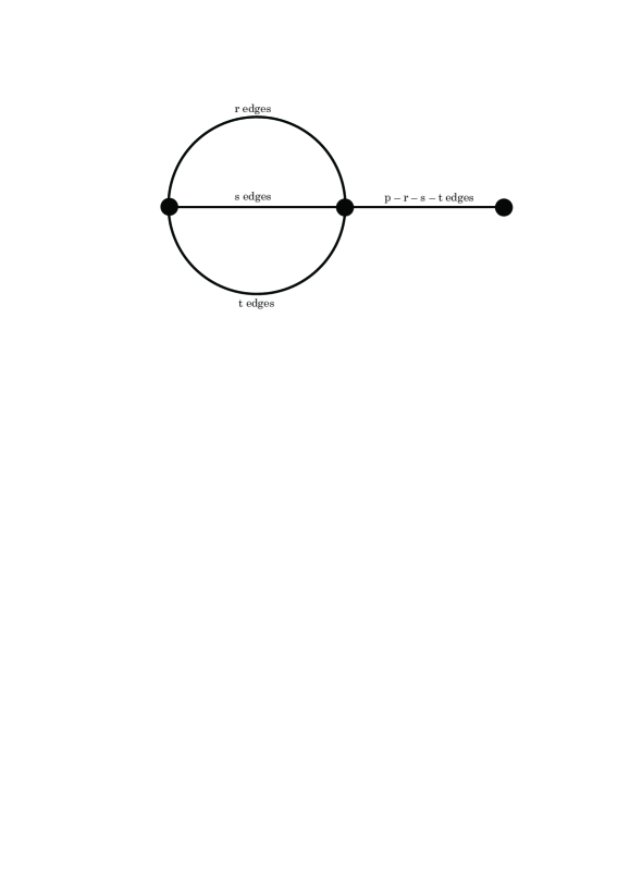
Figure 2: A graph for a regular $2^{p-2}$ fractional factorial design

It then follows that $D$ is the design matrix of $|E|$ factors with $2^{|V|-1}$ runs defined by (12). It is easy to see that $G$ has no $K_{4}$ minor. Hence, by virtue of Proposition 3.5, $I_{G}$ is generated by quadratic binomials. ∎

Remark 3.10.

Explicit description of binomials appearing in Theorem 3.9 is given in [18] and [10]. The set of generators of $I_{G}$ consisting of quadratic binomials for a regular $2^{p-1}$ fractional factorial design is studied in [2].

References

• [1] 4ti2 team. 4ti2 – A software package for algebraic, geometric and combinatorial problems on linear spaces. Available at www.4ti2.de.
• [2] S. Aoki (2013). Minimal Markov basis for tests of main effect models for $2^{p-1}$ fractional factorial designs of resolution $p$, preprint. arXiv:1302.2408.
• [3] S. Aoki, H. Hara and A. Takemura (2012). Markov bases in algebraic statistics. Springer Series in Statistics.
• [4] S. Aoki and A. Takemura (2009). Markov basis for design of experiments with three-level factors. in Algebraic and Geometric Methods in Statistics (dedicated to Professor Giovanni Pistone on the occasion of his sixty-fifth birthday), edited by P. Gibilisco, E. Riccomagno, M. P. Rogantin and H. P. Wynn, Cambridge University Press, 225–238.
• [5] S. Aoki and A. Takemura (2010). Markov chain Monte Carlo tests for designed experiments. Journal of Statistical Planning and Inference, 140, 817–830.
• [6] L. W. Condra (1993). Reliability Improvement with Design of Experiments. Marcel Dekker, New York, NY., 1993.
• [7] P. Diaconis and B. Sturmfels (1998). Algebraic algorithms for sampling from conditional distributions. Annals of Statistics, 26, 363–397.
• [8] R. Diestel (2010). Graph theory (4th edition), Graduate Texts in Mathematics 173, Springer-Verlag, Heidelberg.
• [9] A. Dobra (2003). Markov bases for decomposable graphical models. Bernoulli, 9, 1093–1108.
• [10] A. Engström (2011). Cut ideals of $K_{4}$-minor free graphs are generated by quadrics, Michigan Math. J. 60, no. 3, 705–714.
• [11] R. Fontana, G. Pistone and M. P. Rogantin (2000). Classification of two-level factorial fractions. Journal of Statistical Planning and Inference, 87, 149–172.
• [12] F. Galetto, G. Pistone and M. P. Rogantin (2003). Confounding revisited with commutative computational algebra. Journal of Statistical Planning and Inference, 117, 345–363.
• [13] D. K. Garnick, Y. H. H. Kwong and F, Lazebnik (1993). Extremal graphs without three-cycles or four-cycles, Journal of Graph Theory, 17, 633–645.
• [14] M. Hamada and J. A. Nelder (1997). Generalized linear models for quality-improvement experiments. Journal of Quality Technology, 29:292–304.
• [15] W. K. Hastings (1970). Monte Carlo sampling methods using Markov chains and their applications. Biometrika, 57, 97–109.
• [16] D. Král’, S. Norine and O. Pangrác (2010). Markov bases of binary graph models of $K_{4}$-minor free graphs, Journal of Combinatorial Theory, Series A, 117, 759–765.
• [17] P. McCullagh and J. A. Nelder (1989). Generalized linear models. 2nd ed. Chapman & Hall, London.
• [18] U. Nagel and S. Petrović (2009). Properties of cut ideals associated to ring graphs, J. Commutative Algebra, 1, no. 3, 547–565.
• [19] G. Pistone, E. Riccomagno and H. P. Wynn (2001). Algebraic Statistics: Computational Commutative Algebra in Statistics. Chapman & Hall, London.
• [20] G. Pistone and H. P. Wynn (1996). Generalised confounding with Gröbner bases. Biometrika, 83, 653–666.
• [21] B. Sturmfels and S. Sullivant (2008). Toric geometry of cuts and splits. Michigan Math. J., 57, 689–709.
• [22] C. F. Jeff Wu and M. Hamada (2000). Experiments: Planning, analysis, and parameter design optimization. Wiley Series in Probability and Statistics: Texts and References Section. John Wiley & Sons Inc., New York. A Wiley-Interscience Publication.