Ligand field parameters and the ground state of Fe(II) phthalocyanine

Abstract

A judicious analysis of previously published experimental data leads one to conclude that the ground state of iron(II) phthalocyanine is an orbitally degenerate spin triplet $a_{1g}^{2}e_{g}^{\uparrow\downarrow\uparrow}b_{2g}^{\uparrow}$ (${}^{3}E_{g}$). The ligand field parameters, in relation to Racah’s $C$, are approximately as follows: $B_{20}/C=0.84$, $B_{40}/C=0.0074$. The uniqueness of this result is demonstrated by means of a special diagram in the $B_{20}/C-B_{40}/C$ plane (under additional conditions that $B_{44}/B_{40}=35/3$ and $B/C=0.227$). The system is in a strong-ligand-field regime, which enables the use of single-determinant techniques corrected for correlations within the $3d$ shell of Fe.

I Introduction

Over several decades the interest in iron (II) phthalocyanine (FePc) has been motivated by various applications as well as by its proximity to iron proteins. In more recent times FePc has become popular as a model system for core-level spectroscopy (XAS, XMCD) studies.Miedema ; Stepanow ; Barto10 Certain progress has been made in creating artificial ordered structures of FePc.Abel ; Gredig Perhaps the most significant finding of the recent decade was the discovery of an unquenched orbital moment of iron in FePc by means of in-field Mössbauer spectroscopyFiloti and XMCD.Barto10

This has in turn brought about a surge of computational activity on FePc. Along with various density-functional calculations,ReynoldsFiggis ; LiaoScheiner ; MaromKronik ; KHO ; Brena ; Nakamura ; Wang ; Sumimoto ; Bialek it is worth to mention multiplet structure calculationsThole ; Miedema ; Stepanow based on a phenomenological model. The main ingredients of the latter approach are the Coulomb repulsion, allowed for by way of the Slater-Condon parameters, and the crystal (ligand) field (CF) on Fe²⁺. The multiplet calculationsThole ; Miedema ; Stepanow were mainly aimed at simulating x-ray absorption spectra; however, they produced an interesting by-product. This is a map of ground states of Fe²⁺ in CF parameter space (Fig. 2 of Ref. Miedema, ). An early version of such a diagram for the point group $D_{4h}$ was produced by König and Schnakig,KoenigS but the idea itself goes back to the classical work of Tanabe and Sugano,TS who dealt with the cubic symmetry. Unfortunately, in the case of $D_{4h}$ one cannot plot but 2-dimensional sections of the 3-dimensional space of CF parameters, the choice of these sections in Refs. KoenigS, and Miedema, being rather suboptimal. Besides, the diagrams in Refs. KoenigS, and Miedema, have the disadvantage that CF parameters in energy units are plotted on the axes, and so the diagrams depend on the Slater-Condon (or Racah) parameters employed. As against that, the original work of Tanabe and SuganoTS presented the result in terms of a dimensionless ratio of the CF parameter to Racah’s $B$, which led to the celebrated series of universal diagrams. Still, Miedema’s diagrams are of interest. They have an enigmatic cornered shape, the domain boundaries are piecewise-linear, with repeatedly encountered, characteristic slopes. These features of the diagrams have so far remained unexplained.

As regards agreement with experiment, the calculations leave much to be desired. Density-functional calculations make inconclusive predictions of the ground state. Thus, Reynolds and FiggisReynoldsFiggis could not decide between ${}^{3}E_{g}$ and ${}^{3}B_{2g}$ because the two lie too close in energy. Marom and KronikMaromKronik found either ${}^{3}B_{2g}$ ($e_{g}^{4}a_{1g}^{1}b_{2g}^{1}$) or ${}^{3}A_{2g}$ ($a_{1g}^{2}b_{2g}^{2}e_{g}^{\uparrow\uparrow}$), depending on computational details. remark1 More recently, Nakamura et al.Nakamura found ${}^{3}A_{2g}$ in an isolated FePc molecule, but ${}^{3}E_{g}$ in a columnar stack of such molecules. Establishing the symmetry of the ground state does not settle the dispute: within the correct ${}^{3}E_{g}$ one should further distinguish between the configurations $b_{2g}^{2}e_{g}^{3}a_{1g}^{1}$, as conjectured by Dale et al.,Dale and $a_{1g}^{2}e_{g}^{3}b_{2g}^{1}$, found in the multiplet calculations.Miedema ; Stepanow The two ground-state configurations lead to distinct types of magnetic behavior.

This work aims at determining the CF parameters of Fe(II) phthalocyanine. As we will show below, the known experimental facts on that compound (obtained by magnetic and spectroscopic measurements) in connection with our CF analysis leave no choice: there is only one domain in the field of CF parameters yielding a ground state that does not contradict established knowledge. In such a way our calculations resolve the confusing puzzle about the ground state of FePc that existed for many years. As a byproduct the peculiar shape of Miedema’s diagrams is explained.

In the following, we consider the $3d^{6}$ configuration in a CF of symmetry $D_{4h}$ and allow for Coulomb repulsion between the $3d$ electrons. The CF is a priori assumed neither strong nor weak as compared with the Coulomb interaction. Hybridization of the Fe $3d$ orbitals to neighboring ligands is thought to be included into the relevant CF parameters. In that sense it is better to call our theory ligand field theory instead. But the ligand $p$ orbitals are not treated in an explicit way and we keep the term CF theory for simplicity. The spin-orbit coupling is neglected at first (since it is much weaker than either the CF or the Coulomb repulsion) but taken into account in a later discussion of magnetic properties.

This paper is organized as follows. In the next section we briefly review the experimental facts that bear on our knowledge of the ground state of FePc and reiterate the current status of this knowledge. Further, in Section III, a diagram of ground states of FePc is constructed from numerical calculations. Our diagram is similar to that of Ref. Miedema, , the main two differences being that (i) dimensionless coordinates of the Tanabe-Sugano type are used and (ii) the section of the 3-dimensional space of CF parameters is chosen on the principle that the coordination polyhedron is a plane square. In Section IV, the same diagram is reproduced analytically, which includes explicit expressions for all domain boundaries. The subsequent discussion in Section V hinges upon the good agreement of the exact (numerical) and approximate (analytical) diagrams. The piecewise-linear shape of the domain boundaries finds a natural explanation in the linearity of the underlying equations. A conclusion is made that FePc is in a strong CF mode and approximate values of the CF parameters are given (or rather, ratios of CF parameters to Racah’s $C$). The ground-state configuration turns out to be $a_{1g}^{2}e_{g}^{3}b_{2g}^{1}$ (${}^{3}E_{g}$), as in Refs. Miedema, ; Stepanow, . Section VI recapitulates the conclusions.

II Experimental facts and their implications

II.1 Magnetic susceptibility

As early sources of our knowledge of the ground state of FePc one usually cites magnetic susceptibility studies of $\beta$-FePc powderDale and single crystals.Barraclough The experimental data of both papers are in reasonable agreement with each other. At temperatures between 100 and 300 K the susceptibility follows the Curie-Weiss law with $\mu_{\rm eff}\approx 3.8\,\mu_{\rm B}$ (for powder). This is between the spin-only values of $\mu_{\rm eff}$ for $S=1$ and $S=2$ ($2\sqrt{2}\,\mu_{\rm B}\approx 2.8\,\mu_{\rm B}$ and $2\sqrt{6}\,\mu_{\rm B}\approx 4.9\,\mu_{\rm B}$, respectively). Below about 20 K the susceptibility of $\beta$-FePc becomes temperature-independent.

These facts found an explanation in a simple model with $S=1$ and effective $g$-factors employed in both works.Dale ; Barraclough The spectrum of the model consists of a singlet ground state with $M_{S}=0$ and an excited doublet with $M_{S}=\pm 1$ situated at $\sim 70$ cm^-1. It is unclear why Dale et al.Dale thought to justify this model by proposing $b_{2g}^{2}e_{g}^{3}a_{1g}^{1}$ (${}^{3}E_{g}$) as the ground configuration (and calling it an orbital singlet). Their work contains no experimental evidence of ${}^{3}E_{g}$ being the ground state of FePc. Barraclough et al.Barraclough noticed the discrepancy between the orbitally degenerate ${}^{3}E_{g}$ and Dale’s assertion that the ground state should be an orbital singlet, and postulated ${}^{3}B_{2g}$ instead. As pointed out in Ref. StillmanTh, , this was no proof, ${}^{3}A_{2g}$ could have done equally well.

The model used in Refs. Dale, and Barraclough, is not without its difficulties. So, it cannot explain the presence of an excited state (or states) at $\sim 300$ cm^-1, as pointed out in Ref. Dale, . The existence of such an excited state follows from the fact that the susceptibility deviates from the Curie-Weiss law above room temperature, as observed by Lever.Lever (A slight downward curvature is also visible in $\chi^{-1}$ vs $T$ data obtained more recently on $\alpha$-FePc.Filoti ) This can be viewed as an argument in favor of ${}^{3}E_{g}$ rather than an orbital singlet. The six-fold degenerate ${}^{3}E_{g}$ would be split by the spin-orbit interaction into 4 singlets and a doublet, the overall splitting being $\sim\zeta\sim 400$ cm^-1. The observed susceptibility behavior would find a plausible explanation if one of the singlets was the ground state, the doublet (or a quasi-doublet) was situated at $\sim 70$ cm^-1, and a further state (or states) at $\sim 300$ cm^-1.

Another difficulty of Dale’s triplet model consists in the values of the $g$-factors, which differ significantly from 2. Thus, Dale et al.Dale obtain $g_{\perp}=2.86$ (and $g_{||}=1.93$). That is, nearly one Bohr magneton has to come from an orbital moment. Such a large orbital contribution is explained more naturally by the presence of an unquenched orbital moment (i.e., by orbital degeneracy of the ground state) rather than by mixing in of excited states. We note that Barraclough et al.,Barraclough who assert most emphatically the equivalence of their approach to that of Ref. Dale, , obtained an isotropic $g$-factor, $g_{\perp}=g_{||}=2.64$. Generally speaking, Barraclough’s $g$-factors should be more trustworthy, since they were deduced from data measured on a single crystal.Barraclough The difficulty, however, is that, according to Eq. (4) of Ref. Dale, , the zero-field splitting must vanish for $g_{\perp}=g_{||}$. At the same time, it is emphasized that this splitting, $\sim 70$ cm^-1, is very large.Barraclough

In any case, it should be regarded as firmly established that the susceptibility is a maximum in the plane of the FePc molecule.Barraclough This conclusion has been recently confirmed in an independent experiment.Barto10 As regards the ground states conjectured to explain the susceptibility data, they cannot be viewed as deduced from experiment.

II.2 Other techniques

An x-ray diffraction experiment of Coppens et al.Coppens found the occupation numbers of the Fe 3d orbitals in FePc: $b_{2g}^{1.65}e_{g}^{2.13}a_{1g}^{0.88}b_{1g}^{0.75}$. On account of covalency, these numbers sum up to 5.41 rather than 6. Restoring the normalization to 6, one has $b_{2g}^{1.83}e_{g}^{2.36}a_{1g}^{0.98}b_{1g}^{0.83}$. Coppens et al. regarded their result as a direct confirmation of Dale’s conjecture, $b_{2g}^{2}e_{g}^{3}a_{1g}^{1}$ (${}^{3}E_{g}$). Yet, the analysis in Ref. Coppens, was limited to spin-triplet states. An unprejudiced look at the quintet states, in particular at $b_{2g}^{2}e_{g}^{\uparrow\uparrow}a_{1g}^{\uparrow}b_{1g}^{\uparrow}$ (${}^{5}B_{2g}$), suggests a higher degree of agreement with Coppens’ results. However, ${}^{5}B_{2g}$ can be ruled out because it would have resulted in too high a magnetic moment, $\mu_{\rm eff}=4.9\,\mu_{\rm B}$.

Turning now to the optical absorption experiments of Stillman and Thomson,StillmanTh we note that they were carried out on FePc solution in dichlorobenzene. This system is chemically distinct from either the free FePc molecule or $\alpha$ or $\beta$ FePc. Therefore, without casting doubt upon Stillman and Thomson’s assertion of a ${}^{3}A_{2g}$ ground state, we state merely that their result is not relevant to the system under consideration herein.

A Mössbauer spectroscopy study of Filoti et al.Filoti found in $\alpha$-FePc a very large (66 T) hyperfine field on ⁵⁷Fe. Unlike the usual Fermi’s contact field, the hyperfine field in $\alpha$-FePc has a positive sign (meaning ${\bm{H}}_{\rm hf}\uparrow\uparrow{\bm{\mu}}_{\rm Fe}$) and can only originate from a large unquenched orbital moment. The latter was estimated to be about 1,Filoti but no definite information about its orientation could be obtained.

A more recent XMCD experiment of Bartolomé et al.Barto10 found in FePc an orbital moment of $0.53\,\mu_{\rm B}$ lying in the plane of the molecule. In the same workBarto10 it was demonstrated by direct measurements that the plane of the molecule contains the easy magnetization direction, in agreement with the early finding of Barraclough et al.Barraclough

To summarize the section, there is no experimental evidence of the ground state of FePc being either ${}^{3}B_{2g}$ or ${}^{3}A_{2g}$. Nor do Coppens’ dataCoppens provide sufficient confirmation for Dale’s conjecture of $b_{2g}^{2}e_{g}^{\uparrow\downarrow\uparrow}a_{1g}^{\uparrow}$ (${}^{3}E_{g}$). All one can say at this point is that it should be a ${}^{3}E_{g}$ state endowed with magnetic anisotropy of an easy-plane kind.

III Numerical calculations

III.1 Crystal field Hamiltonian

The CF Hamiltonian operating on a single $3d$ electron in a tetragonal ($D_{4h}$) environment is written as follows:

$${\cal H}_{\rm CF}=B_{20}O_{2}^{0}+B_{40}O_{4}^{0}+B_{44}O_{4}^{4}$$ (1)

Here $O_{n}^{m}$ are Stevens’ operator equivalentsStevens in the $\ell$-representation ($\ell=2$): $O_{2}^{0}=3\ell_{z}^{2}-6$, $O_{4}^{0}=35\ell_{z}^{4}-155\ell_{z}^{2}+72$, $O_{4}^{4}=\frac{1}{2}(\ell_{+}^{4}+\ell_{-}^{4})$; $B_{nm}$ are CF parameters. In older literature one sometimes comes across Ballhausen’s CF parameters.Ballhausen These are related to the $B_{nm}$’s in a simple way:

$$Dq=\textstyle\frac{12}{5}B_{44},~{}~{}~{}Ds=3B_{20},~{}~{}~{}Dt=\textstyle\frac{12}{5}B_{44}-12B_{40}$$ (2)

It is well known that the five real $d$ orbitals belong to distinct irreducible representations of the point group $D_{4h}$. Therefore, in the basis of those orbitals the CF Hamiltonian (1) takes a diagonal form, the eigenvalues beingBallhausen

$$\begin{array}[]{lcccl}E(d_{xy})&=&E(b_{2g})&=&6B_{20}+12B_{40}-12B_{44}\\ E(d_{xz,yz})&=&E(e_{g})&=&-3B_{20}-48B_{40}\\ E(d_{z^{2}})&=&E(a_{1g})&=&-6B_{20}+72B_{40}\\ E(d_{x^{2}-y^{2}})&=&E(b_{1g})&=&6B_{20}+12B_{40}+12B_{44}\end{array}$$ (3)

Note that Ballhausen’s original equations (5-14) and (5-15) need to be augmented with the cubic terms, $+6Dq$ and $-4Dq$, respectively, before being converted to the Stevens notation by means of Eqs. (2).

So far no restrictions have been imposed on the CF, except that it should be compatible with the point group $D_{4h}$. Yet, much more is known about the structure of the FePc molecule than just the symmetry of the Fe site. Thus, the nearest environment of the iron atom consists of four nitrogen atoms making a plane square, the Fe-N bonds being aligned with either the $x$ or the $y$ axis. This fact enables us to reduce the number of independent CF parameters by one. A rather general CF model known as the superposition model (see Ref. NewmanNg, for a comprehensive review), relates pairs of CF parameters $B_{nm}$ with equal $n$ on the basis of shape of the coordination polyhedron. Omitting the rather straightforward calculations, we state the result: for a plane square the superposition model demands that

$$B_{44}=\textstyle\frac{35}{3}B_{40}$$ (4)

III.2 Hamiltonian matrix

Our calculations dealt with a Hamiltonian consisting of the CF (1) and the Coulomb repulsion and operating on the $3d^{6}$ configuration. The basis states were taken in the form of simple products of one-electron $d$ orbitals,

$$\prod_{i=1}^{6}|m_{i}\sigma_{i}\rangle$$ (5)

with $m_{i}=0,\pm 1,\pm 2$, and $\sigma_{i}=\pm 1/2$. There are ${10\choose 6}=210$ such states in total.

Nonzero matrix elements of ${\cal H}_{\rm CF}$ (1) are of two kinds. First of all, there are diagonal matrix elements, given by

$$B_{20}\sum_{i=1}^{6}\left(3m_{i}^{2}-6\right)+B_{40}\sum_{i=1}^{6}\left(35m_{i}^{4}-155m_{i}^{2}+72\right)$$ (6)

Secondly, there are nonzero matrix elements between the states (5) that differ in one pair of quantum numbers $m_{i}$, $m_{i}$ being $-2$ in one of the states and $+2$ in the other one. All such matrix elements equal $12B_{44}$.

The matrix elements of the Coulomb repulsion have been treated extensively in the literature. Here we follow Griffith’s fundamental treatise.Griffith Again, there are two distinct kinds of nonzero matrix elements. The diagonal ones are given by

$$\sum_{k=0,2,4}F^{k}\sum_{i>j}\left[c_{m_{i}m_{i}}^{k}c_{m_{j}m_{j}}^{k}-\delta_{\sigma_{i}\sigma_{j}}\left(c_{m_{i}m_{j}}^{k}\right)^{2}\right]$$ (7)

where $F^{k}$ are the Slater-Condon parameters ($k=0,2,4$) and

$$c_{mm^{\prime}}^{k}=\sqrt{\frac{4\pi}{2k+1}}\int Y_{2m}^{*}Y_{2m^{\prime}}Y_{k,m-m^{\prime}}d\Omega$$ (8)

The integral in Eq. (8) is known as the Gaunt coefficient. Numerical values of $c_{mm^{\prime}}^{k}$ were taken from Table 4.4 of Griffith’s book.Griffith The inner sum in Eq. (7) is taken over all 15 pairs of filled $d$ orbitals. The first term in brackets describes the so-called Coulomb contribution, while the second one, relevant to pairs of orbitals with parallel spins only, is the exchange contribution.

The Coulomb repulsion also has off-diagonal matrix elements. These are nonzero only between the states with equal $M_{L}$ and $M_{S}$ that differ in two occupied $d$ orbitals, say, $|m_{i1}\sigma_{i1}\rangle$ and $|m_{j1}\sigma_{j1}\rangle$ in State #1, as against $|m_{i2}\sigma_{i2}\rangle$ and $|m_{j2}\sigma_{j2}\rangle$ in State #2. It must hold that $m_{i1}+m_{j1}=m_{i2}+m_{j2}$ and $\sigma_{i1}+\sigma_{j1}=\sigma_{i2}+\sigma_{j2}$. The matrix element between the states #1 and #2 is expressed as follows

$$\sum_{k=0,2,4}F^{k}\left[\delta_{\sigma_{i1}\sigma_{i2}}\delta_{\sigma_{j1}\sigma_{j2}}c_{m_{i1}m_{i2}}^{k}c_{m_{j2}m_{j1}}^{k}\right.$$

$$\left.-\delta_{\sigma_{j1}\sigma_{i2}}\delta_{\sigma_{i1}\sigma_{j2}}c_{m_{j1}m_{i2}}^{k}c_{m_{j2}m_{i1}}^{k}\right]$$ (9)

Thus, the matrix elements of the Hamiltonian are linear combinations of the CF parameters, $B_{20}$, $B_{40}$, and $B_{44}$, as well as the Slater-Condon parameters, $F^{0}$, $F^{2}$, and $F^{4}$. The latter are conveniently replaced by the Racah parameters,

$$F^{0}=A+\textstyle\frac{7}{5}C,~{}~{}~{}F^{2}=49B+7C,~{}~{}~{}F^{4}=\textstyle\frac{63}{5}C$$ (10)

The parameter $A$ is hereafter set to zero, because its only effect is to shift the energies of all the states of $d^{n}$ by the same amount, $An(n-1)/2$.

III.3 Degeneracy diagram

The calculation consisted in setting and numerically diagonalizing the Hamiltonian matrix for given sets of parameters $B_{20}$, $B_{40}$, $B_{44}$, $B$, $C$, and subsequently determining the degeneracy of the ground state. Five characteristic values of degeneracy were encountered:

$$\begin{array}[]{rcl}1:&~{}~{}~{}~{}^{1}A{}{}{}{}&S=0,~{}{\rm no~{}orbital~{}degeneracy}\\ 3:&{}^{3}A&S=1,~{}{\rm no~{}orbital~{}degeneracy}\\ 5:&{}^{5}A&S=2,~{}{\rm no~{}orbital~{}degeneracy}\\ 6:&{}^{3}E&S=1,~{}{\rm double~{}orbital~{}degeneracy}\\ 10:&{}^{5}E&S=2,~{}{\rm double~{}orbital~{}degeneracy}\end{array}$$

At this stage the ground states are labeled tentatively. So $A$ can be anything of the following: $A_{1g}$, $A_{2g}$, $B_{1g}$, or $B_{2g}$, which we are unable to distinguish. On the other hand, ${}^{3}E$=${}^{3}E_{g}$ and ${}^{5}E$=${}^{5}E_{g}$ as will be explained in Section IV.

The construction of the diagram (Figure 1) was organized as follows. All energies were expressed in the units of the Racah parameter $C$. The ratios $B_{20}/C$ and $B_{40}/C$ were treated as independent variables defined on a dense mesh. In the spirit of Tanabe and Sugano,TS the ratio $B/C$ was fixed to a value appropriate for Fe²⁺, $B/C=0.227$, as in Table 7.3 of Ref. AB, . The CF parameter $B_{44}$ was not regarded as an independent one. Rather, it was found from Eq. (4), as prescribed by the superposition model.NewmanNg As a result, the $B_{20}/C-B_{40}/C$ plane was partitioned into domains of five different kinds, according to the degeneracy found at each point. The diagram (Figure 1) has a cornered shape reminiscent of the diagrams in Refs. Miedema, and KoenigS, . The domain boundaries appear straight lines with characteristic slopes. Several sets of parallel lines are encountered. The central part of the diagram is an area of weak CF; in compliance with Hund’s first rule, the ground state here has $S=2$. The periphery of Figure 1 is a region of strong CF; here $S=0$ or 1.

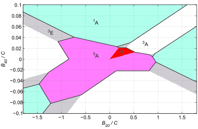
Figure 1: Partition of CF parameter space among differently degenerate ground states, as found from numerical calculations in the absence of spin-orbit interaction. The possible ground states are denoted according to their total spin and the absence (${}^{2S+1}A$) or presence (${}^{2S+1}E$) of orbital degeneracy. They will be further specified in Figure 3.

The numerical calculations have the advantage of producing an immediate graphical result. However, it is not easy to analyze the character of a ground state expressed in a 210-dimensional basis. Of special interest to us is ${}^{3}E_{g}$, which appears in six non-adjacent domains in Figure 1. So we would like to know if those ${}^{3}E_{g}$ are similar or distinct. Furthermore, we would like to find out the origin of the cornered shape of the diagram, why the boundaries are straight and the slopes repeated. Finally, we pose a question, how the diagram would change if $B/C$ and/or $B_{44}/B_{40}$ were different to the ones used so far. Answers to the above questions should be sought by means of analytical calculations.

IV Analytical treatment

IV.1 Weak crystal field: quintet states

In the weak-field approximation the CF is treated as a perturbation with respect to the intra-atomic Coulomb interaction, whose eigenstates are spectral terms with certain $L$ and $S$. Since the CF acts on spatial but not on spin variables, terms with different $S$ do not mix together (as long as the spin-orbit coupling is neglected). In the $d^{6}$ configuration there is a single quintet term, ${}^{5}D$, whose Coulomb energy isGriffith

$$E_{\rm Coulomb}=-35B+7C$$ (11)

The remaining task consists in diagonalizing the CF Hamiltonian (1) on the wave functions of ${}^{5}D$, since there are no other terms with $S=2$. To this end, it is convenient to interpret Eq. (1) in a slightly different way than it was done in Section III. Namely, $O_{n}^{m}$ are now regarded as Stevens’ operators in the $L$ representation ($L=2$): $O_{2}^{0}=3L_{z}^{2}-6$ etc. Since ${}^{5}D$ contains a single $d$ electron above a closed semi-shell, it is only this one electron that is exposed to the CF. Therefore, $L=\ell$ and the coefficients $B_{nm}$ in Eq. (1) are the same in both representations. So we can simply take over the one-electron CF energies (3). In doing so, we capitalize the irrep labels, to indicate that they now refer to many-electron states, and append the multiplicity 5. We also prefix $E_{\rm Coulomb}$ (11). The resulting energies of the quintet states are as follows:

$$\begin{array}[]{lll}E(^{5}B_{2g})&=-35B+7C+6B_{20}+12B_{40}-12B_{44}&~{}({\rm Q1})\\ E(^{5}E_{g})&=-35B+7C-3B_{20}-48B_{40}&~{}({\rm Q2})\\ E(^{5}A_{1g})&=-35B+7C-6B_{20}+72B_{40}&~{}({\rm Q3})\\ E(^{5}B_{1g})&=-35B+7C+6B_{20}+12B_{40}+12B_{44}&~{}({\rm Q4})\end{array}$$

IV.2 Strong crystal field: singlet states

In the strong-CF approximation the zeroth-order states are constructed from one-electron eigenstates of the CF Hamiltonian (1), then their energies are corrected for the Coulomb repulsion. A first question that arises is: which six one-electron $d$ states are filled in a CF of symmetry $D_{4h}$? To give a possibly general answer, it is convenient to express all relevant energies in the units of $B_{44}$. Thus, the one-electron CF energies (3) are divided by $B_{44}$. Then, equating pairs of the so modified expressions, one obtains 5 equations linear in $B_{20}/B_{44}$ and $B_{40}/B_{44}$. The corresponding lines in the parameter plane $B_{20}/B_{44}-B_{40}/B_{44}$ (Figure 2) are loci of points where the sequence of CF levels changes. For example, the levels $a_{1g}$ and $b_{1g}$ cross over on a line decribed by

$$-B_{20}/B_{44}+5B_{40}/B_{44}=1$$ (12)

as readily obtained by equating the last two Eqs. (3). Equation (12) describes the upper one of the two parallel lines in Figure 2; the lower line arises from the condition $E(a_{1g})=E(b_{2g})$. Likewise, the equation $E(e_{g})=E(b_{1g,2g})$ generates a pair of parallel lines with a negative slope. A single line passing through the origin is produced by the relation $E(a_{1g})=E(e_{g})$. Finally, the equation $E(b_{1g})=E(b_{2g})$ leads to no line; this is why there are 5 solid lines in Figure 2, rather than 6 as expected combinatorially. The CF levels $b_{1g}$ and $b_{2g}$ do not swap at any inner point of Figure 2, but do so at infinity, where $B_{44}$ changes sign. Therefore, $b_{2}$ (a short for $b_{2g}$) stands always to the left of $b_{1}$ ($b_{1g}$) in the level sequences indicated within each one of the 12 domains. The sequence labels, read from left to right, name the CF levels in order of ascending energy if $B_{44}>0$, and in order of descending energy if $B_{44}<0$.

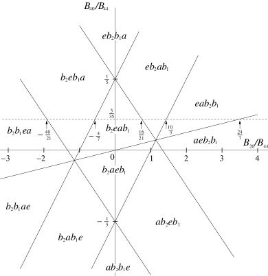
Figure 2: Partition of the $B_{20}/B_{44}-B_{40}/B_{44}$ plane among all possible permutations of the four one-electron CF levels.

Up to this point no restrictions have been placed on the CF, apart from those imposed by the $D_{4h}$ symmetry. Now we do restrict the CF by demanding that it must additionally comply with the superposition model, Eq. (4). This implies that the system is now bound to the horizontal dashed line in Figure 2. The dashed line cuts through six domains. The corresponding intervals on the abscissa axis are numbered 1 to 6 in order of ascending $B_{20}/B_{44}$, with $B_{44}>0$. Thus, the interval #1 stands for $B_{20}/B_{44}<-\frac{40}{21}$, #2 means that $-\frac{40}{21}<B_{20}/B_{44}<-\frac{4}{7}$ etc. The same intervals, but with $B_{44}<0$, will be referred to by overscore numbers $\overline{1}$ to $\overline{6}$.

Now, examining the CF level sequences in the above 12 intervals, one encounters only 3 situations where there is a CF gap between the highest occupied and the lowest unoccupied orbitals. The corresponding ground-state electronic configurations are as follows:

$$\begin{array}[]{ll}b_{2g}^{2}e_{g}^{4}&{\rm~{}intervals}~{}\#2,\,\#3,\,\#4\\ a_{1g}^{2}e_{g}^{4}&{\rm~{}intervals}~{}\#5,\,\#6,\,\#\overline{1}\\ a_{1g}^{2}b_{1g}^{2}b_{2g}^{2}&{\rm~{}intervals}~{}\#\overline{4},\,\#\overline{5}\end{array}$$ (13)

Within the above intervals of $B_{20}/B_{44}$ the ground state is a singlet, provided that the CF is sufficiently strong. In all other cases the Fermi level is caught at the partially occupied quadruply degenerate $e_{g}$ level and there is a possibility of both a singlet and a (spin) triplet ground state with the same energy. A subsequent allowance for intra-atomic (Hund’s) exchange makes the triplet states energetically more favorable than the singlet ones. Therefore, singlets are no viable candidates for ground state in all intervals where triplets with the same CF energy are possible. In such intervals only the triplets will be considered (in the next subsection).

Conversely, in the three cases where there are viable singlet states (13), competing triplet states will be taken into consideration as well, constructed from excited CF configurations. Such triplets still have a chance of becoming ground state on account of Hund’s exchange in situations where the CF is not strong enough, near interval boundaries, etc.

Let us now turn to our direct task — computing the energies of the singlet states (13). The CF energies are computed most readily, by summing up the energies of the six occupied one-electron states as given by Eqs. (3). First-order correlation corrections are then computed following Slater’s prescription:Slater for each pair of occupied $d$ states a so-called Coulomb integral $J(d_{1},d_{2})$ is added; a further exchange contribution $K(d_{1},d_{2})$ is deducted for pairs with equal spins. $J$’s and $K$’s between the real $d$ orbitals were expressed in terms of the Racah parameters by Griffith, see Table A26 of his book.Griffith The resulting singlet energies are as follows:

$$\begin{array}[]{lcrl}E(b_{2g}^{2}e_{g}^{4})&=&-168B_{40}-24B_{44}-30B+15C&~{}~{}({\rm S1})\\ E(a_{1g}^{2}e_{g}^{4})&=&-24B_{20}-48B_{40}+10B+15C&~{}~{}({\rm S2})\\ E(a_{1g}^{2}b_{1g}^{2}b_{2g}^{2})&=&12B_{20}+192B_{40}-20B+15C&~{}~{}({\rm S3})\end{array}$$

We note that for low-lying single-product states, such as those considered in this work, the factor of $C$ depends solely on $S$ and is given by

$$({\rm factor~{}of~{}}C)=(S_{\max}+1)^{2}-(S+1)^{2}$$ (14)

where $S_{\max}=n/2$ is the hypothetical maximum spin of $n$ electrons in the absence of the Pauli principle. For fewer than six $d$ electrons, states with $S=S_{\max}$ are allowed and their energies have no contribution in $C$. For $d^{6}$, $S_{\max}=3$ and the factors of $C$ equal 15, 12, and 7 for $S=0$, 1, and 2, respectively. Equation (14) is a consequence of the great simplicity acquired by the Coulomb and exchange integrals when $A$ and $B$ are set to zero:

$$J(d_{i},d_{j})=K(d_{i},d_{j})=(1+2\delta_{ij})C,$$

cf. Table A26 of Ref. Griffith, . No simple relations are known for the factors of $B$, which have to be calculated in each case separately.

IV.3 Strong crystal field: triplet states

Construction and finding the energies of the (spin) triplet states are carried out in a similar fashion. One peculiarity is the large number of triplets (9 in total), which have to be constructed for all 12 intervals of $B_{20}/B_{44}$. Where no triplet state is permitted by the ground CF configuration, the first excited configuration will be considered instead.

We proceed from the interval #1, $B_{20}/B_{44}<-\frac{40}{21}$, $B_{44}>0$. Here (as well as in the interval #$\overline{6}$, $B_{20}/B_{44}>\frac{24}{7}$, $B_{44}<0$) the ground CF configuration is $b_{1g}^{2}b_{2g}^{2}e_{g}^{2}$, which allows one triplet state, $d_{x^{2}-y^{2}}^{2}d_{xy}^{2}d_{xz}^{\uparrow}d_{yz}^{\uparrow}$, as well as three singlet ones. According to the first Hund’s rule, it will be the triplet that will become ground state upon allowance for the Coulomb interaction. (It was for this reason that the singlets were left out in the previous subsection.) The symmetry of the triplet state is ${}^{3}A_{2g}$, as determined by the antisymmetrized product of $d_{xz}$ and $d_{yz}$. The energy is computed following the same prescription as in the previous subsection and equals

$$E(b_{1g}^{2}b_{2g}^{2}e_{g}^{\uparrow\uparrow})=18B_{20}-48B_{40}-9B+12C~{}~{}~{}~{}~{}~{}({\rm T1})$$

Let us move to the interval #2, $-\frac{40}{21}<B_{20}/B_{44}<-\frac{4}{7}$, $B_{44}>0$. The ground CF configuration, $b_{2g}^{2}e_{g}^{4}$, consists of fully occupied orbitals and is necessarily a singlet. To construct a spin triplet state, one spin-down electron is promoted, with a simultaneous reversal of spin, from the $e_{g}$ orbital to the first unoccupied CF level $b_{1g}$. The result is either $d_{xy}^{2}d_{xz}^{2}d_{yz}^{\uparrow}d_{x^{2}-y^{2}}^{\uparrow}$ or $d_{xy}^{2}d_{yz}^{2}d_{xz}^{\uparrow}d_{x^{2}-y^{2}}^{\uparrow}$. This is a doubly orbitally degenerate state ${}^{3}E_{g}$. Its energy is

$$E(b_{2g}^{2}e_{g}^{\uparrow\downarrow\uparrow}b_{1g}^{\uparrow})=9B_{20}-108B_{40}-12B_{44}-24B+12C~{}~{}~{}({\rm T2})$$

Proceeding as before, we find that the most favorable spin triplet state in the interval #3 is another ${}^{3}E_{g}$, whose energy is given by

$$E(b_{2g}^{2}e_{g}^{\uparrow\downarrow\uparrow}a_{1g}^{\uparrow})=-3B_{20}-48B_{40}-24B_{44}-28B+12C~{}~{}~{}({\rm T3})$$

The remaining six spin-triplet states include: a ${}^{3}B_{2g}$ in the intervals #4 and #5, with

$$E(e_{g}^{4}b_{2g}^{\uparrow}a_{1g}^{\uparrow})=-12B_{20}-108B_{40}-12B_{44}-22B+12C~{}~{}~{}({\rm T4})$$

a ${}^{3}E_{g}$ in the interval #6, with

$$E(a_{1g}^{2}e_{g}^{\uparrow\downarrow\uparrow}b_{2g}^{\uparrow})=-15B_{20}+12B_{40}-12B_{44}-14B+12C~{}~{}({\rm T5})$$

a ${}^{3}E_{g}$ in the interval #$\overline{1}$, with

$$E(a_{1g}^{2}e_{g}^{\uparrow\downarrow\uparrow}b_{1g}^{\uparrow})=-15B_{20}+12B_{40}+12B_{44}-14B+12C~{}~{}({\rm T6})$$

a ${}^{3}A_{2g}$ in the intervals #$\overline{2}$ and #$\overline{3}$, with

$$E(a_{1g}^{2}b_{1g}^{2}e_{g}^{\uparrow\uparrow})=-6B_{20}+72B_{40}+24B_{44}-29B+12C~{}~{}~{}({\rm T7})$$

a ${}^{3}E_{g}$ in the interval #$\overline{4}$, with

$$E(a_{1g}^{2}b_{1g}^{2}b_{2g}^{\uparrow}e_{g}^{\uparrow})=3B_{20}+132B_{40}+12B_{44}-29B+12C~{}~{}({\rm T8})$$

and a ${}^{3}E_{g}$ in the interval #$\overline{5}$, with

$$E(b_{1g}^{2}b_{2g}^{2}a_{1g}^{\uparrow}e_{g}^{\uparrow})=15B_{20}+72B_{40}-13B+12C~{}~{}~{}~{}({\rm T9})$$

Note that the factor of $C$ in Eqs. (T1–T9) is invariably 12, as follows from Eq. (14) with $S=1$ and $S_{\max}=3$.

IV.4 The $B_{20}/C-B_{40}/C$ diagram

The search for the ground state consists in a systematic comparison of energies of pairs of candidate states, as given by Eqs. (Q1-Q4, S1-S2, T1-T9). For example, equating (Q1) to (T1) results in

$$-12B_{20}+60B_{40}-12B_{44}=26B+5C$$ (15)

Eliminating $B_{44}$ by means of Eq. (4) and dividing the result by $C$, one arrives at an equation of a straight line in the plane of the parameters $B_{20}/C$ and $B_{40}/C$:

$$\frac{B_{40}}{C}=-0.15\frac{B_{20}}{C}-0.0625-0.325\frac{B}{C}$$ (16)

Left of this line there should be a domain where the ground state is the triplet $T_{1}$ (${}^{3}A_{2g}$ or $b_{1g}^{2}b_{2g}^{2}e_{g}^{\uparrow\uparrow}$), right of the line, towards the origin, lies the domain where the ground state is the quintet $Q_{1}$ (${}^{5}B_{2g}$). In the spirit of Tanabe-Sugano, the ratio $B/C$ is fixed, $B/C=0.227$, as in Table 7.3 of Ref. AB, .

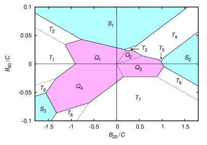
Figure 3: Partition of CF parameter space among possible ground states of FePc. The labels are mnemonic: so $S_{1}$ is a singlet whose energy is given by Eq. (S1). The borderlines are as described by Eq. (17) with the coefficients of Table I.

Proceeding as above, one obtains equations for all 33 borderlines appearing in the diagram, Figure 3. (It suffices to consider pairs of states belonging to the same, or perhaps, to adjacent intervals of $B_{20}/B_{44}$.) By analogy with Eq. (16), these expressions are presented as

$$\frac{B_{40}}{C}=a\frac{B_{20}}{C}+b+b^{\prime}\frac{B}{C}$$ (17)

The numerical factors $a$, $b$, and $b^{\prime}$ are listed in Table I. A line is referred to by naming the two domains it separates. Remarkably, one finds in the second column of Table I repeatedly six characteristic slopes,

$$0,-\textstyle\frac{9}{200},-\frac{3}{20},\frac{9}{80},\frac{3}{50},{\rm~{}and~{}}\frac{1}{40}.$$ (18)

These are obtained by means of Eq. (4) from the interval boundaries in Figure 2: so $B_{20}/B_{44}=24/7$ leads to $B_{20}/B_{40}=1/40$ etc. One exception that is not on the list (18) but is encountered twice in the second column of Table I is $-3/160$.

Table 1: Values of coefficients in Eq. (17).

label	$a~{}~{}~{}$	$b~{}~{}~{}$	$b^{\prime}~{}~{}~{}~{}~{}~{}$
$T_{1}Q_{1}$	$-3/20$	$-1/16$	$-13/40~{}~{}~{}$
$T_{2}Q_{1}$	$1/40$	$1/24$	$11/120~{}~{}~{}$
$T_{1}T_{2}$	$-9/200$	$0$	$-3/40~{}~{}~{}$
$~{}~{}~{}~{}S_{1}T_{2}$	$~{}~{}~{}~{}-9/200$	$~{}~{}~{}~{}~{}3/200$	$~{}~{}~{}~{}-3/100~{}~{}~{}$
$S_{1}Q_{1}$	$-3/160$	$1/40$	$1/64~{}~{}~{}$
$S_{1}T_{3}$	$1/40$	$1/40$	$-1/60~{}~{}~{}$
$S_{1}T_{4}$	$3/50$	$3/200$	$-1/25~{}~{}~{}$
$T_{3}Q_{1}$	$-9/200$	$1/40$	$7/200~{}~{}~{}$
$T_{3}Q_{2}$	$0$	$1/56$	$1/40~{}~{}~{}$
$T_{4}Q_{2}$	$-9/200$	$1/40$	$13/200~{}~{}~{}$
$T_{4}Q_{3}$	$-3/160$	$1/64$	$13/320~{}~{}~{}$
$T_{5}Q_{3}$	$-9/200$	$1/40$	$21/200~{}~{}~{}$
$S_{2}Q_{3}$	$-3/20$	$1/15$	$3/8~{}~{}~{}$
$S_{2}T_{5}$	$9/80$	$-3/80$	$-3/10~{}~{}~{}$
$S_{2}T_{4}$	$3/50$	$-3/200$	$-4/25~{}~{}~{}$
$Q_{1}Q_{2}$	$9/80$	$0$	$0~{}~{}~{}$
$Q_{2}Q_{3}$	$1/40$	$0$	$0~{}~{}~{}$
$T_{3}T_{4}$	$9/80$	$0$	$-3/40~{}~{}~{}$
$T_{4}T_{5}$	$1/40$	$0$	$-1/15~{}~{}~{}$
$T_{6}Q_{3}$	$9/80$	$-1/16$	$-21/80~{}~{}~{}$
$T_{7}Q_{3}$	$0$	$-1/56$	$-3/140~{}~{}~{}$
$T_{7}Q_{4}$	$3/50$	$-1/40$	$-3/100~{}~{}~{}$
$S_{2}T_{6}$	$-9/200$	$3/200$	$3/25~{}~{}~{}$
$T_{6}T_{7}$	$-9/200$	$0$	$3/40~{}~{}~{}$
$Q_{3}Q_{4}$	$-3/20$	$0$	$0~{}~{}~{}$
$T_{8}Q_{4}$	$1/40$	$-1/24$	$-1/20~{}~{}~{}$
$T_{7}T_{8}$	$9/80$	$0$	$0~{}~{}~{}$
$S_{3}Q_{4}$	$-3/20$	$-1/5$	$-3/8~{}~{}~{}$
$S_{3}T_{8}$	$9/80$	$3/80$	$9/80~{}~{}~{}$
$T_{9}Q_{4}$	$9/80$	$1/16$	$11/40~{}~{}~{}$
$S_{3}T_{9}$	$1/40$	$-1/40$	$7/120~{}~{}~{}$
$T_{1}Q_{4}$	$3/50$	$1/40$	$13/100~{}~{}~{}$
$T_{1}T_{9}$	$1/40$	$0$	$1/30~{}~{}~{}$

V Discussion

In the preceeding section we constructed a diagram of ground states of FePc in the absence of spin-orbit coupling, Figure 3. A total of 16 distinct ground states are present in the diagram: 3 singlets ($S_{1}-S_{3}$), 9 spin triplets ($T_{1}-T_{9}$), and 4 spin quintets ($Q_{1}-Q_{4}$). The respective energies are given by Eqs. (S1-S3, T1-T9, Q1-Q4). Explicit expressions were derived for the domain boundaries, Eq. (17) and Table I. The boundaries are segments of straight lines, which is a consequence of the linearity of Eqs. (S1-S3, T1-T9, Q1-Q4). This gives the diagram its peculiar cornered shape, with characteristic, repeated slopes. As clear from the structure of Eq. (17), the slopes do not depend on the ratio $B/C$. Taking a slightly different $B/C$ would shift the domain boundaries somewhat, but will not affect their slopes. As against that, the slopes will change if the ratio $B_{44}/B_{40}$ deviates from the value prescribed by the superposition model, Eq. (4). Moreover, such a deviation of $B_{44}/B_{40}$ from 35/3 may lead to a loss of parallelity of certain boundary lines. For example, from a simple analysis of the one-electron CF energies (3) one finds

$$\begin{array}[]{l}({\rm slope~{}of~{}}T_{1}Q_{1})=({\rm slope~{}of~{}}Q_{3}Q_{4})=(5-B_{44}/B_{40})^{-1}\\ ({\rm slope~{}of~{}}S_{3}Q_{4})=(2B_{44}/B_{40}-30)^{-1}\\ ({\rm slope~{}of~{}}S_{2}Q_{3})=-3/20\end{array}$$

Apparently the above lines are only parallel if the condition (4) is fulfilled. In reality the superposition model is an approximation and small deviations from Eq. (4) are to be expected. In the above example, the borderlines $T_{1}Q_{1}$ and $Q_{3}Q_{4}$ will remain parallel exactly, while the others only approximately. A more extensive analysis of this matter is beyond the scope of the present work.

On the whole, the diagram constructed analytically (Figure 3) is remarkably similar to that calculated numerically (Figure 1). We take it as a sign of validity of the strong-CF approximation used to compute the energies of the singlet and triplet states, Eqs. (S1-S3, T1-T9). (N.B. The quintet energies (Q1-Q4) are essentially exact, without relying on the weakness of the CF.) This demonstrates the applicability of techniques based on single-determinant wave functions, even though it is important to allow for correlations (nonzero $B$ and $C$).

Our next task is to locate the standpoint of FePc in the diagrams of Figures 1 and 3. In the subsequent discussion the domain boundaries are assumed to be positioned as in the more accurate Figure 1, whereas the ground states associated with the domains are as constructed analytically and indicated in Figure 3. The search can be limited to an acute angle adjacent to the abscissa axis, within the first quadrant of Figure 3:

$$0<B_{40}<0.45B_{20}$$ (19)

Indeed, the $d_{x^{2}-y^{2}}$ orbital of Fe overlaps most strongly with the ligand orbitals and therefore has a much higher energy than the other $3d$ orbitals, in particular, $d_{xy}$. By Eqs. (3), $E(d_{x^{2}-y^{2}})-E(d_{xy})=24B_{44}>0$, whence by Eq. (4), $B_{40}>0$. To prove the right-hand part of the double inequality (19), one should rewrite the CF Hamiltonian (1), taken in conjunction with Eq. (4), as a classical anisotropy energy,

$$E_{a}=B_{20}(3\cos^{2}\theta-1)~{}~{}~{}~{}~{}~{}~{}~{}~{}~{}~{}~{}~{}~{}~{}~{}~{}~{}~{}~{}~{}~{}~{}~{}~{}~{}$$

$$+B_{40}(35\cos^{4}\theta-30\cos^{2}\theta+3+\textstyle\frac{35}{3}\sin^{4}\theta\cos 4\phi)$$

and demand that $\theta=\pi/2$, $\phi=\pi/4$ be a local minimum. This is to account for the well established fact that the easy magnetization direction lies in the plane of the FePc molecule.Barraclough ; Barto10

A further experimental fact to take into consideration is that the ground state is a spin triplet ($S=1$) and that is is orbitally degenerate (${}^{3}E_{g}$).Filoti ; Barto10 Within the sector defined by the condition (19) there are only two domains where ${}^{3}E_{g}$ is the ground state — a quadrangle $T_{3}$ and a triangle $T_{5}$. We carried out an extensive numerical study of the magnetic susceptibility (with due allowance for the spin-orbit coupling) and found that $\chi_{||}(T)>\chi_{\perp}(T)$ everywhere within $T_{3}$, but $\chi_{||}(T)<\chi_{\perp}(T)$ inside $T_{5}$. (Here the subscript ”$||$” refers to the direction parallel to the 4-fold symmetry axis.) One has to conclude, therefore, that the standpoint of FePc in Figure 3 lies inside the triangle $T_{5}$. The corresponding ground-state configuration is $a_{1g}^{2}e_{g}^{\uparrow\downarrow\uparrow}b_{2g}^{\uparrow}$, cf. Eq. (T5). It is distinct from the configuration $T_{3}$, or $b_{2g}^{2}e_{g}^{\uparrow\downarrow\uparrow}a_{1g}^{\uparrow}$, postulated by Dale et al.Dale and adopted by Filoti et al.Filoti On a simple model the latter authors have demonstrated that $T_{3}$ has necessarily an easy-axis anisotropy, which agrees with our analysis. The experiment,Barraclough ; Barto10 however, insists on an easy-plane anisotropy and so $T_{3}$ has to be definitively abandoned. After all, Dale’s choice of $T_{3}$ was a mere conjecture, without a sufficient experimental foundation. It should also be noted that Miedema et al.Miedema ; Stepanow proceeded from the correct ground-state configuration $T_{5}$, even though they did not explain their choice.

Figure 4: Temperature dependence of reciprocal susceptibility. Closed circles are experimental data,Barraclough solid line is 1.22 times the calculated $\chi^{-1}$.

The difference between the two ${}^{3}E_{g}$ configurations is easy to understand. In both cases there is one $e_{g}$ hole; the two real $e_{g}$ orbitals ($d_{xz}$ and $d_{yz}$) can be combined to give states with $\ell_{z}=\pm 1$. An extra singly occupied orbital in $T_{3}$ is $a_{1g}$ ($d_{z^{2}}$), with $\ell_{z}=0$. Therefore, the z-component of the total orbital moment is $L_{z}=\pm 1$ and the spin-orbit coupling leads to an easy-axis anisotropy in $T_{3}$. In $T_{5}$ it is the $d_{xy}$ orbital ($b_{2g}$) that is singly occupied and the situation is quite different. Now three orbitals, $d_{xy}$, $d_{xz}$, and $d_{yz}$, are accessible to the holes. If the $e_{g}$ and $b_{2g}$ levels were perfectly degenerate, there would be no anisotropy at all. The fact that the degeneracy is lifted results in a weak easy-plane anisotropy, such as the one observed.

We undertook an attempt to refine the position of the system inside the triangle $T_{5}$ on the basis of the available susceptibility data.Barraclough We find that the most likely standpoint is near the left corner of the triangle, at $B_{20}/C=0.84$, $B_{40}/C=0.0074$. Powder susceptibility was calculated as $\frac{1}{3}\chi_{||}+\frac{2}{3}\chi_{\perp}$, with $B=917\,{\rm cm}^{-1}$ and $C=4040\,{\rm cm}^{-1}$ (as in Table 7.3 of Ref. AB, ). The spin-orbit coupling constant $\zeta$ was set to $400\,{\rm cm}^{-1}$. The so computed susceptibility proved higher than the experimental one and had to be reduced by a factor of 0.8, to make both curves match. (Accordingly, in Fig. 4 the experimental reciprocal susceptibilityBarraclough is compared with the calculated $\chi^{-1}$ times 1.22.) The reduction factor 0.8 can be attributed to covalency, neglected in our model.

Apart from the rescaling, the calculated $\chi^{-1}(T)$ does agree with the experiment. In our calculation the sextet ${}^{3}E_{g}$ is split by the spin-orbit interaction. The ground state is a singlet and so is the first excited state, situated $20\,{\rm cm}^{-1}$ above the ground state. The second excited state, at $52\,{\rm cm}^{-1}$, is a doublet, followed by two singlets, at $165\,{\rm cm}^{-1}$ and $225\,{\rm cm}^{-1}$. It will be recalled that the model spectrum of Refs. Dale, and Barraclough, consisted of a ground singlet and an excited doublet at $64\,{\rm cm}^{-1}$. The most essential distinction of our spectrum is the presence of an excited singlet at $20\,{\rm cm}^{-1}$. A clue to this point might be provided by a measurement of the specific heat. The isolated molecule has no magnetic moment but the application of an external magnetic field $H_{x}$ in easy-plane direction gives rise to a spin moment $m_{S}^{x}=-2\mu_{\rm B}\langle\hat{S}_{x}\rangle$ that saturates at about $m_{S}^{x}\approx 2\mu_{\rm B}$ for fields exceeding 40 T in agreement with $S=1$. We find a ratio of orbital and spin moments $m_{L}^{x}/m_{S}^{x}=\langle\hat{L}_{x}\rangle/\left(2\langle\hat{S}_{x}\rangle\right)\approx 0.65$ for our refined parameter set in reasonable agreement with the ratio of 0.83 that was measured by XMCD.Barto10 ; remark Therefore, we confirm the existence of an extraordinarily large, highly unquenched orbital moment in FePc.

VI Conclusion

Published experimental data suggest that FePc has an orbitally degenerate ground state with $S=1$, the easy magnetization direction lying in the plane of the molecule. There is a single domain in the CF parameter space where these conditions are met — the triangle $T_{5}$ in Figure 3. The corresponding ground-state configuration is $a_{1g}^{2}e_{g}^{3}b_{2g}^{1}$. The standpoint of FePc is situated in the left corner of the triangle, about $B_{20}/C=0.84$, $B_{40}/C=0.0074$, whereas $B_{44}$ is given by Eq. (4). This point lies in a strong-CF region, where the notion of single-determinant states has a certain validity.

- (1) P.S. Miedema, S. Stepanow, P. Gambardella, and F.M.F. de Groot, J. Phys. Conf. Ser. 190, 012143 (2009).
- (2) S. Stepanow, P.S. Miedema, A. Mugarza, G. Ceballos, P. Moras, J.C. Cezar, C. Carbone, F.M.F. de Groot, and P. Gambardella, Phys. Rev. B 83, 220401(R) (2011).
- (3) J. Bartolomé, F. Bartolomé, L.M. García, G. Filoti, T. Gredig, C.N. Colesniuc, I.K. Schuller, and J.C. Cezar, Phys. Rev. B 81, 195405 (2010).
- (4) M. Abel, S. Clair, O. Ourdjini, M. Mossoyan, and L. Porte, J. Am. Chem. Soc. 133, 1203 (2011).
- (5) T. Gredig, C.N. Colesniuc, S.A. Crooker, and I.K. Schuller, Phys. Rev. B 86, 014409 (2012).
- (6) G. Filoti, M.D. Kuz’min, and J. Bartolomé, Phys. Rev. B 74, 134420 (2006).
- (7) P.A. Reynolds and B.N. Figgis, Inorg. Chem. 30, 2294 (1991).
- (8) M.S. Liao and S. Scheiner, J. Chem. Phys. 114, 9780 (2001).
- (9) N. Marom and L. Kronik, Appl. Phys. A 95, 165 (2009).
- (10) M.D. Kuz’min, R. Hayn, and V. Oison, Phys. Rev. B 79, 024413 (2009).
- (11) B. Brena, C. Puglia, M. de Simone, M. Coreno, K. Tarafder, V. Feyer, R. Banerjee, E. Göthelid, B. Sanyal, P.M. Oppeneer, and O. Eriksson, J. Chem. Phys. 134, 074312 (2011).
- (12) K. Nakamura, Y. Kitaoka, T. Akiyama, T. Ito, M. Weinert, and A.J. Freeman, Phys. Rev. B 85, 235129 (2012).
- (13) J. Wang, Y. Shi, J. Cao, and R. Wu, Appl. Phys. Lett. 94, 122502 (2009).
- (14) M. Sumimoto, Y. Kawashima, K. Hori, and H. Fujimoto, Spectrochim. Acta A 71, 286 (2008).
- (15) B. Bialek, I.G. Kim, and J.I. Lee, Surf. Sci. 526, 367 (2003).
- (16) B.T. Thole, G. van der Laan, and P.H. Butler, Chem. Phys. Lett. 149, 295 (1988).
- (17) E. König and R. Schnakig, Theor. Chim. Acta 30, 205 (1973).
- (18) Y. Tanabe and S. Sugano, J. Phys. Soc. Jpn. 9, 766 (1954).
- (19) N.B. In some of the more recent literature MaromKronik ; Wang ; Sumimoto (but not in Ref. Nakamura, ) is erroneously referred to as .
- (20) B.W. Dale, R.J.P. Williams, C.E. Johnson, and T.L. Thorp, J. Chem. Phys. 49, 3441 (1968).
- (21) C.G. Barraclough, R.L. Martin, S. Mitra, and R.C. Sherwood, J. Chem. Phys. 53, 1643 (1970).
- (22) P. Coppens, L. Li, and N.J. Zhu, J. Am. Chem. Soc. 105, 6173 (1983).
- (23) M.J. Stillman and A.J. Thomson, J. Chem. Soc., Faraday Trans. II 70, 790 (1974).
- (24) A.B.P. Lever, J. Chem. Soc. A 1821 (1965).
- (25) K.W.H. Stevens, Proc. Phys. Soc. A 65, 209 (1952).
- (26) C.J. Ballhausen, Introduction to Ligand Field Theory (McGraw-Hill, New York, 1962).
- (27) D.J. Newman and B. Ng, Rep. Prog. Phys. 52, 699 (1989).
- (28) J.S. Griffith, The Theory of Transition-Metal Ions (Cambridge University Press, Cambridge, 1961).
- (29) A. Abragam and B. Bleaney, Electron Paramagnetic Resonance of Transition Ions (Clarendon Press, Oxford, 1970).
- (30) J.C. Slater, Phys. Rev. 34, 1293 (1929).
- (31) Our absolute value of for a field of 40 T exceeds the measured XMCD value of 0.53 , but for a detailed analysis of the XMCD results also the intra-atomic magnetic dipole operator has to be taken into account, which is beyond the scope of the present article.