A penalized empirical likelihood method in high dimensions

Abstract

This paper formulates a penalized empirical likelihood (PEL) method for inference on the population mean when the dimension of the observations may grow faster than the sample size. Asymptotic distributions of the PEL ratio statistic is derived under different component-wise dependence structures of the observations, namely, (i) non-Ergodic, (ii) long-range dependence and (iii) short-range dependence. It follows that the limit distribution of the proposed PEL ratio statistic can vary widely depending on the correlation structure, and it is typically different from the usual chi-squared limit of the empirical likelihood ratio statistic in the fixed and finite dimensional case. A unified subsampling based calibration is proposed, and its validity is established in all three cases, (i)–(iii). Finite sample properties of the method are investigated through a simulation study.

T1Supported in part by NSF Grants DMS-07-07139 and DMS-10-07703.

and

1 Introduction

In a seminal paper, Owen (1988) introduced the empirical likelihood (EL) method for statistical inference on population parameters in a nonparametric framework, and showed that it enjoyed properties similar to the likelihood-based inference methods in a more traditional parametric framework. Following Owen (1988), the EL method has been extended to various complex inference problems; see, for example, Diccicio, Hall and Romano (1991), Hall and Chen (1993), Qin and Lawless (1994), Owen (2001), Bertail (2006), Hjort, McKeague and Van Keilegom (2009), Chen, Peng and Qin (2009) and the references therein. An extension of the EL method in the high-dimensional context, where the dimension $p$ of the observations increases with the sample size $n$, is given by Hjort, McKeague and Van Keilegom (2009). Hjort, McKeague and Van Keilegom (2009) derives the limit distribution of the EL ratio statistic based on $p$-dimensional estimating equations when $p\rightarrow\infty$ with $n$ at the rate $p=o(n^{1/3})$. Chen, Peng and Qin (2009) improved upon the rate restriction in Hjort, McKeague and Van Keilegom (2009) and established a nondegenerate limit distribution of the EL ratio statistic, allowing $p=o(n^{1/2})$ under suitable regularity conditions.

For applications to high-dimensional problems, such as those involving gene expression data, one encounters a $p$ that is typically much larger than the sample size $n$. However, extension of the EL to such high-dimensional problems is itself a daunting task because the (standard) EL method is known to fail in such situations. An important result of Tsao (2004) shows that the definition of the EL for a $p$-dimensional population mean based on a sample size $n$ breaks down on a set of positive probability whenever $p>n/2$; further, this probability is asymptotically nonnegligible. The main reason for this surprising behavior of the EL is that for $p>n/2$, the convex hull of $n$ random vectors in $\mathbb{R}^{p}$ is too small a set to contain the true mean with high probability. As a result, the standard EL approach cannot be applied to the “large $p$ small $n$” problems with $p>n/2$. An alternative formulation of the EL in such situations (called the adjusted EL) is given by Chen, Variyath and Abraham (2008), which is further refined and studied by Emerson and Owen (2009). The adjusted EL method adds additional pseudo-observations [a single one in Chen, Variyath and Abraham (2008) and two in Emerson and Owen (2009)] so as to cover a hypothesized value of the mean parameter within the convex hull of the augmented data set, thereby making the adjusted EL well-defined. A second approach, due to Bartolucci (2007), is to drop the convex hull constraint in the formulation of the EL altogether and redefine the likelihood of a hypothesized value of the parameter by penalizing the unconstrained EL using the Mahalanobis distance. The penalized EL (PEL) of Bartolucci (2007) is well defined for all values of $p\leq n$, as long as the sample covariance matrix is nonsingular. However, due to the use of the inverse of the sample covariance matrix in its formulation, the PEL of Bartolucci (2007) is also not well defined for $p>n$. Bartolucci (2007) establishes a chi-squared limit of the PEL for the population mean in the case where the dimension $p$ is fixed and finite for all $n$. Other variants of the PEL where a penalty function is added to the standard EL, in the spirit of the penalized likelihood work of Fan and Li (2001) and Fan and Peng (2004), are considered by Otsu (2007) and Tang and Leng (2010). Both these papers consider the high dimensional set up and establish validity of their methods still requiring $p$ to grow at most as a fractional power of the sample size $n$. In this paper, we introduce a modified version of the PEL method of Bartolucci (2007) that is computationally simpler and that is applicable to a large class of “large $p$ small $n$” problems, allowing $p$ to grow faster than $n$. This is an important step in generalizing the EL in high dimensions beyond the $p\leq n$ threshold where the standard EL and its existing variants fail.

To briefly describe the proposed methodology and the main results of the paper, suppose that $X_{1},\ldots,X_{n}$ are independent and identically distributed (i.i.d.) $\mathbb{R}^{p}$-valued random vectors with mean $\mu\in\mathbb{R}^{p}$, $1<p<\infty$. Denote the $j$th component of a $p$-vector $x$ by $x_{j}$, $j=1,\ldots,p$. The proposed PEL employs a multiplicative penalty term to penalize the likelihood of a hypothesized value $\mu$ of the population mean as a quadratic function of the distance between the sample mean and $\mu$. However, unlike Bartolucci’s (2007) method, the use of the inverse sample covariance matrix is completely avoided, as consistency of the sample covariance matrix in the high dimensional case for all the dependence structures that we consider in this paper is not guaranteed. The proposed PEL instead uses a component-wise scaling to bring up the varying degrees of variability (variances) along different components to a common level, and then it applies an overall penalty on the sum of the squared rescaled differences; see (1) in Section 2 below. As a result, the proposed PEL is well-defined for all values of $n,p\geq 1$. Further, this approach has the added advantage that it does not require inversion of a high-dimensional matrix, and therefore, it is computationally much simpler.

For investigations into the theoretical properties of the proposed PEL method, we allow the components of $X_{1}$ to be dependent. The range of dependence that we consider covers the cases of: [(iii)]

short-range dependence (SRD), where roughly speaking, the average of the components of $X_{1}$ satisfies a central limit theorem (CLT) under suitable moment conditions; cf. Ibragimov and Linnik (1971);

long-range dependence (LRD), where under suitable regularity conditions, the average of the components satisfies noncentral limit theorems [Taqqu (1975, 1977), Dobrushin and Major (1979)];

nonergodicity (NE), where the dependence is so strong that the average of the components even fails to satisfy a (strong) law of large numbers. We refer to the LRD and SRD cases collectively as the ergodic (E)-case, as the negative logarithm of the PEL ratio statistic $K_{n}$ (say) here satisfies a law of large numbers without further centering and scaling, for any rate of growth of $p$; cf. Remark 4.2 below. However, such degenerate limits laws are not always the most useful in practice as these only lead to conservative large sample inference procedures. By using suitable centering and scaling, we are able to further refine these results and establish convergence in distribution to nondegenerate limits. Specifically, we show that under SRD, $K_{n}$ with centering at 1 [for $c_{*}=1$ in condition (C.2)(ii) below] and scaling by square-root of the dimension $p$ of the observations converges to a Normal limit, very much like the results of Hjort, McKeague and Van Keilegom (2009) and Chen, Peng and Qin (2009), but allowing a much faster rate of growth of $p$ and allowing a more general dependence framework. In the long range dependent (also abbreviated as LRD) case, $K_{n}$ with a suitable normalization can have both Normal and non-Normal limits. For the Normal limit, the centering and the scaling sequences are the same as those used in the SRD case, except at the boundary layer of dependence where the Normal limit switches over to the non-Normal limit. For the non-Normal limit under LRD, the centering term is the same as that in the SRD case, but the scaling depends on the rate of decay of the auto-correlation coefficient of the components of $X_{1}$ (up to a possibly unknown permutation). Finally, in comparison to the E-case, $K_{n}$ in the NE-case is shown to converge in distribution to a stochastic integral, and it does NOT require any further centering and scaling.

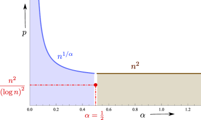
Figure 1: Envelope for the growth rates of $p$ for a nondegenerate limit law of the PEL ratio statistic. The smaller the $\alpha$, the stronger is the dependence.

The growth rate of $p$, for which a nondegenerate limit law holds for a suitably transformed $K_{n}$, primarily depends on the strength of dependence among the components of the observations; cf. Figure 1. In the NE-case, $p$ can grow arbitrarily fast (e.g., polynomial, exponential, super-exponential, etc.) as a function of $n$. In the E-case, although a degenerate limit law holds for an arbitrary growth rate of $p$, for a nondegenerate limit, $p$ must admit a suitable upper bound. In particular, for the Normal limit in the E-case (excluding the boundary case), the growth rate of $p$ as a function of $n$ is $p=o(n^{2})$. For the non-Normal limit under the E-case, $p=o(n^{1/\alpha})$ for $0<\alpha<1/2$ where, roughly speaking, $\alpha$ denotes the exponent of the rate of decay of the autocorrelation among the components of $X_{1}$, up to a permutation; cf. condition (C.4)_α, Section 3. The boundary case is given by $\alpha=1/2$, where the growth rate is slightly smaller and is given by $p=o(n/[\log n]^{2})$. From Figure 1, it follows that the stronger the dependence among the components of the observations, the higher is the allowable growth rate of $p$ as a function of $n$ for a nondegenerate limit. The limiting case $\alpha\rightarrow 0+$ is the NE-case. Here the nondegenerate limit for the the negative logarithm of the PEL ratio statistic holds for an arbitrary growth rate of $p$ as a function of $n$.

It is worth pointing out that in most cases, the limit distribution of the PEL ratio statistic is not distribution free in the sense that the asymptotic approximation to the distribution of the PEL ratio statistic requires the knowledge of one or more unknown population parameters. As a result, the limit laws are not directly usable in practice. To address this issue, we propose a calibration procedure based on the subsampling method. We show that under mild conditions, the subsampling based calibration method is consistent under all three types of dependence structures.

The key step in the proofs is to derive a quadratic asymptotic approximation to $K_{n}$ under all three cases of dependence. This is presented in Lemma 6.2 for the NE-case and in the proof of Theorem 3.2 for the E-case. The derivation of the limit law in the NE-case uses some weak convergence and operator convergence results on Hilbert spaces. On the other hand, in the E-case, refined approximations to $K_{n}$ are required to go beyond their degenerate limits. See Section 6 for more details.

The rest of the paper is organized as follows. In Section 2, we describe the PEL methodology. In Section 3, we introduce the asymptotic framework and establish the limit distributions of the logarithm of the PEL ratio statistic under the three dependence scenarios. In Section 4, we describe the subsampling method and prove its validity for all three cases. We report the results from a moderately large simulation study in Section 5. Proofs of the results are given in Section 6.

2 Formulation of the PEL

Let $X_{1},\ldots,X_{n}$ be i.i.d. random vectors with mean $\mu\in\mathbb{R}^{p}$. Let $X_{ij}$ denote the $j$th component of $X_{i}$, $1\leq i\leq n$, $1\leq j\leq p$. Also, let $A^{\prime}$ denote the transpose of a matrix $A$. We define the penalized empirical likelihood (PEL) of a plausible value $\mu=(\mu_{1},\ldots,\mu_{p})^{\prime}$ of the population mean as

$$L_{n}(\mu)=\sup_{(\pi_{1},\ldots,\pi_{n})^{\prime}\in\Pi_{n}}\Biggl{\{}\Biggl{(}\prod_{i=1}^{n}\pi_{i}\Biggr{)}\exp\Biggl{(}-\lambda\sum_{j=1}^{p}\delta_{j}\Biggl{[}\sum_{i=1}^{n}\pi_{i}(X_{ij}-\mu_{j})\Biggr{]}^{2}\Biggr{)}\Biggr{\}},$$ (1)

where $\Pi_{n}=\{(\pi_{1},\ldots,\pi_{n})^{\prime}\in[0,1]^{n}$ : $\sum_{i=1}^{n}\pi_{i}=1\}$, $\delta_{j}$’s are component specific weights (which may be random), and $\lambda=\lambda_{n}\in[0,\infty)$ is an overall penalty factor. Here we use

$$\delta_{j}\equiv\delta_{nj}=s_{nj}^{-2}\mathbh{1}(s_{nj}\neq 0),$$ (2)

where $s_{nj}^{2}=n^{-1}\sum_{i=1}^{n}(X_{ij}-\bar{X}_{nj})^{2}$ is the sample variance of the $j$th components of $X_{1},\ldots,X_{n}$, $\bar{X}_{nj}=n^{-1}\sum_{i=1}^{n}X_{ij}$ and where $\mathbh{1}(\cdot)$ denotes the indicator function. This choice of the component-wise scaling allows us to adjust for the heteroscedasticity along different co-ordinates of $X_{1}$ and therefore, the overall penalization parameter $\lambda$ gives comparable weights to all components. In addition, the choice of the penalty function makes the proposed PEL invariant with respect to component-wise scaling, which is an inherently desirable property, particularly while dealing with high-dimensional variables, where the assumption of homoscedasticity among a large number of components is unrealistic. The maximizer of the product $\prod_{i=1}^{n}\pi_{i}$ in (1) without the penalty term is given by $\pi_{i}=1/n$ for $i=1,\ldots,n$. Hence, the PEL ratio statistic at a plausible value $\mu$ of the mean vector is defined as

$$R_{n}(\mu)=n^{n}L_{n}(\mu).$$

We now compare our formulation with the PEL of Bartolucci (2007), which is defined as

$$\qquad L^{\mathrm{B}}_{n}(\mu)=\sup_{(\pi_{1},\ldots,\pi_{n})^{\prime}\in\Pi_{n}}\Biggl{\{}\Biggl{(}\prod_{i=1}^{n}\pi_{i}\Biggr{)}\exp\biggl{(}-\frac{n(v-\mu)^{\prime}V_{n}^{\dagger-1}(v-\mu)}{2h^{2}}\biggr{)}\Biggr{\}},$$ (3)

where $v=\sum_{i=1}^{n}\pi_{i}X_{i}$, $V_{n}^{\dagger}=n^{-1}\sum_{i=1}^{n}(X_{i}-\bar{X}_{n})(\bar{X}_{i}-\bar{X}_{n})^{\prime}$ is the sample covariance matrix, and $h$ is a penalty parameter. Note that for a large $p\in(1,n]$, the sample variance matrix $V_{n}$ is ill-conditioned, if the smallest eigen-value of the underlying covariance matrix $\Sigma$ (say) of $X_{1}$ is not bounded away from zero, and it is always singular when $p>n$, requiring further modifications to make (3) well defined. Under either of the two scenarios, the PEL based on (3) can be computationally demanding and unstable. In comparison, the component-wise scaling in (1) only involves $1$-dimensional operations which is computationally much simpler and feasible even for a large $p$. A second limitation of (3) is the lack of attractive theoretical properties of $V_{n}^{-1}$ (or of its variants) in high dimensions. Indeed, consistency of the sample covariance matrix (and its banded or tapered versions) in the high-dimensional setting is questionable in presence of strong correlations among the components of $X_{1}$ that we consider here. Existing work on consistency of the sample covariance matrix is known only under suitable conditions of sparsity or weak dependence; cf. Bickel and Levina (2008), El Karoui (2008), Cai, Zhang and Zhou (2010). Our formulation also avoids this problem altogether by using component-wise scaling.

For the sake of completeness, we also briefly describe the penalized EL approach of Otsu (2007) and Tang and Leng (2010), specialized to the case of the mean parameter $\mu$ for simplicity of exposition. Let $L_{n}^{\mathrm{ST}}(\mu)=\sup\{\prod_{i=1}^{n}\pi_{i}\dvtx(\pi_{1},\ldots,\pi_{n})\in\Pi_{n},\sum_{i=1}^{n}\pi_{i}(X_{i}-\mu)=0\}$ denote the standard EL for $\mu$. Also, let $p_{\lambda}(\cdot)$ be a penalty function, such as the smoothly clipped absolute deviation (SCAD) penalty function of Fan and Li (2001). Then, the penalized EL considered by Otsu (2007) and Tang and Leng (2010) is of the form

$$L_{n}^{\mathrm{OTL}}(\mu)=L_{n}^{\mathrm{ST}}(\mu)\exp\Biggl{(}-n\sum_{j=1}^{p}p_{\lambda}(\mu_{j})\Biggr{)},$$ (4)

where $\mu=(\mu_{1},\ldots,\mu_{p})^{\prime}$. For the case of a more general parameter $\theta$ defined through a set of estimating equations, the formulation of Otsu (2007) and Tang and Leng (2010) replaces $L_{n}^{\mathrm{ST}}(\mu)$ in (4) by the corresponding version of the standard EL for $\theta$; cf. Qin and Lawless (1994). As a result, irrespective of the target parameter, since (4) is directly based on the standard EL, this formulation of the penalized EL also suffers from the same limitations as the standard EL. In particular, this approach also fails in high dimensions whenever $p>n/2$.

In the next section, we investigate theoretical properties of the proposed PEL method (1) under the dependence structures described in Section 1.

3 Limit distributions

3.1 General framework

We establish the limit distribution theory for the PEL ratio statistic in a triangular array set up, with $n$ denoting the variable driving the asymptotics. Thus, the vectors $X_{1},\ldots,X_{n}$ depend on $n$ as are their distributions and the dimension $p$. However, we often suppress the dependence on $n$ for simplicity of notation. The limit distribution of the PEL ratio statistic depends on the degree of dependence among the components of $X_{1},\ldots,X_{n}$. As stated in Section 1, we can broadly classify the dependence structure into two categories: (i) Non-Ergodic (NE) and (ii) Ergodic (E). In the NE-case, the dependence among the components of each $X_{i}$ is so strong [cf. condition (C.3) below] that even the law of large numbers fails. In this case, we show that under appropriate conditions, the PEL ratio statistic has a nondegenerate limit. In contrast, in the E-case, the corresponding limit is degenerate, and further centering and scaling are needed for nondegenerate limit laws which, in turn, depend the type of dependence (SRD or LRD). We begin with the NE-case.

3.2 Limit distribution for the nonergodic case

We need to introduce some notation at this stage. Let $\rho_{n}(j,l)$ denote the correlation between $X_{1j}$ and $X_{1l}$, $1\leq j,l\leq p$. Let $\sigma_{nj}^{2}=\operatorname{Var}(X_{1j})$ and $D^{X}_{nj}=\{x\in\mathbb{R}\dvtx P(X_{1j}=x)>0\}$, $1\leq j\leq p$, $n\geq 1$. Write $C$ to denote a generic constant in $(0,\infty)$. Also, for any two sequences $\{a_{n}\}_{n\geq 1}$ and $\{b_{n}\}_{n\geq 1}\in(0,\infty)$, write $a_{n}\sim b_{n}$ if $a_{n}/b_{n}\rightarrow 1$ as $n\rightarrow\infty$. Let $L^{2}[0,1]$ denote the set of all square integrable functions on $[0,1]$ (with respect to the Lebesgue measure on $[0,1]$), equipped with the inner product $\langle f,g\rangle=\int_{0}^{1}fg$, $f,g\in L^{2}[0,1]$. Let $\{\phi_{k}\dvtx k\in\mathbb{N}\}$ denote a complete orthonormal basis of $L^{2}[0,1]$, where $\mathbb{N}=\{1,2,\ldots\}$ denotes the set of all positive integers. For any (bounded) jointly measurable function $h\dvtx[0,1]^{2}\rightarrow\mathbb{R}$, define the operator $\Upsilon_{h}$ on $L^{2}[0,1]$ by $\Upsilon_{h}f=\int_{[0,1]}h(\cdot;u)f(u)\,du$ for $f\in L^{2}[0,1]$. For $x,y\in\mathbb{R}$, let $x\wedge y=\min\{x,y\}$.

We shall make use of the following conditions for deriving the limit distribution of $-\log R_{n}(\mu)$. The values of the integers $r$ and $s$ below will be specified later in the statements of the theorems.

1. [(C.3)]

2. (i) $\max\{E[\sigma_{nj}^{2}\delta_{j}]^{s}\dvtx 1\leq j\leq p\}=O(1)$ for a given $s\in\mathbb{N}$.

   1. [(ii)]

   2. $\limsup_{n\rightarrow\infty}\max\{P(X_{nj}=x)\dvtx x\in D^{X}_{nj},1\leq j\leq p\}<1$.

3. (i) For a given $r\in\mathbb{N}$, $\max\{E|X_{1j}|^{r}\dvtx 1\leq j\leq p\}<C.$

   1. [(ii)]

   2. $\lambda_{n}=c_{*}n/p$ for some $c_{*}\in(0,\infty)$.

4. There exists a correlation function $\rho_{0}(\cdot,\cdot)$ of a mean-square continuous process on $[0,1]$, and for each $n\geq 1$, there exists a permutation $\iota_{n}$ of $\{1,\ldots,p_{n}\}$ such that $\rho_{n}(j,l)=\rho_{0}(\frac{\iota_{n}(j)}{p},\frac{\iota_{n}(l)}{p})$. Further, with $c_{*}$ as in (C.2), $\rho_{0}(\cdot,\cdot)$ satisfies the following:

   1. [(iii)]

   2. $4c_{*}^{2}\int_{0}^{1}\int_{0}^{1}\rho_{0}^{2}(u,v)\,du\,dv<1$;

   3. $\sup\{|\rho_{0}(u+h_{1},v+h_{2})-\rho_{0}(u,v)|\dvtx|h_{1}|\leq\delta,|h_{2}|\leq\delta\}\leq g(\delta)H(u,v)$ for all $u,v,u+h_{1},v+h_{2}\in[0,1]$ for some function $g(\cdot)$ satisfying $g(\delta)\rightarrow 0$ as $\delta\downarrow 0$ and for some function $H(\cdot,\cdot)$ satisfying $\sum_{k\geq 1}\langle|\phi_{k}|,|\Upsilon_{H}\phi_{k}|\rangle<\infty;$

   4. $\sum_{k\geq 1}\langle\phi_{k},\Upsilon_{0}\phi_{k}\rangle$ converges, where $\Upsilon_{0}=\Upsilon_{h}$ with $h=\rho_{0}$.

We now briefly comment on the conditions. Condition (C.1)(i) is a moment condition on the scaled component-wise weights $\delta_{j}$’s and requires finiteness of the $s$th negative moment of the sample variance $s_{nj}^{2}$’s (scaled by the respective expected values $\sigma_{nj}^{2}$’s). This condition holds in the case of Gaussian $X_{ij}$’s whenever the the sample size $n>2s$. Condition (C.1)(ii) is a mild condition—it says that none of the $X_{ij}$’s take a single value with probability approaching one. This condition trivially holds if the components of $X_{1}$ are continuous and also in the discrete case, if the supports of $X_{1j}$’s contain at least two values with asymptotically nonvanishing probabilities. Condition (C.2)(i) is a moment condition that will be used with different values of $r$ in the main theorems of this section, while (C.2)(ii) specifies the growth rate of the penalty parameter for a nondegenerate limit of $-\log R_{n}(\mu_{0})$. However, unlike the standard usage of the penalty parameter in the context of variable selection, where different choices of the parameter lead to different sets of variables being chosen, here the key role of the penalty parameter is to stabilize the contribution from the sum of component-wise squared differences to the overall “likelihood” in (1). Finally, consider condition (C.3) that specifies the nonergodic structure of the $X_{i}$’s. Note that, up to a (possibly unknown) permutation of the co-ordinates, the components of $X_{1}$ are essentially correlated as strongly as the variables $W(t)$’s coming from a constant mean, mean-square continuous process $\{W(t)\dvtx t\in[0,1]\}$ (say) with covariance function $\rho_{0}(\cdot)$. In this case, the dependence among the variables $W(i/p)$ and $W(j/p)$, $1\leq i<j\leq p$ is so strong that the average $p^{-1}\sum_{j=1}^{p}W(j/p)$ may not converge to a constant as $p\rightarrow\infty$, as one would expect from the well-known ergodic theorems.

Under conditions (C.1)–(C.3), the limit distribution of the log-PEL ratio statistic is given by a stochastic integral, as shown by the following result.

Theorem 3.1

Let conditions (C.1), (C.2) and (C.3) hold with $s=4$ and $r=8$, let $\mu_{0}$ denote the true value of $\mu$ and let $p\rightarrow\infty$ as $n\rightarrow\infty$. Then

$$-\log R_{n}(\mu_{0})\rightarrow^{d}c_{*}\int_{0}^{1}\int_{0}^{1}\Lambda_{0}(u,v)Z(u)Z(v)\,du\,dv,$$ (5)

where $Z(\cdot)$ is a zero mean Gaussian process on $[0,1]$ with covariance function $\rho_{0}(\cdot)$ and where the function $\Lambda_{0}(\cdot,\cdot)$ is defined as

$$\Lambda_{0}(u,v)=\sum_{k=0}^{\infty}(-2)^{k}c_{*}^{k}\rho_{0}^{*(k)}(u,v),\qquad 0<u,v<1,$$ (6)

with $\rho_{0}^{*(0)}(u,v)=1$, $\rho_{0}^{*(1)}(u,v)=\rho_{0}(u,v)$ and for $k\geq 1$,

$$\rho_{0}^{*(k+1)}(u,v)=\int_{0}^{1}\cdots\int_{0}^{1}\Biggl{\{}\prod_{j=1}^{k-1}\rho_{0}(u_{j},u_{j+1})\Biggr{\}}\rho_{0}(u_{1},u)\rho_{0}(u_{k},v)\,du_{1}\cdots\,du_{k}.$$

For a general definition of a stochastic integral of the form (5), see Cramer and Leadbetter (1967). Note that under condition (C.3), by repeated application of the Cauchy–Schwarz inequality, for $k\geq 1$,

$$\sup_{u,v\in[0,1]}\bigl{|}\rho_{0}^{*(k+1)}(u,v)\bigr{|}\leq(1-\delta)^{k-1}[2c_{*}]^{-(k+1)}\qquad\mbox{for some }\delta\in(0,1),$$

and hence, the limiting stochastic integral is well defined.

Theorem 3.1 shows that under a suitable choice of the penalty parameter, namely, $\lambda=c_{*}n/p$, the negative log PEL ratio statistic has a nondegenerate limit distribution. Note that, unlike the standard version of the EL, we do not use the multiple $2$ before $-\log R_{n}(\mu_{0})$. This is a direct artifact of the additional penalty term that we use in the formulation of PEL. Also, unlike most high-dimensional problems where the validity of a large sample inference procedure breaks down beyond a certain (often exponential) rate of growth of $p$, the PEL and the associated limit distribution of $-\log R_{n}(\mu_{0})$ in the NE-case remains valid for arbitrary rate of growth of $p$ as a function of the sample size. Thus, in the NE-case, it is possible to carry out simultaneous hypothesis testing for a very large number of parameters even with a moderately large sample.

3.3 Limit distribution for the ergodic case

In the E-case, we shall make use of the following conditions, for $\alpha\in(0,\infty)$:

[(C.4)_α]

There exists a covariance function $\rho_{\alpha}(\cdot)$ on $\mathbb{Z}\equiv\{0,\pm 1,\pm 2,\ldots\},$ and for each $n\geq 1$, there exists a (possibly unknown) permutation $\iota_{n}$ of $\{1,\ldots,p_{n}\}$ such that $\rho_{\alpha}(k)\sim C|k|^{-\alpha}$ as $k\rightarrow\infty$ and

$$\sup_{1\leq j,l\leq p}\biggl{|}\frac{\rho_{n}(j,l)}{\rho_{\alpha}(\iota_{n}(j)-\iota_{n}(l))}-1\biggr{|}=o(1)\qquad\mbox{as }n\rightarrow\infty.$$

There exists a constant $C>0$ such that

$$\check{\varrho}_{n}(k)\leq Ck^{-\alpha}\qquad\mbox{for all }k\geq 1,n>C,$$

where $\check{\varrho}_{n}(\cdot)$ denotes the $\varrho$-mixing coefficient of the variables $\{\tilde{X}_{1j}\dvtx 1\leq j\leq p\}$, defined by $\check{\varrho}_{n}(k)=\sup\{|P(A\cap B)-P(A)P(B)|/\sqrt{P(A)P(B)}\dvtx A\in\mathcal{F}_{1}^{m},B\in\mathcal{F}_{m+k}^{p},1\leq m\leq p-k\}$. Here, $\mathcal{F}_{a}^{b}$ denotes the $\sigma$-field generated by $\{\tilde{X}_{1j}\dvtx a\leq j\leq b\}$, $1\leq a\leq b\leq p$, $\tilde{X}_{1j}=X_{1\tau(j)},$ and $\tau=\tau_{n}$ is the inverse of the permutation $\iota_{n}$ in (C.4)_α.

Condition (C.4)_α says that up to a (possibly unknown) permutation of the coordinates, the components of the $X_{i}$-vectors have a dependence structure that is asymptotically similar to the one given by $\rho_{\alpha}(\cdot)$. Note that the sum $\sum_{k=0}^{\infty}|\rho_{\alpha}(k)|$ diverges if and only if $\alpha\leq 1$, and therefore, we classify the dependence structure of the $X_{1}j$’s as LRD or SRD according to $\alpha\leq 1$ or $\alpha>1$, respectively; cf. Beran (1994). Condition (C.5)_α is a decay condition on the $\varrho$-mixing coefficient of the reordered variables $\{\tilde{X}_{1j}\dvtx 1\leq j\leq p\}$. Note that by (C.4)_α, the correlation coefficient between $\tilde{X}_{1j}$ and $\tilde{X}_{1k}$ is $\rho_{\alpha}(j-k)(1+o(1))$, and therefore, the re-ordered sequence $\{\tilde{X}_{1j}\dvtx 1\leq j\leq p\}$ behaves approximately like a stationary time series with the natural time-index $j$. Thus, condition (C.5)_α specifies the degree of dependence of the $X_{ij}$’s, up to a permutation that need not be known to the user.

3.3.1 Results under short-range dependence

The following result shows that the log-PEL ratio statistic in the SRD case converges to a Normal limit after a suitable centering and after scaling by the “standard factor” $p^{1/2}$.

Theorem 3.2

Let conditions (C.1), (C.2) and (C.4)_α, (C.5)_α hold for some $\alpha>1$, $s\geq 6,r\geq 12$. Let $\kappa^{2}=2c_{*}^{2}\sum_{k=0}^{\infty}\rho_{0}(k)^{2}$. Then, for $p=o(n^{2})$,

$$p^{1/2}\bigl{[}-\log R_{n}(\mu_{0})-c_{*}\bigr{]}\rightarrow^{d}N\bigl{(}0,\kappa^{2}\bigr{)}.$$ (7)

We now comment on Theorem 3.2. From the proof, it follows that the distribution of the log-PEL ratio statistic, for a given sample size, is close to the sum of $p$ weakly dependent chi-squared random variables with one degree of freedom. As a result, centering at 1 and scaling by $p^{1/2}$ yields a nondegenerate Normal limit. The effect of the weak dependence shows up in the variance of the limiting Normal distribution, which depends on the correlation structure of the components of $X_{1}$. It is worth noting that in the SRD case, one can use Normal critical points with an estimated variance to calibrate simultaneous tests of $p$ hypotheses using the EL.

Theorem 3.2 extends existing results on the EL in more than one direction. Hjort, McKeague and Van Keilegom (2009) and Chen et al. (2009) proved a version of the result (i.e., a Normal limit) for the standard log-EL ratio statistic in increasing dimensions with centering at 1 and scaling by $p^{1/2}$. In comparison, Theorem 3.2 relaxes the restriction on the dimension $p$ of the parameter $\mu$, by allowing it to grow faster than the sample size. This should be compared with the best available rate of $p=o(n^{1/2})$, obtained by Chen et al. (2009). Further, Theorem 3.2 covers a wide range of dependence structures of the components of $X_{1j}$’s which are not covered by the earlier results (e.g., here the minimum eigen-value of the covariance matrix of $X_{1}$ need not be bounded away from zero). However, the most important implication of Theorem 3.2 is that under SRD, the penalization step circumvents the limitation of the standard EL which is known to break down beyond the threshold $p\leq n/2$, as shown by Tsao (2004).

3.3.2 Results under long-range dependence

For $\alpha\in(0,1]$, the sum$\sum_{k=1}^{\infty}\rho_{0}(k)$ fails to converge absolutely, and we refer to this as the LRD case. Sums of LRD random variables are known to have either a Normal or a non-Normal limit, depending on the value of $\alpha$. The next result deals with the case where $\alpha$ can be very small, and the limit law is non-Normal. Further, the scaling also depends on the correlation decay parameter $\alpha$, as shown by Theorem 3.3. Let $\Gamma(\alpha)=\int_{0}^{\infty}t^{\alpha-1}e^{-t}\,dt$ and ${\iota}=\sqrt{-1}$.

Theorem 3.3

Let conditions (C.1), (C.2) and (C.4)_α, (C.5)_α hold for some $\alpha\in(0,\frac{1}{2})$, $s\geq 6$ and $r\geq 12$. If $p=o(n^{1/\alpha})$, then

$$p_{n}^{\alpha}\bigl{[}-\log R_{n}(\mu_{0})-c_{*}\bigr{]}\rightarrow^{d}W,$$ (8)

where $W$ is defined in terms of a bivariate Wiener–Itô integral with respect to the random spectral measure $\zeta$ of the Gaussian white noise process as

$$W=c_{*}\bigl{[}2\Gamma(\alpha)\bigr{]}^{-1}\int\frac{\exp({\iota}[x_{1}+x_{2}])-1}{{\iota}[x_{1}+x_{2}]}|x_{1}x_{2}|^{(\alpha-1)/2}\,d\zeta(x_{1})\,d\zeta(x_{2}).$$

Theorem 3.3 shows that under very strong dependence (i.e., for small values of $\alpha$) in the E-case, the log-PEL ratio statistic, with the same centering but a different scaling factor, has a nondegenerate limit distribution and the limit law is non-Normal. Further, the range $p$ for which the result holds is $p=o(n^{1/\alpha})$, which is a decreasing function of $\alpha$. Thus, the stronger the dependence among the co-ordinates of $X_{1j}$’s, the larger is the allowable growth rate of $p$ as a function of $n$ for the validity of the limit distribution.

Theorems 3.2 and 3.3 exhaust the types of limit laws for the log-PEL ratio statistic in the E-case. However, in terms of the rate of decay of the correlation function, these leave out the case where $\alpha\in[1/2,1]$. Although $\alpha\in[1/2,1]$ corresponds to LRD in the traditional sense, the centered and scaled versions of the log-PEL ratio statistic continue to have a Normal limit as shown by the following result. Curiously, the scaling sequence as well as the growth rate of $p$ depend on whether $\alpha=1/2$ or $\alpha\in(1/2,1]$.

Theorem 3.4

Let conditions (C.1), (C.2) and (C.4)_α, (C.5)_α hold for some $1/2\leq\alpha\leq 1$, $s\geq 6,r\geq 12$. [(ii)]

If $1/2<\alpha\leq 1$ and $p=o(n^{2})$, then (7) holds.

If $\alpha=1/2$ and $p=o([n/\log n]^{2})$, then

$$[p\log p]^{1/2}\bigl{[}-\log R_{n}(\mu_{0})-c_{*}\bigr{]}\rightarrow^{d}N\bigl{(}0,c_{*}^{2}\bigr{)}.$$ (9)

Thus, it follows from Theorem 3.4 that the log-PEL ratio statistic is asymptotically Normal for all $\alpha\geq 1/2$, although the components of $X_{i}$’s have LRD when $\alpha\in[1/2,1]$. The peculiar behavior of the scaling sequence at the boundary value $\alpha=1/2$ is essentially determined by the growth rate of the series $\sum_{j=1}^{p}\rho_{\alpha}^{2}(j)$ as $p\rightarrow\infty$, which is asymptotically equivalent to $\log p$ for $\alpha=1/2$ but it is bounded for $\alpha>1/2$.

Remark 3.1.

Proofs of Theorems 3.2–3.4 show that for any $p\rightarrow\infty$, $-\log R_{n}(\mu_{0})\rightarrow_{p}c_{*}\mbox{ as }n\rightarrow\infty$, that is, the log-PEL ratio statistic has a degenerate limit under all sub-cases of the E-case, for arbitrarily large $p$ as a function of $n$. However, for nondegenerate limits, refined approximations to the difference $[-\log R_{n}(\mu_{0})-c_{*}]$ are needed. Here, we are able to show that an approximation of the form

$$-\log R_{n}(\mu_{0})-c_{*}=T_{n}+E_{n}$$ (10)

holds for all sub-cases of the E-case, where $T_{n}$ is a centered sum and where $E_{n}$ is an error term, roughly of the order of $O_{p}(n^{-1})$. Further, $T_{n}$ has a nondegenerate limit up to a suitable scaling, as a function of $p$, depending on the dependence structure of the $X_{1j}$’s. The bounds on the growth rate of $p$ in the different sub-cases of the E-case are then determined by the requirement that the scaled error term be asymptotically negligible. For example, in the SRD case, $p^{1/2}T_{n}\rightarrow^{d}N(0,\kappa^{2})$ and hence, $p^{1/2}E_{n}\rightarrow_{p}0$ if and only if $p^{1/2}/n\rightarrow 0$, which is equivalent to the bound $p=o(n^{2})$. Similar considerations lead to the respective upper bounds in the other sub-cases of the E-case.

Remark 3.2.

It is worth pointing out that the PEL can be used for constructing “conservative” large sample simultaneous tests of the $p$ hypotheses $H_{0}\dvtx\mu=\mu_{0}$ for arbitrarily large $p$ in the E-case. Indeed, for $p$ growing faster than the upper bounds given in Theorems 3.2–3.4, a conservative large sample simultaneous test of $H_{0}\dvtx\mu=\mu_{0}$ rejects $H_{0}$ if $|c_{*}+\log R(\mu_{0})|>n^{-1}\log n$. Note that by (10), this test attains the ideal level $0$ asymptotically.

4 A subsampling based calibration

In this section, we describe a nonparametric calibration method based on subsampling to approximate the quantiles of the nondegenerate limit laws in both E- and NE-cases, which typically involve unknown population parameters and hence, cannot be used directly in practice. Let $\mathcal{X}_{n}(I)=\{X_{i}\dvtx i\in I\}$ be a subset of $\{X_{1},\ldots,X_{n}\}$ where $I\subset\{1,\ldots,n\}$ is of size $m$ and where $1<m<n$ (specific conditions on $m$ are given below). On each $\mathcal{X}_{n}(I)$, we employ the PEL method and obtain a version of the PEL ratio statistic $R^{*}_{m}(\mu;I)$, by replacing $n$ with $m$ and $X_{1},\ldots,X_{n}$ by $\mathcal{X}_{n}(I)$ in the definitions $R_{n}(\mu)$. First consider the NE case. Here, the subsampling estimator of the distribution function $G_{n}^{\mathrm{NE}}(\cdot)\equiv P(-\log R_{n}(\mu_{0})\leq\cdot)$ under the null hypothesis $H_{0}\dvtx\mu=\mu_{0}$ is given by

$$\hat{G}_{n}^{\mathrm{NE}}(x)=|\mathcal{I}_{n}|^{-1}\sum_{I\in\mathcal{I}_{n}}\mathbh{1}\bigl{(}-\log R^{*}_{m}(\mu_{0};I)\leq x\bigr{)},\qquad x\in\mathbb{R},$$

where $\mathcal{I}_{n}$ is a collection of subsets of $\{1,\ldots,n\}$ of size $m$ and where $|A|$ denotes the size of a set $A$. All possible subsets of size $m$ cannot be used mainly due to the sheer number of such sets, and hence, only a small fraction of these subsets are used to compute $\hat{G}_{n}^{\mathrm{NE}}(\cdot)$ in practice. In view of the block resampling methods for time series data, here we shall take $\mathcal{I}_{n}$ to be the collection of all overlapping blocks (subsets) of size $m$ contained in $\{1,\ldots,n\}$. Then, we have the following result in the NE case.

Theorem 4.1

Suppose that the conditions of Theorem 3.1 hold and that

$$m^{-1}+m/n=o(1)\qquad\mbox{as }n\rightarrow\infty.$$ (11)

Then, $\sup_{x\in\mathbb{R}}|\hat{G}_{n}^{\mathrm{NE}}(x)-G_{n}^{\mathrm{NE}}(x)|\rightarrow_{p}0\mbox{ as }n\rightarrow\infty.$

Next consider the E-case. Note that for $\alpha=1/2$, the limit of the log-PEL ratio statistic is $N(0,1)$, which is distribution free. One can carry out a simple test [cf. Beran (1994)] to ascertain if “$H\dvtx\alpha=1/2$” is true and then use the limit distribution directly to conduct the PEL test of the simultaneous $p$ hypotheses $H_{0}\dvtx\mu=\mu_{0}$ using the $N(0,1)$ critical points, without the need for an alternative calibration. As a result, we concentrate on the values of $\alpha\neq 1/2$ in the E-case. Let ${\hat{\alpha}}_{n}$ be an estimator of the correlation parameter $\alpha$; cf. Remark 4.1 below. Let $R_{m}^{*}(\mu_{0};I)$ denote the PEL ratio statistic based on the subsample $\mathcal{X}(I)$ under $\mu_{0}$, and define

$$V^{*}_{m}(I)={\hat{b}}_{n}\bigl{[}-\log R_{m}^{*}(\mu_{0};I)-c_{*}\bigr{]},\qquad I\in\mathcal{I}_{n},$$

where ${\hat{b}}_{n}=p^{{\hat{\alpha}}_{n}\wedge{1}/{2}}$. Then, a subsampling estimator of the distribution of $V_{n}\equiv{\hat{b}}_{n}[-\log R_{n}(\mu_{0})-c_{*}]$ is given by $\hat{G}_{n,\alpha}(x)=|\mathcal{I}_{n}|^{-1}\sum_{I\in\mathcal{I}_{n}}\mathbh{1}(-\log V^{*}_{m}(I)\leq x),x\in\mathbb{R}$ and we have the following results.

Theorem 4.2

Suppose that there exists a $c_{0}\in\mathbb{R}$ such that

$$(\log p)[{\hat{\alpha}}-\alpha]\rightarrow_{p}c_{0}\qquad\mbox{as }n\rightarrow\infty.$$ (12)

[(ii)]

For $\alpha\in(1,\infty)$, let the conditions of Theorem 3.2 and for $\alpha\in(1/2,1]$, let those of Theorem 3.4(i) hold. If $p/m^{2}+m/n=o(1)$, then

$$\sup_{x\in\mathbb{R}}\bigl{|}\hat{G}_{n,\alpha}(x)-P(V_{n}\leq x)\bigr{|}\rightarrow_{p}0\qquad{\mbox{as }}n\rightarrow\infty.$$ (13)

If the conditions of Theorem 3.3 hold for some $\alpha\in(0,1/2)$ and $p^{\alpha}/m+m/n=o(1)$, then (13) holds.

Theorem 4.2 shows that for both Normal and non-Normal limit laws under the E-case, the subsampling method provides a valid approximation to the distribution of the log-PEL ratio statistic. Hence, one can use the quantiles of the subsampling estimators to calibrate simultaneous tests on $\mu$ in a unified manner. This is specially important in the case of non-Gaussian limit laws for which the quantiles are difficult to derive. However, for $\alpha>1/2$, the limit distribution is Gaussian, and an alternative approximation can be generated by using a Normal distribution with an estimated variance. Indeed, the latter may be preferable to subsampling from the computational point of view.

Remark 4.1.

In practice, the value of $\alpha$ is not known and must be estimated. First consider the case where the permutation $\iota_{n}(\cdot)$ in (C.4)_α is known. Then, we are essentially dealing with $n$ i.i.d. copies of a time series of length $p$ as observations. By using the $n$ replicates of the time series, it is easy to modify standard estimators of $\alpha$ based on a single time series [cf. Beran (1994)] to construct an estimator ${\hat{\alpha}}$ of $\alpha$ satisfying ${\hat{\alpha}}-\alpha=o_{p}(n^{-1/2}[\log p]^{-1})\mbox{ as }n\rightarrow\infty$, which clearly satisfies (12) with $c_{0}=0$.

Next consider the case where the permutations $\iota_{n}(\cdot)$ are unknown. In this case, it is not possible to identify pairs $(j,l)$, $1\leq j,l\leq p$ that correspond to the lag-$k$ correlation $\rho_{\alpha}(k)$. However, it is still possible to construct estimators of $\alpha$ that satisfy (12). Define

$${\hat{\alpha}}=-(\log p)^{-1}\log\Biggl{(}e_{n}+n^{-1}\sum_{i=1}^{n}\Biggl{\{}p^{-1}\sum_{j=1}^{p}[X_{ij}-\bar{X}_{nj}]\delta_{j}^{1/2}\Biggr{\}}^{2}\Biggr{)},$$ (14)

where $e_{n}=\prod_{j=1}^{p}\mathbh{1}(s_{nj}=0)$ and $\delta_{j}$ (and $\bar{X}_{nj}$ and $s_{nj}$) are as in (2). Note that ${\hat{\alpha}}$ is invariant under permutations of the components of $X_{i}$’s and also under component-wise location and scale transformations. In Section 6, we show that ${\hat{\alpha}}$ satisfies (12) under the conditions of Theorem 4.2, even when $\iota_{n}(\cdot)$ is unknown. In the same spirit, we may use the following estimator of the limiting variance $\kappa^{2}$ in Theorem 3.2 in the case where $\iota_{n}(\cdot)$ is unknown:

$$\hat{\kappa}^{2}=2c_{*}^{2}\sum_{j=2}^{p-1}\hat{c}(1,j)^{2}\mathbh{1}\bigl{(}\bigl{|}\hat{c}(1,j)\bigr{|}>2n^{-1/2}\log n\bigr{)},$$ (15)

where $\hat{c}(j,k)=n^{-1}\sum_{i=1}^{n}(X_{ij}-\bar{X}_{nj})(X_{kn}-\bar{X}_{nk})\delta_{j}\delta_{k}$, $1\leq j,k\leq p$. Consistency of $\hat{\kappa}^{2}$ holds under mild moment conditions; cf. Section 6.

Remark 4.2.

An important factor that impacts the accuracy of the subsampling method is the choice of the subsample size $m$. Note that

$$m=C[np]^{\alpha_{0}/(1+\alpha_{0})}$$ (16)

satisfies the requirements of Theorem 4.2, where $\alpha_{0}=\min\{\alpha,1/2\}$. At this point, we do not know the order of the optimal $m$ for the different cases considered here. In the next section, we address this through a numerical study and explore the effects of different choices of $m$ on the performance of the PEL method.

5 Numerical study

We assess finite sample performance of the PEL method by simulation in a variety of settings. We considered different combinations of the sample size $n$ and the dimension $p$, with $p\approx 2n^{1/3},n/2,2n$ and $n=40$ and $200$. The testing problem we considered is $H_{0}\dvtx\mu=0$, although any other value of $\mu$ may be used in $H_{0}$, as the PEL criterion is location invariant. We generated i.i.d. random $p$-vectors $X_{1},\ldots,X_{n}$ where the $p$ coordinates of $X_{i}$’s had one of the three different types of dependence structures, namely: (i) non-Ergodic, (ii) LRD and (iii) SRD, as follows.

5.1 Algorithms for generating the data

5.1.1 The nonergodic case

[(1)]

Consider the basis functions in $L^{2}[0,1]$ given by $\phi_{j}(t)=\sin{(2\pi jt)}/\sqrt{2}$ for $j=1,2,\ldots,15$ and $\phi_{j}(t)=\cos{(2\pi(j-15)t)}/\sqrt{2}$, for $j=16,2,\ldots,30$ and $\phi_{0}(t)\equiv 1$.

Generate $Z_{j}\sim\rm{N}(0,1)$ i.i.d. and let $\lambda_{j}=(\exp{\{1\}}+1)$ for all $j$.

Define $X_{1j}=\sigma_{j}\cdot W(j/p),j=1,2,\ldots,p$, where $W(\cdot)=\sum_{j=0}^{30}Z_{j}\phi_{j}({\cdot})\lambda_{j}$ and where $\sigma_{j}\equiv\sigma_{jn}$ are scalars in $(0,\infty)$. Then, $X_{1}=\{X_{11},X_{12},\ldots,X_{1p}\}$ is a nonergodic series. Replicates of $X_{1}$ yield $X_{1},\ldots,X_{n}$ in the NE-case.

5.1.2 Long-range dependence

For the LRD case, we follow a setup similar to that used in Hall, Jing and Lahiri (1998). We generate stationary increments of a self-similar process with self-similarity parameter (or Hurst constant) $H=\frac{1}{2}(2-\alpha)\in(1/2,1)$ for $\alpha\in(0,1)$. The algorithm is as follows: [(1)]

Generate a random sample $\textbf{Z}_{p0}=\{Z_{10},\ldots,Z_{p0}\}$ from $N(0,1)$.

Define ${\bf Z}_{p}\equiv U^{T}{\bf Z}_{p0}$, where $U$ is obtained by Cholesky factorization of $R$ into $R=U^{T}U$ and where $R=((r_{ij}))$ with $r_{ij}=\rho_{\alpha}(|i-j|)$, and

$$\rho_{\alpha}(k)=\tfrac{1}{2}\bigl{\{}(k+1)^{2H}+(k-1)^{2H}-2k^{2H}\bigr{\}},\qquad k\geq 1,$$ (17)

and $\rho_{\alpha}(0)=1$. Note that $\rho_{\alpha}(k)\sim Ck^{-\alpha}\rm{as}k\rightarrow\infty$.

Replicates of $\textbf{Z}_{p}$ give the variables $X_{1},\ldots,X_{n}$ in the LRD case.

For the simulation study here, we considered the NE-case ($\alpha=0$) where the data were generated by the algorithm in Section 5.1.1 and the LRD cases $\alpha=0.1$ and $0.8$ based on the algorithm of Section 5.1.2. For the SRD case ($\alpha=\infty$), $X_{1}$ was generated by an $\operatorname{ARMA}(2,3)$ process with $N(0,1)$ error variables and parameter vector $(-0.4,0.1;0.3,0.5,0.1)$.

5.2 Choice of the subsample size

We also considered different choices of the subsample size $m$ in order to get some insight into its effects on the accuracy of the subsampling calibration. Note that the feasible choices of the subsample size depend on the relative growth rates of both $n$ and $p$ as well as on the strength of dependence, here quantified by $\alpha$. For each pair $(p,n)$, we considered three choices of the subsample size $m$ (denoted by the generic symbols $m_{1},m_{2},m_{3}$), depending on the dependence structure. Specifically, for the SRD case ($\alpha=\infty$), we set

$$m_{i}=c_{i}^{0}\cdot[np]^{1/3},\qquad i=1,2,3,$$

where $c_{1}^{0}=0.5$, $c_{2}^{0}=1$ and $c_{3}^{0}=2$. Note that in this case, the random variables in $X_{1},\ldots,X_{n}$ form a series of length $np$ and are weakly dependent. Further, the target parameter for the subsampling method in the SRD case (and also in the LRD case with $\alpha>1/2$) is the variance of the limiting Normal distribution. Hence, in view of the well-known results on optimal block length (for variance estimation) [cf. Hall, Horowitz and Jing (1995), Lahiri (2003)], the above choices of the $m_{i}$’s are reasonable.

Table 1: Empirical levels of significance $\hat{a}$ for the subsampling based PEL, with sample size $n=200$ at $0.05$ significance level and $c_{*}=1$. Here we have reported $|0.05-\hat{a}|$

	$\bolds{p_{1}=20}$			$\bolds{p_{2}=100}$			$\bolds{p_{3}=400}$
$\bolds{\alpha}$	$\bolds{m_{1}}$	$\bolds{m_{2}}$	$\bolds{m_{3}}$	$\bolds{m_{1}}$	$\bolds{m_{2}}$	$\bolds{m_{3}}$	$\bolds{m_{1}}$	$\bolds{m_{2}}$	$\bolds{m_{3}}$
$0.0$	0.0092	0.0063	0.0190	0.0090	0.0114	0.0162	0.0089	0.0103	0.0091
$0.1$	0.0099	0.0081	0.0171	0.0045	0.0069	0.0129	0.0149	0.0134	0.0094
$0.8$	0.0079	0.0031	0.0061	0.0086	0.0042	0.0081	0.0101	0.0099	0.0190
$\infty$	0.0059	0.0091	0.0010	0.0020	0.0104	0.0039	0.0091	0.0159	0.0078

Table 2: Empirical levels of significance $\hat{a}$ for the subsampling based PEL, with sample size $n=200$ at $0.1$ significance level and $c_{*}=1$. Here we have reported $|0.1-\hat{a}|$

	$\bolds{p_{1}=20}$			$\bolds{p_{2}=100}$			$\bolds{p_{3}=400}$
$\bolds{\alpha}$	$\bolds{m_{1}}$	$\bolds{m_{2}}$	$\bolds{m_{3}}$	$\bolds{m_{1}}$	$\bolds{m_{2}}$	$\bolds{m_{3}}$	$\bolds{m_{1}}$	$\bolds{m_{2}}$	$\bolds{m_{3}}$
$0.0$	0.170	0.020	0.075	0.221	0.142	0.090	0.075	0.152	0.227
$0.1$	0.030	0.033	0.033	0.012	0.005	0.011	0.112	0.133	0.066
$0.8$	0.011	0.045	0.087	0.123	0.082	0.018	0.108	0.027	0.069
$\infty$	0.138	0.135	0.065	0.050	0.011	0.003	0.048	0.054	0.026

Next consider the case $\alpha=0.1$ under LRD, where the limit distribution is non-Normal. From the proofs of Theorems 3.2 and 4.2, it follows that the prescription for $m$ in (16) attempts to balance the bias of the subsampling approximation to the limit distribution and its variance. However, for a very small value of $\alpha$, a direct application of (16) leads to a very small fractional exponent of $np$, which may be too small in practice. In such situations, particularly where $p$ is not very large and the LRD exponent $\alpha$ is small, we use the threshold $n^{1/3}$ and set

$$m_{i}\equiv m_{i}(\alpha)=c_{i}^{0}\cdot\max\bigl{\{}[np]^{\alpha/(1+\alpha)},n^{1/3}\bigr{\}},\qquad i=1,2,3,$$

where $c_{i}^{0}$’s are as before. The rationale behind this modification is that for $p$ small, we simply treat $X_{1},\ldots,X_{n}$ as a weakly dependent multivariate time series and again employ the known results on the optimal block size.

Finally, consider the NE-case, $\alpha=0$. Note that for $\alpha=0$, $p$ can grow at an arbitrary rate with the sample size $n$ for the validity of Theorems 3.1 and 4.1. Hence, in this case, our choice of $m$ depends only on the sample size. We consider the “canonical” choice $m_{1}=n^{1/3}$ as well as the larger values $m_{2}=n^{1/2}$ and $m_{3}=2n^{1/2}$ to explore the effects of a larger subsample size on the accuracy of the subsampling calibration method.

5.3 Results

5.3.1 Levels of significance in simultaneous tests

Here we consider finite sample accuracy of the proposed PEL method for simultaneous testing of the $p$ hypotheses

$$H_{0}\dvtx\mu=0\quad\mbox{vs.}\quad\mu\neq 0$$ (18)

at the levels of significance $a=0.1,0.05$. The correlation parameter $\alpha$ for the subsampling based calibration was estimated by averaging the Taqqu, Teverovsky and Willinger (1995) estimator of the Hurst parameter ($H$) from each of the $p$-time series and by setting $\hat{\alpha}=(2-2\hat{H})$. Further, we have used the interior-point method [cf. Wright (1997)] as a fast optimization tool for computing the PEL ratio statistic, which can handle high-dimensional optimization problems efficiently. Tables 1 and 2 report the attained levels of significance based on $500$ simulation runs and $n=200$ for the target significance levels of $0.05$ and $0.10$, respectively, for different values of $p$, $m$, and $\alpha$.

Table 3: Power of the proposed PEL, with sample size $n=200$ at $0.1$ significance level and $c_{*}=1$

	$\bolds{p_{1}=20}$			$\bolds{p_{2}=100}$			$\bolds{p_{3}=400}$
$\bolds{\alpha}$	$\bolds{m_{1}}$	$\bolds{m_{2}}$	$\bolds{m_{3}}$	$\bolds{m_{1}}$	$\bolds{m_{2}}$	$\bolds{m_{3}}$	$\bolds{m_{1}}$	$\bolds{m_{2}}$	$\bolds{m_{3}}$
$0.0$	0.569	0.681	0.929	0.515	0.643	0.791	0.870	0.834	0.766
$0.1$	0.660	0.710	0.850	0.569	0.903	0.676	0.794	0.800	0.868
$0.8$	0.515	0.883	0.688	0.750	0.997	0.488	0.700	0.870	0.900
$\infty$	0.510	0.622	0.870	0.739	0.778	0.996	0.802	0.790	0.939

From the tables, it follows that the PEL does a reasonable job of simultaneous testing of $p$ hypotheses for all $4$ cases of dependence, for appropriately chosen subsample size. Comparing the attained level of significance, it is clear that the best choice of the subsample size critically depends on the relative sizes of $n$ and $p$, and more importantly, on the type of dependence among the components of $X_{1}$. Further, rather surprisingly, the PEL tests at the level of significance $0.05$ turned out to be more accurate (on an absolute scale) than at the level $0.1$, for the subsample sizes considered here.

We also considered the effect of the penalty parameter $\lambda_{n}=c_{*}n/p$ on the performance of the PEL test. In the supplementary material Lahiri and Mukhopadhyay (2012) (hereafter referred to as [LM]), we report the empirical levels of significance of the PEL test for $n=200$ and the target level $0.1$ for two other choices of the constant $c_{*}$, namely, $c_{*}=0.5$ and $c_{*}=2.0$. The results for the choice $c_{*}=2$ are qualitatively similar to those reported in Table 2 (with $c_{*}=1$); in comparison, the accuracy for the case $c_{*}=0.5$ appears to be slightly better than the $c_{*}=1$ case. A similar pattern was observed for the $0.05$ level of significance. We also considered the accuracy of the empirical significance levels of the PEL tests at a relatively smaller sample size $n=40$, for $c_{*}=1$ and $\alpha=0.1$; cf. [LM]. The PEL has a reasonable performance even at this low sample size; see [LM] for details.

5.3.2 Finite sample power properties

To get some idea about the power properties of the PEL tests, we computed the probability of Type II error for a level $0.1$ PEL test with $n=200$ and $c_{*}=1$ under the alternative $\mu=\mu_{1}$ where the first $p/2$ components of $\mu_{1}$ were equal to $1$ and the rest were $0$. Table 3 gives the power of the PEL test at level $0.1$ under $\mu=\mu_{1}$ for different combinations of $p$, $\alpha$ and $m$. From Table 3, it appears that the power can be reasonably high for a suitable choice of the subsample size, although the maximum value critically depends on the dimension $p$ of the parameters and the strength of dependence $\alpha$. In particular, the PEL attains a higher (maximum) power under weaker dependence ($\alpha=0.8,\infty$) than under strong dependence ($\alpha=0,0.1$).

5.3.3 Comparison with Normal calibration

Note that for $\alpha>1/2$, the limit distribution of the logarithm of the PEL ratio statistic is Normal and therefore, one can use the limiting Normal distribution with an estimated variance to conduct the PEL test. In this section, we compare the performance of the subsampling-based calibration with the Normal distribution-based calibration. To estimate the asymptotic variance $\kappa^{2}=2c_{*}^{2}\sum_{k=0}^{\infty}\rho_{0}(k)^{2}$, we first estimate $\rho_{0}(k)$ using the sample auto-covariance at lag-$k$ based on the components of individual $X_{i}$’s and then average them to get an estimate ${\hat{\rho}}_{n}(k)$ of $\rho_{0}(k)$ for $k=1,\ldots,K$ where $K=\min\{p/2,p^{1/2}\}$. Since $\kappa^{2}$ involves the squares of $\rho_{0}(k)$, the plug-in estimator is positive (with probability $1$). Tables 4 and 5 compare the best performance of the subsampling based PEL with the Normal, calibration-based PEL for $n=40$ and $n=200$, respectively.

Table 4: Comparison of the subsampling (SS) and Normal (G) calibrations for $n=40$

	$\bolds{p_{1}=7}$		$\bolds{p_{2}=20}$		$\bolds{p_{3}=80}$
$\bolds{\alpha}$	G	SS	G	SS	G	SS
$0.8$	0.122	0.151	0.132	0.080	0.136	0.081
$\infty$	0.098	0.092	0.030	0.111	0.076	0.093

Tables 4 and 5 show that, except for the small values of $p$, the subsampling-based PEL method has a better accuracy (marked as bold) than the Normal, calibration-based PEL. However, the computational burden associated with the subsampling method is typically larger than the Normal-based PEL.

Table 5: Comparison of the subsampling (SS) and Normal (G) calibrations for $n=200$

	$\bolds{p_{1}=7}$		$\bolds{p_{2}=20}$		$\bolds{p_{3}=80}$
$\bolds{\alpha}$	G	SS	G	SS	G	SS
$0.8$	0.150	0.113	0.141	0.082	0.174	0.127
$\infty$	0.111	0.165	0.048	0.103	0.238	0.126

6 Proofs

Note that for each $n\geq 1$, the PEL likelihood function in (1) is invariant with respect to (i) component-wise scaling and (ii) permutation of the $p$ components. Hence, all through this section, without loss of generality (w.l.g.), we set the component-wise variance $\sigma_{nj}^{2}=1$ and set the permutation $\iota_{n}(j)=j$ for all $1\leq j\leq p$ and $n\geq 1$. Let $C,C(\cdot)$ denote generic constants that depend only on their arguments (if any), but not on $n$. Unless otherwise specified, dependence on (limiting) population quantities [such as $\rho_{0}(\cdot)$, mixing coefficients, etc.] are dropped to simplify notation, and limits in all order symbols are taken by letting $n\rightarrow\infty$. For $x\in\mathbb{R}$, let $\lfloor x\rfloor$ denote the largest integer not exceeding $x$ and let $x_{+}=\max\{x,0\}$.

6.1 Limit distribution in the nonergodic case

Lemma 6.1

For each $n\geq 1$, let {$Y_{ij}=\mathrm{Y}_{ijn},1\leq j\leq p$}, $i=1,2,\ldots,n$ be a collection of $p=p_{n}$-dimensional random vectors with $\mathrm{E}Y_{1j}=0$ and $\mathrm{E}Y^{2}_{1j}=\sigma^{2}_{nj}\in(0,\infty)$. Let $\delta_{j}\equiv\delta_{nj}=s^{-2}_{nj}\mathbh{1}(s_{nj}\neq 0)$ where $s^{2}_{nj}={n^{-1}\sum_{i=1}^{n}}(Y_{ij}-\bar{Y}_{jn})^{2}$ and $\bar{Y}_{nj}={n^{-1}\sum_{i=1}^{n}}Y_{ij}$. Also, let $Z_{ij}=|Y_{ij}|-\mathrm{E}|Y_{ij}|,$ $\bar{Z}_{jn}={n^{-1}\sum_{i=1}^{n}}Z_{ij}$, $W_{i}(j,l)=Y_{ij}Y_{il}-EY_{ij}Y_{il}$, $\bar{W}_{n}(j,l)=n^{-1}\sum_{i=1}^{n}W_{i}(j,l)$ and $D_{jn}=\{y\in\mathbb{R}\dvtx\break P(Y_{1j}=y)>0\}$. Suppose that (L.1) $\max\{\mathrm{E}({\sigma^{2}_{nj}}{\delta_{j}})^{4}\dvtx 1\leq j\leq p\}=O(1)$; (L.2) $\max\{\mathrm{E}|Y_{ij}|^{8}\dvtx 1\leq j\leq p\}<\mathrm{C}$, and (L.3) $\limsup_{n\rightarrow\infty}$ $\max\{P(Y_{1j}=y)\dvtx y\in D_{jn},j=1,\ldots,p\}<1$. Then: [(a)]

For $k=1,2,3$, $\sum_{j=1}^{p}\delta_{j}\bar{Y}^{2k}_{jn}=O_{p}(n^{-k}p)$.

$\sum_{j=1}^{p}\delta_{j}[\bar{Z}_{jn}^{2}+\bar{W}^{2}_{jn}]=O_{p}(n^{-1}p)$.

$\sum_{j=1}^{p}\sum_{l=1}^{p}(\delta_{j}+1)\delta_{l}\bar{W}^{2}_{n}(j,l)=O_{p}(n^{-1}p^{2})$.

For $r=1,2$, $\max_{1\leq j\leq n}\sum_{j=1}^{p}\delta_{j}|\mathrm{Y}_{1j}|^{r}=O([pn]^{1/4})$.

$\sum_{j=1}^{p}(\delta_{j}-1)^{2}=O_{p}(n^{-1}p)$.

By replacing $Y_{ij}$’s with $Y_{ij}/\sigma_{nj}$ for all $i,j$, w.l.g., we can assume that $\sigma_{nj}=1$ for all $j,n$. First consider part (a), $k=3$; the proofs of $k=1,2$ are similar. By repeated use of Hölder’s inequality,

$$\mathrm{E}\sum_{j=1}^{p}\delta_{j}|\bar{Y}_{nj}|^{6}\leq\mathrm{E}\Biggl{(}\sum_{j=1}^{p}\delta_{j}^{4}\Biggr{)}^{1/4}\Biggl{(}\sum_{j=1}^{p}\bar{Y}_{nj}^{8}\Biggr{)}^{3/4}\leq\Biggl{(}\mathrm{E}\sum_{j=1}^{p}\delta_{j}^{4}\Biggr{)}^{1/4}\Biggl{(}\mathrm{E}\sum_{j=1}^{p}\bar{Y}_{nj}^{8}\Biggr{)}^{3/4},$$

which is $O(pn^{-3})$, by (L.1), (L.2). This proves (a). Parts (b) and (c) follow by similar arguments. As for part (d), note that (for $r=2$)

$$\mathrm{E}\Biggl{(}\max_{1\leq i\leq n}\sum_{j=1}^{p}\delta_{j}Y_{ij}^{2}\Biggr{)} \leq \Biggl{[}n\mathrm{E}\Biggl{(}\sum_{j=1}^{p}\delta_{j}Y_{1j}^{2}\Biggr{)}^{4}\Biggr{]}^{1/4}$$

$$\leq n^{1/4}\Biggl{[}\mathrm{E}\Biggl{(}\sum_{j=1}^{p}\delta_{j}^{4}\Biggr{)}^{1/4}\Biggl{(}\mathrm{E}\sum_{j=1}^{p}|Y_{1j}|^{8/3}\Biggr{)}^{3/4}\Biggr{]}^{1/4}\leq Cn^{1/4}p^{1/4}.$$

Finally consider part (e). Note that for $j=1,2,\ldots,p$

$$\delta_{j}-1 = \frac{1-s_{nj}^{2}}{s_{nj}^{2}}\mathbh{1}(s_{nj}\neq 0)-\mathbh{1}(s_{nj}=0)$$

$$= \delta_{j}\Biggl{[}\bar{Y}_{nj}^{2}-{n^{-1}\sum_{i=1}^{n}}\bigl{(}Y_{ij}^{2}-1\bigr{)}\Biggr{]}-\mathbh{1}(s_{nj}=0)$$

$$= \delta_{j}\bar{Y}_{nj}^{2}-\delta_{j}\overline{\mathrm{W}}_{n}(j,j)-\mathbh{1}(s_{nj}=0),$$

so that

$$\delta_{j}=\mathbh{1}(s_{nj}\neq 0)+\delta_{j}\bar{Y}_{nj}^{2}-\delta_{j}\overline{\mathrm{W}}_{n}(j,j).$$ (19)

Part (e) can now be proved using (L.1)–(L.3) and the Cauchy–Schwarz inequality. We omit the details to save space.

Lemma 6.2

Under the conditions of Theorem 3.1,

$$-\log{R}_{n}(\mu_{0})=n\gamma_{n}\biggl{(}\frac{\bar{Y}_{n1}}{\sigma_{n1}},\ldots,\frac{\bar{Y}_{np}}{\sigma_{np}}\biggr{)}(\mathrm{I}_{p}+2\gamma_{n}\mathrm{A}_{n})^{-1}\biggl{(}\frac{\bar{Y}_{n1}}{\sigma_{n1}},\ldots,\frac{\bar{Y}_{np}}{\sigma_{np}}\biggr{)}^{\prime}+o_{p}(1),$$

where $\bar{Y}_{nj}={n^{-1}\sum_{i=1}^{n}}Y_{ij}$, $Y_{ij}=X_{ij}-\mu_{j}$, $1\leq j\leq p,1\leq i\leq n$ and $\mathrm{A}_{n}=((\rho_{n}(i-j)))_{p\times p}$.

W.l.g., let $\sigma_{nj}=1$ for all $1\leq j\leq p,1\leq i\leq n$. Note that

$$-\log{R}_{n}(\mu_{0})=\min\bigl{\{}f(\pi_{1},\ldots,\pi_{n})\dvtx(\pi_{1},\ldots,\pi_{n})^{\prime}\in\Pi_{n}\bigr{\}},$$ (20)

where $f(\pi_{1},\ldots,\pi_{n})=-\sum_{i=1}^{n}\log(n\pi_{i})+\lambda_{n}\sum_{j=1}^{p}\delta_{j}(\sum_{i=1}^{n}\pi_{i}Y_{ij})^{2}$. Since $f(\cdot)$ is strictly convex in $\pi_{1},\ldots,\pi_{n}$ over a closed convex set $\Pi_{n}\subset\mathbb{R}^{n}$, it has a unique minimizer in $\Pi_{n}$. [The maximum of $f(\cdot)$ over $\Pi_{n}$ is $+\infty$.] To find the minimizer, we use a Lagrange multiplier $\eta$ and solve the set of equations

$$\frac{\partial}{\partial\pi_{k}}g(\pi_{1},\ldots,\pi_{n};\eta) = 0,\qquad 1\leq k\leq n,$$

$$\frac{\partial}{\partial\eta}g(\pi_{1},\ldots,\pi_{n};\eta) = 0,$$

where $g(\pi_{1},\ldots,\pi_{n};\eta)=\sum_{i=1}^{n}\log(n\pi_{i})-\lambda_{n}\sum_{j=1}^{p}\delta_{j}(\sum_{i=1}^{n}\pi_{i}Y_{ij})^{2}+\break\eta(\sum_{i=1}^{n}\pi_{i}-1)$. This leads to the equations

$${0}=\pi^{-1}_{k}-2\lambda_{n}\sum_{j=1}^{p}\delta_{j}\Biggl{(}\sum_{i=1}^{n}\pi_{i}Y_{ij}\Biggr{)}\mathrm{Y}_{kj}+\eta,\qquad 1\leq k\leq n\quad\mbox{and}\quad{1}=\sum_{i=1}^{n}\pi_{i},$$

which, in turn, yield the implicit solution

$$\eta = 2\lambda_{n}\sum_{j=1}^{p}\delta_{j}M_{nj}^{2}-n\quad\mbox{and}$$

$$\pi_{k}^{-1} = n\Biggl{\{}1+2\gamma_{n}\sum_{j=1}^{p}\delta_{j}M_{nj}\mathrm{Y}_{kj}-2\gamma_{n}\sum_{j=1}^{p}M_{nj}^{2}\delta_{j}\Biggr{\}},\qquad 1\leq k\leq n,$$

where $\gamma_{n}=\lambda_{n}/n$ and $M_{nj}=\sum_{i=1}^{n}\pi_{i}Y_{ij}$. To obtain a more explicit approximation, we show that $\pi_{k}$’s are of the form $\pi_{k}=n^{-1}(1+o_{p}(1))$ uniformly in $k$. In view of Brouwer’s fixed point theorem [cf. Milnor (1965)], it is enough to show that, with $a_{n}^{-1}=n^{-1/2}\log(n)$,

$$\max_{1\leq k\leq n}\Biggl{|}\frac{1}{n}\Biggl{\{}1+2\gamma_{n}\sum_{j=1}^{p}\delta_{j}M_{nj}\mathrm{Y}_{kj}-2\gamma_{n}\sum_{j=1}^{p}M_{nj}^{2}\delta_{j}\Biggr{\}}^{-1}-\frac{1}{n}\Biggr{|}$$

(22)

$$\qquad=O_{p}\bigl{(}n^{-1}a_{n}^{-1}\bigr{)}$$

whenever $\max\{|\pi_{k}-n^{-1}|\dvtx 1\leq k\leq n\}=O(n^{-1}a_{n}^{-1})$. To prove (6.1), we first show that

$$\sup\Biggl{\{}\gamma_{n}\sum_{j=1}^{p}\delta_{j}\mathrm{M}^{2}_{nj}\dvtx(\pi_{1},\ldots,\pi_{n})^{\prime}\in\Pi^{0}_{n}\Biggr{\}}=O_{p}\bigl{(}a_{n}^{-2}\bigr{)},$$ (23)

where $\Pi^{0}_{n}=\{(\pi_{1},\ldots,\pi_{n})^{\prime}\in\Pi_{n}\dvtx|\pi_{k}-n^{-1}|\leq Ca_{n}^{-1}n^{-1}$ for all $1\leq k\leq n\}$. Note that for any $(\pi_{1},\ldots,\pi_{n})^{\prime}\in\Pi^{0}_{n},\sum_{i=1}^{n}\pi_{i}=1=\sum_{i=1}^{n}(1/n)$ $\Longrightarrow\sum_{i=1}^{n}(1-n\pi_{i})=0\Longrightarrow\sum_{i}(1-n\pi_{i})_{+}=\sum_{i}(n\pi_{i}-1)_{+}$. Also, $(n\pi_{i}-1)_{+}>0$ if and only if (iff) $n\pi_{i}>1$ and similarly, $(1-n\pi_{i})_{+}>0$ iff $n\pi_{i}<1$. Hence, using the bound “$|n\pi_{i}-1|\leq\mathrm{C}a_{n}^{-1}$ for all $i=1,\ldots,n$,” we have

$$\Biggl{|}\sum_{i=1}^{n}(n\pi_{i})^{-1}-n\Biggr{|} = \Biggl{|}\sum_{i=1}^{n}\frac{(1-n\pi_{i})_{+}}{n\pi_{i}}-\sum_{i=1}^{n}\frac{(n\pi_{i}-1)_{+}}{n\pi_{i}}\Biggr{|}$$

$$= \Biggl{|}\sum_{i=1}^{n}\frac{(1-n\pi_{i})_{+}}{1-(1-n\pi_{i})_{+}}-\sum_{i=1}^{n}\frac{(n\pi_{i}-1)_{+}}{1+(n\pi_{i}-1)_{+}}\Biggr{|}$$

$$= \Biggl{|}\sum_{i=1}^{n}(1-n\pi_{i})^{2}_{+}\bigl{[}1+O(a_{n})\bigr{]}+\sum_{i=1}^{n}(n\pi_{i}-1)^{2}_{+}\bigl{[}1+O(a_{n})\bigr{]}\Biggr{|}$$

$$\leq 2\mathrm{C}^{2}na_{n}^{-2}\qquad\mbox{for large }n.$$

By (6.1), $n^{-1}\sum_{k=1}^{n}(n\pi_{k})^{-1}-1=2\gamma_{n}\sum_{j=1}^{p}\delta_{j}\mathrm{M}_{nj}[\bar{Y}_{nj}-\mathrm{M}_{nj}]$. Hence by Lemma 6.1 and the Cauchy–Schwarz inequality,

$$\frac{2\mathrm{C}^{2}}{a_{n}^{2}} \geq 2\gamma_{n}\Biggl{|}\sum_{j=1}^{p}\delta_{j}\mathrm{M}_{nj}[\bar{Y}_{nj}-\mathrm{M}_{nj}]\Biggr{|}$$

$$\geq 2\Biggl{(}\gamma_{n}\sum_{j=1}^{p}\delta_{j}\mathrm{M}_{nj}^{2}\Biggr{)}^{1/2}\Biggl{[}\Biggl{(}\gamma_{n}\sum_{j=1}^{p}\delta_{j}\mathrm{M}_{nj}^{2}\Biggr{)}^{1/2}-O_{p}\bigl{(}n^{-1/2}\bigr{)}\Biggr{]}$$

uniformly in $(\pi_{1},\ldots,\pi_{n})\in\Pi_{n}^{0}$, for $n$ large. Consequently, (23) holds. Now using (23), (6.1), the Cauchy–Schwarz inequality and Lemma  6.1, (6.1) follows. Hence, by Brouwer’s fixed point theorem [cf. Milnor (1965)], there exists a solution $(\pi_{1}^{0},\ldots,\pi_{n}^{0})$ of (6.1) satisfying the bound

$$\max\bigl{\{}\bigl{|}\pi_{k}^{0}-n^{-1}\bigr{|}\dvtx 1\leq k\leq n\bigr{\}}=O_{p}\bigl{(}n^{-1}a_{n}^{-1}\bigr{)}.$$ (24)

Using the second derivative condition, it is easy to verify that $(\pi_{1}^{0},\ldots,\pi_{n}^{0})$ is a local minimizer of $f(\cdot)$. In view of the strict convexity of $f(\cdot)$ on $\Pi_{n}$, it also follows that $(\pi_{1}^{0},\ldots,\pi_{n}^{0})$ is the unique minimizer of $f(\cdot)$ over $\Pi_{n}$.

Next let $\Gamma_{1n}=2n\gamma_{n}^{2}\sum_{j=1}^{p}\sum_{l=1}^{p}\rho_{n}(j,l)\delta_{j}\delta_{l}\mathrm{M}_{nj}^{0}\mathrm{M}_{nl}^{0}$, where $\mathrm{M}_{nj}^{0}=\break\sum_{i=1}^{n}\pi_{i}^{0}Y_{ij},1\leq j\leq p$. Then, from (6.1), we have

$$-\log{R}_{n}(\mu_{0}) \equiv f\bigl{(}\pi_{1}^{0},\ldots,\pi_{n}^{0}\bigr{)}$$

$$= \sum_{i=1}^{n}\log\Biggl{\{}1+2\gamma_{n}\sum_{j=1}^{p}\delta_{j}\mathrm{M}_{nj}^{0}Y_{ij}-2\gamma_{n}\sum_{j=1}^{p}\delta_{j}\bigl{(}\mathrm{M}_{nj}^{0}\bigr{)}^{2}\Biggr{\}}$$

$${}+n\gamma_{n}\sum_{j=1}^{p}\delta_{j}\bigl{(}\mathrm{M}_{nj}^{0}\bigr{)}^{2}$$

$$\equiv \sum_{i=1}^{n}\Biggl{\{}2\gamma_{n}\sum_{j=1}^{p}\delta_{j}\mathrm{M}_{nj}^{0}Y_{ij}-2\gamma_{n}\sum_{j=1}^{p}\delta_{j}\bigl{(}\mathrm{M}_{nj}^{0}\bigr{)}^{2}\Biggr{\}}-\Gamma_{1n}$$

$${}+\mathrm{R}_{1n}+n\gamma_{n}\sum_{j=1}^{p}\delta_{j}\bigl{(}\mathrm{M}_{nj}^{0}\bigr{)}^{2}$$

$$= 2n\gamma_{n}\sum_{j=1}^{p}\delta_{j}\mathrm{M}_{nj}^{0}\bar{Y}_{ij}-n\gamma_{n}\sum_{j=1}^{p}\delta_{j}\bigl{(}\mathrm{M}_{nj}^{0}\bigr{)}^{2}-\Gamma_{1n}+\mathrm{R}_{1n}$$

$$\equiv 2n\gamma_{n}\sum_{j=1}^{p}\mathrm{M}_{nj}^{0}\bar{Y}_{ij}-n\gamma_{n}\sum_{j=1}^{p}\bigl{(}\mathrm{M}_{nj}^{0}\bigr{)}^{2}$$

$${}-2n\gamma_{n}^{2}\sum_{j=1}^{p}\sum_{l=1}^{p}\rho_{n}(j,l)\mathrm{M}_{nj}^{0}\mathrm{M}_{nl}^{0}+\mathrm{R}_{2n}$$

$$\equiv n\gamma_{n}(\bar{Y}_{n1},\ldots,\bar{Y}_{np})(\mathrm{I}_{p}+2\gamma_{n}\mathrm{A}_{n})^{-1}(\bar{Y}_{n1},\ldots,\bar{Y}_{np})^{\prime}+\mathrm{R}_{3n},$$

where the remainder terms $\mathrm{R}_{kn}$’s are defined by subtraction. By the next lemma, $\mathrm{R}_{kn}=o_{p}(1)$ for $k=1,2,3$. Hence, Lemma 6.2 is proved.

Lemma 6.3

Under the conditions of Theorem 3.1, $\sum_{k=1}^{3}|\mathrm{R}_{kn}|=o_{p}(1)$.

See [LM] for details.

Proof of Theorem 5 Recall that $\sigma_{nj}=1,\forall j,n$. We carry out the proof in 2 steps.

Step (I): Let $\mathrm{Z}_{n}(t)=\sum_{j=1}^{p}(\sqrt{n}\bar{Y}_{nj})\mathbh{1}_{({(j-1)}/{p},{j}/{p}]}(t)$, $t\in(0,1]$ and let $\mathrm{Z}_{n}(0)\equiv\mathrm{Z}_{n}(0+)$. Then, ${P}(\mathrm{Z}_{n}\in L^{2}[0,1])=1$. The first step is to prove that $\mathrm{Z}_{n}(\cdot)\rightarrow^{d}\mathrm{Z}(\cdot)$ as elements of $L^{2}[0,1]$. Recall that $\{\phi_{j}\dvtx j\in\mathbb{N}\}$ is a complete orthonormal basis for $L^{2}[0,1]$. By Theorem 1.84 of Van der Vaart and Wellner (1996), it enough to show that:

(i) For any $0<t_{1}<\cdots<t_{r}\leq 1$, $1\leq r<\infty$,

$$\bigl{(}\mathrm{Z}_{n}(t_{1}),\ldots,\mathrm{Z}_{n}(t_{r})\bigr{)}\rightarrow^{d}\bigl{(}\mathrm{Z}(t_{1}),\ldots,\mathrm{Z}(t_{r})\bigr{)},$$ (25)

(ii) For any $\varepsilon>0,\delta>0$, there exists $N=N(\varepsilon,\delta)\in\mathbb{N}$ such that

$$\limsup_{n\rightarrow\infty}{P}\Biggl{(}\sum_{k=N}^{\infty}\bigl{|}\langle\mathrm{Z}_{n},\phi_{k}\rangle\bigr{|}^{2}>\delta\Biggr{)}<\varepsilon.$$ (26)

Part (i) can be proved using Theorem 11.1.6 of Athreya and Lahiri (2006); we omit the routine details. For part (ii), it is enough to show that

$$\lim_{N\rightarrow\infty}\limsup_{n\rightarrow\infty}\mathrm{E}\Biggl{(}\sum_{k=N}^{\infty}\bigl{|}\langle Z_{n},\phi_{k}\rangle\bigr{|}^{2}\Biggr{)}=0.$$ (27)

Let $I_{j}=(\frac{j-1}{p},\frac{j}{p}]$, $j=1,\ldots,p$. Then, by Fubini’s theorem and (C.3),

$$\mathrm{E}\sum_{k=1}^{\infty}\bigl{|}\langle Z_{n},\phi_{k}\rangle\bigr{|}^{2} = \sum_{k=1}^{\infty}\sum_{j=1}^{p}\sum_{l=1}^{p}\int_{I_{j}}\int_{I_{l}}\phi_{k}(t)\phi_{k}(s)\rho_{0}(j/p,l/p)\,ds\,dt$$

$$= \sum_{k=1}^{\infty}\int_{0}^{1}\int_{0}^{1}\phi_{k}(t)\phi_{k}(s)\rho_{0}(s,t)\,ds\,dt+o(1),$$

which equals $\sum_{k=1}^{\infty}\langle\phi_{k},\Lambda_{0}\phi_{k}\rangle+o(1)$. Next, using $|\rho_{n}(\cdot,\cdot)|\leq 1$ and $\int|\phi_{k}(t)|\,dt\leq(\int\phi_{k}^{2}(t))^{1/2}=1$, one can show that for each fixed $k\in\mathbb{N}$,

$$\mathrm{E}\bigl{|}\langle Z_{n},\phi_{k}\rangle\bigr{|}^{2} = \sum_{j=1}^{p}\sum_{l=1}^{p}\int_{I_{j}}\int_{I_{l}}\phi_{k}(t)\phi_{k}(s)\rho_{0}(j/p,l/p)\,ds\,dt$$

$$\rightarrow \int_{0}^{1}\int_{0}^{1}\phi_{k}(t)\phi_{k}(s)\rho_{0}(s,t)\,ds\,dt=\langle\phi_{k},\Upsilon_{0}\phi_{k}\rangle.$$

By (6.1), (6.1) and (C.3), (26) follows. Thus, $\mathrm{Z}_{n}\rightarrow^{d}\mathrm{Z}$ on $L^{2}[0,1]$.

Step (II): Next we establish weak convergence of the quadratic form:

$$np^{-1}\bar{\mathbf{Y}}_{n}^{\prime}(\mathrm{I}_{p}+2\gamma_{n}\mathrm{A}_{n})^{-1}\bar{\mathbf{Y}}_{n}=\sum_{k=0}^{\infty}np^{-1}\bar{\mathbf{Y}}_{n}^{\prime}(-2\gamma_{n}\mathrm{A}_{n})^{k}\bar{\mathbf{Y}}_{n}.$$ (30)

Note that by condition (C.3), $\|\gamma_{n}\mathrm{A}_{n}\|^{2}\leq\gamma_{n}^{2}\sum_{j=1}^{p}\sum_{l=1}^{p}\rho_{0}^{2}(j/p,l/p)\rightarrow\break c_{*}^{2}\int_{0}^{1}\int_{0}^{1}\rho_{0}^{2}(x,y)\,dx\,dy\in(0,1/4)$. Hence there exists a nonrandom $\varepsilon_{o}\in(0,1)$ such that for any fixed $m\in\mathbb{N}$ and for n sufficiently large (not depending on $m$),

$$\sum_{k=m}^{\infty}\bigl{|}np^{-1}(\bar{Y}_{n1},\ldots,\bar{Y}_{np})(-2\gamma_{n}\mathrm{A}_{n})^{k}(\bar{Y}_{n1},\ldots,\bar{Y}_{np})^{\prime}\bigr{|}$$

(31)

$$\qquad\leq\sum_{k=m}^{\infty}p^{-1}\sum_{j=1}^{p}(\sqrt{n}\bar{Y}_{nj})^{2}\|2\gamma_{n}\mathrm{A}_{n}\|^{k}\leq\bigl{\|}\mathrm{Z}_{n}(\cdot)\bigr{\|}^{2}\sum_{k=m}^{\infty}\varepsilon_{o}^{k}.$$

Next, let $a_{n.k}(j,l)$ denote the $(j,l)$th element of $(\gamma_{n}\mathrm{A}_{n})^{k}$. Note that $\rho_{0}(\cdot,\cdot)$ is uniformly continuous on $[0,1]^{2}$. Hence, using induction and condition (C.3), it can be shown that for any $k\in\mathbb{N}$,

$$\sum\bigl{\{}\bigl{|}a_{n,k}(j,l)-p^{-1}c_{*}^{k}\rho_{0}^{*(k)}(j/p,l/p)\bigr{|}\dvtx 1\leq j,l\leq p\bigr{\}}=o(1).$$

By the continuous mapping theorem, it now follows that for any fixed $m$,

$$\qquad\hskip 6.0pt\sum_{k=0}^{m}\frac{n}{p}\bar{\mathbf{Y}}_{n}^{\prime}(-2\gamma_{n}\mathrm{A}_{n})^{k}\bar{\mathbf{Y}}_{n} = \sum_{k=0}^{m}\frac{(-2)^{k}}{p}\sum_{j=1}^{p}\sum_{k=1}^{p}\mathrm{Z}_{n}(j/p)\mathrm{Z}_{n}(l/p)a_{n.k}(j,l)$$

$$\rightarrow^{d} \sum_{k=0}^{m}(-2)^{k}\int_{0}^{1}\int_{0}^{1}\mathrm{Z}(u)\mathrm{Z}(v)c_{*}^{k}\rho_{0}^{*(k)}(u,v)\,du\,dv.$$

Thus, by (6.1), partial sums of the infinite series in (30) converge to the partial sums of the limit series for any fixed $m$. By (6.1), the tail of the infinite series in (30) is negligible. It can be shown (cf. [LM]) that the tail of the limit series is also negligible. Since, $\|\mathrm{Z}_{n}(\cdot)\|_{2}\rightarrow^{d}\|\mathrm{Z}(\cdot)\|_{2}$, by (30)–(6.1) and Lemmas 6.1, 6.3, the theorem is proved.

6.2 Limit distribution for the ergodic case

We prove Theorem 3.2 and 3.3, using different arguments than the proof of Theorem 3.1. This is necessitated by the fact that we need more accurate bounds on the remainder terms that must become negligible after the scaling (e.g., by $p^{\alpha_{0}}$). We will also use the notation $O_{p}^{u}(\cdot)$ to denote a bound that holds uniformly over $i\in\{1,\ldots,n\}$ as $n\rightarrow\infty$. For example, $\Delta_{in}=O_{p}^{u}(a_{n}^{-1})$ means $\max\{|\Delta_{in}|\dvtx 1\leq i\leq n\}=O_{p}(a_{n}^{-1})$ an $n\rightarrow\infty$. Similarly, define $o_{p}^{u}(\cdot)$.

Proof of Theorem 3.2 For $1\leq i\leq n$, let $\Delta_{in}=2\gamma_{n}\sum_{j=1}^{p}\delta_{j}\mathrm{M}_{nj}^{0}Y_{ij}$, $\mathrm{D}_{n}=2\gamma_{n}\sum_{j=1}^{p}\delta_{j}(\mathrm{M}_{nj}^{0})^{2}$ and $\Delta_{in}^{0}=\Delta_{in}-\mathrm{D}_{n}$. Then, $\pi_{i}^{0}=1/[n(1+\Delta_{in}^{0})]$. Now using $|\pi_{i}^{0}-1/n|\leq a_{n}^{-1}n^{-1}$ for $1\leq i\leq n$, one can show (cf. [LM]) that

$$\bigl{|}\Delta_{in}^{0}\bigr{|}=O_{p}^{u}\bigl{(}a_{n}^{-1}\bigr{)}\quad\mbox{and}\quad|\Delta_{in}|=O_{p}^{u}\bigl{(}a_{n}^{-1}\bigr{)}.$$ (33)

Hence, by Taylor’s expansion of $\log(1+x)$ around $x=0$,

$$-\log R_{n}(\mu_{0}) = \sum_{i=1}^{n}\log\bigl{(}1+\Delta_{in}^{0}\bigr{)}+\lambda\sum_{j=1}^{p}\delta_{j}\bigl{(}M_{nj}^{0}\bigr{)}^{2}$$

$$= \Biggl{[}2n\gamma_{n}\sum_{j=1}^{p}\delta_{j}M_{nj}^{0}\bar{Y}_{nj}-\frac{n}{2}D_{n}\Biggr{]}-2^{-1}\Biggl{[}\sum_{i=1}^{n}\Delta_{in}^{2}+2D_{n}\sum_{j=1}^{n}\Delta_{jn}\Biggr{]}$$

$${}+3^{-1}\sum_{i=1}^{n}\Delta_{in}^{3}+O_{p}\bigl{(}na_{n}^{-4}\bigr{)}.$$

There exist $E_{nj}={n^{-1}\sum_{i=1}^{n}}[Y_{ij}\cdot O^{u}_{p}(a_{n}^{-4})]$, $1\leq j\leq p$, such that (cf. [LM])

$$M_{nj}^{0} = \bar{Y}_{nj}-{n^{-1}\sum_{i=1}^{n}}Y_{ij}\Delta_{in}+D_{n}\bar{Y}_{nj}+{n^{-1}\sum_{i=1}^{n}}Y_{ij}\bigl{[}\Delta_{in}^{2}+2\Delta_{in}D_{n}\bigr{]}$$

$${}-{n^{-1}\sum_{i=1}^{n}}Y_{ij}(\Delta_{in})^{3}+E_{nj};$$

$$L_{1n} \equiv 2\gamma_{n}n\sum_{j=1}^{p}\delta_{j}M_{nj}^{0}\bar{Y}_{nj}-\frac{n}{2}D_{n}\qquad\mbox{the lead term of}-\log R_{n}(\mu)$$

$$= \gamma_{n}n\sum_{j=1}^{p}\delta_{j}M_{nj}^{0}\bar{Y}_{nj}+\sum_{i=1}^{n}\Delta_{in}^{2}/2+\sum_{i=1}^{n}\Delta_{in}^{4}/2-\frac{1}{2}\Biggl{(}\sum_{i=1}^{n}\Delta_{in}\Biggr{)}D_{n}$$

$${}-\frac{1}{2}\sum_{i=1}^{n}\Delta_{in}^{3}-\sum_{i=1}^{n}\Delta_{in}^{2}D_{n}+\sum_{i=1}^{n}\Delta_{in}\cdot O^{u}_{p}\bigl{(}a_{n}^{-4}\bigr{)}.$$

Hence, from (6.2),

$$-\log R_{n}(\mu) = n\gamma_{n}\sum_{j=1}^{p}\delta_{j}M_{nj}^{0}\bar{Y}_{nj}-\frac{3}{2}\Biggl{(}\sum_{i=1}^{n}\Delta_{in}\Biggr{)}D_{n}-\frac{1}{6}\sum_{i=1}^{n}\Delta_{in}^{3}$$

$${}+O_{p}\bigl{(}na_{n}^{-4}\bigr{)}.$$

Next, define $\beta_{n}^{2}=p\sum_{k=1}^{p}k^{-\alpha}$. Then,

$$\beta_{n}^{2}\sim\cases{Cp,&\quad$\mbox{if }\alpha>1,$\vspace*{2pt}\cr Cp\log p,&\quad$\mbox{if }\alpha=1,$\vspace*{2pt}\cr Cp^{2-\alpha},&\quad$\mbox{if }0<\alpha<1.$}$$ (37)

Note that for any $1\leq i\leq n$, $\mathrm{E}\bar{Y}_{nj}Y_{ij}=n^{-1}\sum_{k=1}^{n}\mathrm{E}Y_{kj}Y_{ij}=1/n$. Let $V_{in}\equiv\gamma_{n}\sum_{j=1}^{p}(\delta_{j}\bar{Y}_{nj}Y_{ij}-1/n)$ and $D_{nj}^{Y}\equiv\{y\dvtx P(Y_{1j}=y)>0\}$. Then there exists a $\delta\in(0,1)$ such that by using (19) and the conditions of Theorem 3.2, one gets (cf. [LM])

$$\mathrm{E}\sum_{i=1}^{n}V_{in}^{2} \leq C\Biggl{[}n\mathrm{E}\Biggl{\{}\gamma_{n}\sum_{j=1}^{p}(\bar{Y}_{nj}Y_{1j}-1/n)\Biggr{\}}^{2}+n\mathrm{E}\Biggl{\{}\gamma_{n}\sum_{j=1}^{p}\delta_{j}\bar{Y}_{nj}^{3}Y_{1j}\Biggr{\}}^{2}$$

$${}+n\mathrm{E}\Biggl{\{}\gamma_{n}\sum_{j=1}^{p}\delta_{j}\bar{W}_{n}(j,j)\bar{Y}_{nj}Y_{1j}\Biggr{\}}^{2}$$

$${}+n\mathrm{E}\Biggl{\{}\gamma_{n}\sum_{j=1}^{p}Y_{ij}^{2}\mathbh{1}(s_{nj}=0)\Biggr{\}}^{2}\Biggr{]}$$

$$\leq Cp^{-2}\beta_{n}^{2}+O\bigl{(}n^{-1}\bigr{)}+n\delta^{n-2}\sum_{y\in D^{Y}_{nj}}y^{2}{P}(Y_{1j}=y)$$

$$\leq Cp^{-2}\beta_{n}^{2}+O\bigl{(}n^{-1}\bigr{)}.$$

Using (6.2), (6.2) and the Cauchy–Schwartz inequality, one can show that

$$n\gamma_{n}\sum_{j=1}^{p}\delta_{j}M_{nj}^{0}\bar{Y}_{nj} = n\gamma_{n}\sum_{j=1}^{p}\delta_{j}\bar{Y}_{nj}^{2}-\sum_{i=1}^{n}\Delta_{in}[V_{in}+1/n]$$

$${}+O_{p}\bigl{(}a_{n}^{-2}\bigr{)}+O_{p}\bigl{(}a_{n}^{-1}p^{-1}\beta_{n}\bigr{)}.$$

Also, from (6.2), for any $1\leq k\leq n$, we have

$$\Delta_{kn} = 2\gamma_{n}\sum_{j=1}^{p}\delta_{j}M_{nj}^{0}Y_{kj}$$

$$\equiv 2\gamma_{n}\sum_{j=1}^{p}\delta_{j}\bar{Y}_{nj}Y_{kj}-\frac{2}{n}\Delta_{kn}+R_{1n}(k)$$

$$\equiv \biggl{(}1+\frac{2}{n}\biggr{)}^{-1}2\gamma_{n}\Biggl{(}\sum_{j=1}^{p}\bar{Y}_{nj}Y_{kj}\Biggr{)}+R_{2n}(k),$$

where $R_{1n}(k)$ and $R_{2n}(k)$ are remainder terms satisfying (cf. [LM])

$$\sum_{k=1}^{n}R_{ln}^{2}(k) = O_{p}\bigl{(}na_{n}^{-2}p^{-2}\beta_{n}^{2}+na_{n}^{-4}\bigr{)},\qquad l=1,2.$$

Next, using similar arguments and noting that $\mathrm{E}\bar{W}_{n}(j,j)\bar{Y}_{nj}^{2}=O(n^{-2})$ and $\operatorname{Var}(\bar{W}_{n}(j,j)\bar{Y}_{nj}^{2})\leq Cn^{-3}$ for all $j$, one can show (cf. [LM]) that

$$\qquad\sum_{i=1}^{n}\Delta_{in}(V_{in}+1/n) = \biggl{(}\frac{n}{n+2}\biggr{)}2\gamma_{n}^{2}\sum_{i=1}^{n}\Biggl{(}\sum_{j=1}^{p}\bar{Y}_{nj}Y_{ij}\Biggr{)}^{2}\bigl{(}1+o_{p}(1)\bigr{)},$$ (40)

$$n\gamma_{n}\sum_{j=1}^{p}\delta_{j}\bar{Y}_{nj}^{2} = n\gamma_{n}\sum_{j=1}^{p}\bar{Y}_{nj}^{2}+O_{p}\bigl{(}n^{-1}+n^{-1/2}p^{-1}\beta_{n}\bigr{)},$$ (41)

$$\sum_{i=1}^{n}\Delta_{in}^{3} = \biggl{(}\frac{n}{n+2}\biggr{)}8\gamma_{n}^{2}\Biggl{[}\sum_{i=1}^{n}\Biggl{(}\sum_{j=1}^{p}\bar{Y}_{nj}Y_{ij}\Biggr{)}^{3}\Biggr{]}\bigl{(}1+o_{p}(1)\bigr{)}$$

$$= O_{p}\bigl{(}n^{-1}+n^{-1/2}p^{-1}\beta_{n}\bigr{)}.$$

Using (6.2), (6.2) and (40)–(6.2) and the fact that $\mathrm{E}\bar{Y}_{nj}Y_{ij}=n^{-1}$ and $\operatorname{Var}(\bar{Y}_{nj}Y_{ij})\leq Cn^{-1}$ for all $i,j$, one can conclude (cf. [LM])

$$-\log R_{n}(\mu_{0})=n\gamma_{n}\sum_{j=1}^{p}\bar{Y}_{nj}^{2}-\frac{2}{n}+O_{p}\bigl{(}na_{n}^{-4}\bigr{)}+O_{p}\bigl{(}a_{n}^{-1}p^{-1}\beta_{n}\bigr{)}.$$ (43)

Set $a_{n}=n^{1/2}(p/n^{2})^{1/10}$. Then $a_{n}\rightarrow\infty$, $a_{n}=o(n^{1/2})$ and $\sqrt{p}.n.a_{n}^{-4}=o(1),$ there by making the last two terms in (43) $o(p^{-1/2})$ whenever $p=o(n^{2})$. Now Theorem 3.2 follows by adapting the proof of the CLT for a stationary sequence of $\varrho$-mixing random variables to triangular arrays.

Proof of Theorem 3.3 Arguments in the proof of Theorem 3.2 yield the asymptotic approximation for $-\log R_{n}(\mu_{0})$ in (43) with $\beta_{n}^{2}\sim cp^{2-\alpha}$ for all $0<\alpha<1/2$. Now choose $a_{n}\rightarrow\infty$ to satisfy $p^{\alpha}[{n}^{-1}+na_{n}^{-4}+a_{n}^{-1}p^{-1}\beta_{n}]\rightarrow 0$, for example, $a_{n}=n^{1/2}[{p^{\alpha}}/{n}]^{1/5}$. Then it follows that

$$p^{\alpha}\bigl{(}-\log R_{n}(\mu_{0})-c_{*}\bigr{)}=c_{*}p^{\alpha}\Biggl{(}\frac{1}{p}\sum_{j=1}^{p}\bigl{\{}(\sqrt{n}\bar{Y}_{nj})^{2}-1\bigr{\}}\Biggr{)}+o_{p}(1).$$

In the case where $X_{nj}$’s are Gaussian with $\varrho_{n}(i,j)=\varrho_{\alpha}(i-j)$, the leading term has the same distribution as $W_{n}\equiv(p^{-2+2\alpha})^{1/2}\sum_{j=1}^{p}(Z_{j}^{2}-1)$, where $\{Z_{j}\}$ is a stationary Gaussian process with correlation function $\varrho_{\alpha}(\cdot)$. Then the result of Taqqu (1975) implies the $W_{n}\rightarrow^{d}W$, and the theorem follows. In the general case when $X_{nj}$’s are not Gaussian, the theorem follows by using convergence of moments of $\sqrt{n}\bar{Y}_{n}$ to the moments of $N(0,1)$ and a variant of the diagram formula; cf. Arcones (1994).

Proof of Theorem 3.4 Similar to the proof of Theorem 3.3; see [LM].

Proof of Theorem 4.1 Note that $\mathcal{I}_{n}=\{I_{i}\dvtx 1\leq i\leq n-m+1\}$ with $I_{i}=\{i,i+1,\ldots,i+m-1\}$. Let

$$U_{j}(x)\equiv\sum_{i=(j-1)m+1}^{jm\land n-m+1}\mathbh{1}\bigl{(}-\log R_{m}^{*}(\mu_{0},I_{i})\leq x\bigr{)},\qquad x\in\mathbb{R},$$

for $1\leq j\leq M$ where $M=\lceil(n-m+1)/m\rceil$ is the smallest integer not less than $(n-m+1)/m$. By the independence of $U_{j}(x)$ and $U_{j+k}(x)$ for $k\geq 2$, one can show (cf. [LM]) that for each $x\in\mathbb{R}$,

$$\mathrm{E}\bigl{(}\hat{G}_{n}^{\mathrm{NE}}(x)-{P}\bigl{(}-\log R_{m}^{*}(\mu_{0},I_{i})\leq x\bigr{)}\bigr{)}^{2}$$

(44)

$$\qquad\leq Cn^{-2}Mm^{2}=o(1).$$

The next arguments are similar to the proof of the Glivenko–Cantelli theorem [cf. Theorem 13.3 of Billingsley (1999)] and the continuity of the limit distribution of $-\log R_{n}(\mu_{0})$; one can complete the proof; see [LM].

Proof of Theorem 4.2 Similar to the proof of Theorem 4.1.

Proof of Remark 4.1 Here we outline a proof of consistency of the permutation invariant estimators $\hat{\alpha}$ and $\hat{\kappa}$ of Remark 4.1. W.l.g, suppose that $\mu=0$ and $\sigma_{nj}=0$ for all $j$, $n$. First consider the estimator $\hat{\alpha}$ in (14). Let $A_{n}=\{s_{nj}\not=0$ for all $j=1,\ldots,p\}$, $n\geq 1$. Then, by condition (C.1), $P(A_{n}^{c})=O(p\delta^{n-1})$ for some $\delta\in(0,1)$. On the set $A_{n}$, $e_{n}=0$, and using arguments similar to those in the proof of Lemma 6.2, one can show that

$$e_{n}+n^{-1}\sum_{i=1}^{n}\Biggl{\{}p^{-1}\sum_{j=1}^{p}[X_{ij}-\bar{X}_{nj}]\delta_{j}^{1/2}\Biggr{\}}^{2}=n^{-1}\sum_{i=1}^{n}\bar{X}_{ip}^{2}+R_{n},$$

where $R_{n}=o_{p}(p^{-\alpha})$. Note that $EI_{11}\sim\frac{2Cp^{-\alpha}}{(1-\alpha)(2-\alpha)}$ for $0<\alpha<1$ and $\operatorname{Var}(I_{11})=O(n^{-1}p^{-2\alpha})$. Now it is easy to verify that ${\hat{\alpha}}$ satisfies (12).

To prove the consistency of $\hat{\kappa}$ of (14), using moderate deviation inequalities [cf. Götze and Hipp (1978)], one can conclude that

$$\qquad P\bigl{(}\bigl{|}\hat{c}(j,k)-c(j,k)\bigr{|}>n^{-1/2}\log n\mbox{ for some }1\leq j,k\leq p\bigr{)}=o(1).$$ (45)

Next note that $Ck^{-\alpha}\leq n^{-1/2}\log n$ for all $k>n^{{1}/{(2\alpha)}}$. This implies that only $O(n^{{1}/{(2\alpha)}})$-many correlation terms contribute to $\hat{\kappa}$, with probability tending to one. Now using (45) for the nonvanishing terms and the fact that $\alpha>1/2$, one can prove consistency of $\hat{\kappa}$.

References

- Arcones (1994) {barticle}[mr] \bauthor\bsnmArcones, \bfnmMiguel A.\binitsM. A. (\byear1994). \btitleLimit theorems for nonlinear functionals of a stationary Gaussian sequence of vectors. \bjournalAnn. Probab. \bvolume22 \bpages2242–2274. \bidissn=0091-1798, mr=1331224 \bptokimsref \endbibitem
- Athreya and Lahiri (2006) {bbook}[mr] \bauthor\bsnmAthreya, \bfnmKrishna B.\binitsK. B. and \bauthor\bsnmLahiri, \bfnmSoumendra N.\binitsS. N. (\byear2006). \btitleMeasure Theory and Probability Theory. \bpublisherSpringer, \blocationNew York. \bidmr=2247694 \bptokimsref \endbibitem
- Bartolucci (2007) {barticle}[mr] \bauthor\bsnmBartolucci, \bfnmFrancesco\binitsF. (\byear2007). \btitleA penalized version of the empirical likelihood ratio for the population mean. \bjournalStatist. Probab. Lett. \bvolume77 \bpages104–110. \biddoi=10.1016/j.spl.2006.05.016, issn=0167-7152, mr=2339024 \bptokimsref \endbibitem
- Beran (1994) {bbook}[auto:STB—2012/11/05—08:49:14] \bauthor\bsnmBeran, \bfnmJ.\binitsJ. (\byear1994). \btitleStatistical Methods for Long Memory Processes. \bpublisherChapman & Hall, \blocationLondon. \bptokimsref \endbibitem
- Bertail (2006) {barticle}[mr] \bauthor\bsnmBertail, \bfnmPatrice\binitsP. (\byear2006). \btitleEmpirical likelihood in some semiparametric models. \bjournalBernoulli \bvolume12 \bpages299–331. \biddoi=10.3150/bj/1145993976, issn=1350-7265, mr=2218557 \bptokimsref \endbibitem
- Bickel and Levina (2008) {barticle}[mr] \bauthor\bsnmBickel, \bfnmPeter J.\binitsP. J. and \bauthor\bsnmLevina, \bfnmElizaveta\binitsE. (\byear2008). \btitleCovariance regularization by thresholding. \bjournalAnn. Statist. \bvolume36 \bpages2577–2604. \biddoi=10.1214/08-AOS600, issn=0090-5364, mr=2485008 \bptokimsref \endbibitem
- Billingsley (1999) {bbook}[mr] \bauthor\bsnmBillingsley, \bfnmPatrick\binitsP. (\byear1999). \btitleConvergence of Probability Measures, \bedition2nd ed. \bpublisherWiley, \blocationNew York. \biddoi=10.1002/9780470316962, mr=1700749 \bptokimsref \endbibitem
- Cai, Zhang and Zhou (2010) {barticle}[mr] \bauthor\bsnmCai, \bfnmT. Tony\binitsT. T., \bauthor\bsnmZhang, \bfnmCun-Hui\binitsC.-H. and \bauthor\bsnmZhou, \bfnmHarrison H.\binitsH. H. (\byear2010). \btitleOptimal rates of convergence for covariance matrix estimation. \bjournalAnn. Statist. \bvolume38 \bpages2118–2144. \biddoi=10.1214/09-AOS752, issn=0090-5364, mr=2676885 \bptokimsref \endbibitem
- Chen and Hall (1993) {barticle}[mr] \bauthor\bsnmChen, \bfnmSong Xi\binitsS. X. and \bauthor\bsnmHall, \bfnmPeter\binitsP. (\byear1993). \btitleSmoothed empirical likelihood confidence intervals for quantiles. \bjournalAnn. Statist. \bvolume21 \bpages1166–1181. \biddoi=10.1214/aos/1176349256, issn=0090-5364, mr=1241263 \bptokimsref \endbibitem
- Chen, Peng and Qin (2009) {barticle}[mr] \bauthor\bsnmChen, \bfnmSong Xi\binitsS. X., \bauthor\bsnmPeng, \bfnmLiang\binitsL. and \bauthor\bsnmQin, \bfnmYing-Li\binitsY.-L. (\byear2009). \btitleEffects of data dimension on empirical likelihood. \bjournalBiometrika \bvolume96 \bpages711–722. \biddoi=10.1093/biomet/asp037, issn=0006-3444, mr=2538767 \bptokimsref \endbibitem
- Chen, Variyath and Abraham (2008) {barticle}[mr] \bauthor\bsnmChen, \bfnmJiahua\binitsJ., \bauthor\bsnmVariyath, \bfnmAsokan Mulayath\binitsA. M. and \bauthor\bsnmAbraham, \bfnmBovas\binitsB. (\byear2008). \btitleAdjusted empirical likelihood and its properties. \bjournalJ. Comput. Graph. Statist. \bvolume17 \bpages426–443. \biddoi=10.1198/106186008X321068, issn=1061-8600, mr=2439967 \bptokimsref \endbibitem
- Cramér and Leadbetter (1967) {bbook}[mr] \bauthor\bsnmCramér, \bfnmHarald\binitsH. and \bauthor\bsnmLeadbetter, \bfnmM. R.\binitsM. R. (\byear1967). \btitleStationary and Related Stochastic Processes. \bpublisherWiley, \blocationNew York. \bptokimsref \endbibitem
- DiCiccio, Hall and Romano (1991) {barticle}[mr] \bauthor\bsnmDiCiccio, \bfnmThomas\binitsT., \bauthor\bsnmHall, \bfnmPeter\binitsP. and \bauthor\bsnmRomano, \bfnmJoseph\binitsJ. (\byear1991). \btitleEmpirical likelihood is Bartlett-correctable. \bjournalAnn. Statist. \bvolume19 \bpages1053–1061. \biddoi=10.1214/aos/1176348137, issn=0090-5364, mr=1105861 \bptokimsref \endbibitem
- Dobrushin and Major (1979) {barticle}[mr] \bauthor\bsnmDobrushin, \bfnmR. L.\binitsR. L. and \bauthor\bsnmMajor, \bfnmP.\binitsP. (\byear1979). \btitleNon-central limit theorems for nonlinear functionals of Gaussian fields. \bjournalZ. Wahrsch. Verw. Gebiete \bvolume50 \bpages27–52. \biddoi=10.1007/BF00535673, issn=0044-3719, mr=0550122 \bptokimsref \endbibitem
- El Karoui (2008) {barticle}[mr] \bauthor\bsnmEl Karoui, \bfnmNoureddine\binitsN. (\byear2008). \btitleOperator norm consistent estimation of large-dimensional sparse covariance matrices. \bjournalAnn. Statist. \bvolume36 \bpages2717–2756. \biddoi=10.1214/07-AOS559, issn=0090-5364, mr=2485011 \bptokimsref \endbibitem
- Emerson and Owen (2009) {barticle}[mr] \bauthor\bsnmEmerson, \bfnmSarah C.\binitsS. C. and \bauthor\bsnmOwen, \bfnmArt B.\binitsA. B. (\byear2009). \btitleCalibration of the empirical likelihood method for a vector mean. \bjournalElectron. J. Stat. \bvolume3 \bpages1161–1192. \biddoi=10.1214/09-EJS518, issn=1935-7524, mr=2566185 \bptokimsref \endbibitem
- Fan and Li (2001) {barticle}[mr] \bauthor\bsnmFan, \bfnmJianqing\binitsJ. and \bauthor\bsnmLi, \bfnmRunze\binitsR. (\byear2001). \btitleVariable selection via nonconcave penalized likelihood and its oracle properties. \bjournalJ. Amer. Statist. Assoc. \bvolume96 \bpages1348–1360. \biddoi=10.1198/016214501753382273, issn=0162-1459, mr=1946581 \bptokimsref \endbibitem
- Fan and Peng (2004) {barticle}[mr] \bauthor\bsnmFan, \bfnmJianqing\binitsJ. and \bauthor\bsnmPeng, \bfnmHeng\binitsH. (\byear2004). \btitleNonconcave penalized likelihood with a diverging number of parameters. \bjournalAnn. Statist. \bvolume32 \bpages928–961. \biddoi=10.1214/009053604000000256, issn=0090-5364, mr=2065194 \bptokimsref \endbibitem
- Götze and Hipp (1978) {barticle}[mr] \bauthor\bsnmGötze, \bfnmF.\binitsF. and \bauthor\bsnmHipp, \bfnmC.\binitsC. (\byear1978). \btitleAsymptotic expansions in the central limit theorem under moment conditions. \bjournalZ. Wahrsch. Verw. Gebiete \bvolume42 \bpages67–87. \bidmr=0467882 \bptokimsref \endbibitem
- Hall, Horowitz and Jing (1995) {barticle}[mr] \bauthor\bsnmHall, \bfnmPeter\binitsP., \bauthor\bsnmHorowitz, \bfnmJoel L.\binitsJ. L. and \bauthor\bsnmJing, \bfnmBing-Yi\binitsB.-Y. (\byear1995). \btitleOn blocking rules for the bootstrap with dependent data. \bjournalBiometrika \bvolume82 \bpages561–574. \biddoi=10.1093/biomet/82.3.561, issn=0006-3444, mr=1366282 \bptokimsref \endbibitem
- Hall, Jing and Lahiri (1998) {barticle}[mr] \bauthor\bsnmHall, \bfnmPeter\binitsP., \bauthor\bsnmJing, \bfnmB.-Y.\binitsB.-Y. and \bauthor\bsnmLahiri, \bfnmS. N.\binitsS. N. (\byear1998). \btitleOn the sampling window method under long range dependence. \bjournalStatist. Sinica \bvolume8 \bpages1189–1204. \bptokimsref \endbibitem
- Hjort, McKeague and Van Keilegom (2009) {barticle}[mr] \bauthor\bsnmHjort, \bfnmNils Lid\binitsN. L., \bauthor\bsnmMcKeague, \bfnmIan W.\binitsI. W. and \bauthor\bsnmVan Keilegom, \bfnmIngrid\binitsI. (\byear2009). \btitleExtending the scope of empirical likelihood. \bjournalAnn. Statist. \bvolume37 \bpages1079–1111. \biddoi=10.1214/07-AOS555, issn=0090-5364, mr=2509068 \bptokimsref \endbibitem
- Ibragimov and Linnik (1971) {bbook}[mr] \bauthor\bsnmIbragimov, \bfnmI. A.\binitsI. A. and \bauthor\bsnmLinnik, \bfnmYu. V.\binitsY. V. (\byear1971). \btitleIndependent and Stationary Sequences of Random Variables. \bpublisherWolters-Noordhoff Publishing, \blocationGroningen. \bidmr=0322926 \bptokimsref \endbibitem
- Lahiri (2003) {bbook}[mr] \bauthor\bsnmLahiri, \bfnmS. N.\binitsS. N. (\byear2003). \btitleResampling Methods for Dependent Data. \bpublisherSpringer, \blocationNew York. \bidmr=2001447 \bptokimsref \endbibitem
- Lahiri and Mukhopadhyay (2012) {bmisc}[auto:STB—2012/11/05—08:49:14] \bauthor\bsnmLahiri, \bfnmS. N.\binitsS. N. and \bauthor\bsnmMukhopadhyay, \bfnmS.\binitsS. (\byear2012). \bhowpublishedSupplement to “A penalized empirical likelihood method in high dimensions.” DOI:\doiurl10.1214/12-AOS1040SUPP. \bptokimsref \endbibitem
- Milnor (1965) {bbook}[mr] \bauthor\bsnmMilnor, \bfnmJohn W.\binitsJ. W. (\byear1965). \btitleTopology from the Differentiable Viewpoint. \bpublisherThe Univ. Press of Virginia, \blocationCharlottesville, VA. \bidmr=0226651 \bptokimsref \endbibitem
- Otsu (2007) {barticle}[mr] \bauthor\bsnmOtsu, \bfnmTaisuke\binitsT. (\byear2007). \btitlePenalized empirical likelihood estimation of semiparametric models. \bjournalJ. Multivariate Anal. \bvolume98 \bpages1923–1954. \biddoi=10.1016/j.jmva.2007.05.005, issn=0047-259X, mr=2396947 \bptokimsref \endbibitem
- Owen (1988) {barticle}[mr] \bauthor\bsnmOwen, \bfnmArt B.\binitsA. B. (\byear1988). \btitleEmpirical likelihood ratio confidence intervals for a single functional. \bjournalBiometrika \bvolume75 \bpages237–249. \biddoi=10.1093/biomet/75.2.237, issn=0006-3444, mr=0946049 \bptokimsref \endbibitem
- Owen (2001) {bbook}[auto:STB—2012/11/05—08:49:14] \bauthor\bsnmOwen, \bfnmA.\binitsA. (\byear2001). \btitleEmpirical Likelihood. \bpublisherChapman & Hall, \blocationBoca Raton, FL. \bptokimsref \endbibitem
- Qin and Lawless (1994) {barticle}[mr] \bauthor\bsnmQin, \bfnmJing\binitsJ. and \bauthor\bsnmLawless, \bfnmJerry\binitsJ. (\byear1994). \btitleEmpirical likelihood and general estimating equations. \bjournalAnn. Statist. \bvolume22 \bpages300–325. \biddoi=10.1214/aos/1176325370, issn=0090-5364, mr=1272085 \bptokimsref \endbibitem
- Tang and Leng (2010) {barticle}[mr] \bauthor\bsnmTang, \bfnmCheng Yong\binitsC. Y. and \bauthor\bsnmLeng, \bfnmChenlei\binitsC. (\byear2010). \btitlePenalized high-dimensional empirical likelihood. \bjournalBiometrika \bvolume97 \bpages905–919. \biddoi=10.1093/biomet/asq057, issn=0006-3444, mr=2746160 \bptokimsref \endbibitem
- Taqqu (1975) {barticle}[mr] \bauthor\bsnmTaqqu, \bfnmMurad S.\binitsM. S. (\byear1975). \btitleWeak convergence to fractional Brownian motion and to the Rosenblatt process. \bjournalZ. Wahrsch. Verw. Gebiete \bvolume31 \bpages287–302. \bidmr=0400329 \bptnotecheck year\bptokimsref \endbibitem
- Taqqu (1977) {barticle}[mr] \bauthor\bsnmTaqqu, \bfnmMurad S.\binitsM. S. (\byear1977). \btitleLaw of the iterated logarithm for sums of non-linear functions of Gaussian variables that exhibit a long range dependence. \bjournalZ. Wahrsch. Verw. Gebiete \bvolume40 \bpages203–238. \bidmr=0471045 \bptokimsref \endbibitem
- Taqqu, Teverovsky and Willinger (1995) {barticle}[auto:STB—2012/11/05—08:49:14] \bauthor\bsnmTaqqu, \bfnmM.\binitsM., \bauthor\bsnmTeverovsky, \bfnmV.\binitsV. and \bauthor\bsnmWillinger, \bfnmW.\binitsW. (\byear1995). \btitleEstimators for long-range dependence: An empirical study. \bjournalE. Fractals \bvolume3 \bpages785–798. \bptokimsref \endbibitem
- Tsao (2004) {barticle}[mr] \bauthor\bsnmTsao, \bfnmMin\binitsM. (\byear2004). \btitleBounds on coverage probabilities of the empirical likelihood ratio confidence regions. \bjournalAnn. Statist. \bvolume32 \bpages1215–1221. \biddoi=10.1214/009053604000000337, issn=0090-5364, mr=2065203 \bptokimsref \endbibitem
- van der Vaart and Wellner (1996) {bbook}[mr] \bauthor\bparticlevan der \bsnmVaart, \bfnmAad W.\binitsA. W. and \bauthor\bsnmWellner, \bfnmJon A.\binitsJ. A. (\byear1996). \btitleWeak Convergence and Empirical Processes. \bpublisherSpringer, \blocationNew York. \bidmr=1385671 \bptokimsref \endbibitem
- Wright (1997) {bbook}[mr] \bauthor\bsnmWright, \bfnmStephen J.\binitsS. J. (\byear1997). \btitlePrimal-dual Interior-point Methods. \bpublisherSociety for Industrial and Applied Mathematics (SIAM), \blocationPhiladelphia, PA. \biddoi=10.1137/1.9781611971453, mr=1422257 \bptokimsref \endbibitem