StructBoost: Boosting Methods for Predicting Structured Output Variables

Abstract

Boosting is a method for learning a single accurate predictor by linearly combining a set of less accurate weak learners. Recently, structured learning has found many applications in computer vision. Inspired by structured support vector machines (SSVM), here we propose a new boosting algorithm for structured output prediction, which we refer to as StructBoost. StructBoost supports nonlinear structured learning by combining a set of weak structured learners.

As SSVM generalizes SVM, our StructBoost generalizes standard boosting approaches such as AdaBoost, or LPBoost to structured learning. The resulting optimization problem of StructBoost is more challenging than SSVM in the sense that it may involve exponentially many variables and constraints. In contrast, for SSVM one usually has an exponential number of constraints and a cutting-plane method is used. In order to efficiently solve StructBoost, we formulate an equivalent $1$-slack formulation and solve it using a combination of cutting planes and column generation. We show the versatility and usefulness of StructBoost on a range of problems such as optimizing the tree loss for hierarchical multi-class classification, optimizing the Pascal overlap criterion for robust visual tracking and learning conditional random field parameters for image segmentation.

1 Introduction

Structured learning has attracted considerable attention in machine learning and computer vision in recent years (see, for example [1, 2, 3, 4]). Conventional supervised learning problems, such as classification and regression, aim to learn a function that predicts the best value for a response variable $y\in\mathbb{R}$ for an input vector ${\boldsymbol{x}}\in\mathbb{R}^{d}$ on the basis of a set of example input-output pairs. In many applications, however, the outputs are often complex and cannot be well represented by a single scalar because the classes may have inter-class dependencies, or the most appropriate outputs are objects (vectors, sequences, trees, etc.). Such problems are referred to as structured output prediction. Structured support vector machines (SSVM) [4] generalize the multi-class SVM of [5] and [6] to the much broader problem of predicting interdependent and structured outputs. SSVM uses discriminant functions that take advantage of the dependencies and structure of outputs. In SSVM, the general form of the learned discriminant function is $F({\boldsymbol{x}},{\boldsymbol{y}};{\boldsymbol{w}}):{\cal X}\times{\cal Y}\mapsto\mathbb{R}$ over input-output pairs and the prediction is achieved by maximizing $F({\boldsymbol{x}},{\boldsymbol{y}};{\boldsymbol{w}})$ over all possible ${\boldsymbol{y}}\in{\cal Y}$. Note that to introduce non-linearity, the discriminant function can be defined by an implicit feature mapping function that is only accessible as a particular inner product in a reproducing kernel Hilbert space. This is the so-called kernel trick.

On the other hand, boosting algorithms linearly combine a set of moderately accurate weak learners to form a nonlinear strong predictor, whose prediction performance is usually highly accurate. Recently, Shen and Hao [7] proposed a direct formulation for multi-class boosting using the loss functions of multi-class SVMs [5, 6]. Inspired by the general boosting framework of Shen and Li [8], they implemented multi-class boosting using column generation. Here we go further by generalizing multi-class boosting of Shen and Hao to broad structured output prediction problems. StructBoost thus enables nonlinear structured learning by combining a set of weak structured learners.

The effectiveness of SSVM has been limited by the fact that only the linear kernel is typically used. This limitation arises largely as a result of the computational expense of training and applying kernelized SSVMs. Nonlinear kernels often deliver improved prediction accuracy over that of linear kernels, but at the cost of significantly higher memory requirements and computation time. This is particularly the case when the training size is large, because the number of support vectors is linearly proportional to the size of training data [9]. Boosting, however, learns models which are much faster to evaluate. Boosting can also select relevant features during the course of learning by using particular weak learners such as decision stumps or decision trees, while almost all nonlinear kernels are defined on the entire feature space. It thus remains difficult (if not impossible) to see how kernel methods can select/learn explicit features. For boosting, the learning procedure also selects or induces relevant features. The final model learned by boosting methods are thus often significantly simpler and computationally cheaper. In this sense, the proposed StructBoost possesses the advantages of both nonlinear SSVM and boosting methods.

1.1 Main contributions

The main contributions of this work are three-fold.

• We propose StructBoost, a new fully-corrective boosting method that combines a set of weak structured learners for predicting a broad range of structured outputs. We also discuss special cases of this general structured learning framework, including multi-class classification, ordinal regression, optimization of complex measures such as the Pascal image overlap criterion and conditional random field (CRF) parameters learning for image segmentation.

• To implement StructBoost, we adapt the efficient cutting-plane method—originally designed for efficient linear SVM training [10]—for our purpose. We equivalently reformulate the $m$-slack optimization to $1$-slack optimization.

• We apply the proposed StructBoost to a range of computer vision problems and show that StructBoost can indeed achieve state-of-the-art performance in some of the key problems in the field. In particular, we demonstrate a state-of-the-art object tracker trained by StructBoost. We also demonstrate an application for CRF and super-pixel based image segmentation, using StructBoost together with graph cuts for CRF parameter learning.

Since StructBoost builds upon the fully corrective boosting of Shen and Li [8], it inherits the desirable properties of column generation based boosting, such as a fast convergence rate and clear explanations from the primal-dual convex optimization perspective.

1.2 Related work

The two state-of-the-art structured learning methods are CRF [11] and SSVM [4], which capture the interdependency among output variables. Note that CRFs formulate global training for structured prediction as a convex optimization problem. SSVM also follows this path but employs a different loss function (hinge loss) and optimization methods. Our StructBoost is directly inspired by SSVM. StructBoost can be seen as an extension of boosting methods to structured prediction. It therefore builds upon the column generation approach to boosting from [8] and the direct formulation for multi-class boosting [7]. Indeed, we show that the multi-class boosting of [7] is a special case of the general framework presented here.

CRF and SSVM have been applied to various problems in machine learning and computer vision mainly because the learned models can easily integrate prior knowledge given a problem of interest. For example, the linear chain CRF has been widely used in natural language processing [11, 12]. SSVM takes the context into account using the joint feature maps over the input-output pairs, where features can be represented equivalently as in CRF [10]. CRF is particularly of interest in computer vision for its success in semantic image segmentation [13]. A critical issue of semantic image segmentation is to integrate local and global features for the prediction of local pixel/segment labels. Semantical segmentation is achieved by exploiting the class information with a CRF model. SSVM can also be used for similar purposes as demonstrated in [14]. Blaschko and Lampert [3] trained SSVM models to predict the bounding box of objects in a given image, by optimizing the Pascal bounding box overlap score. The work in [1] introduced structured learning to real-time object detection and tracking, which also optimizes the Pascal box overlap score. SSVM has also been used to learn statistics that capture the spatial arrangements of various object classes in images [15]. The trained model can then simultaneously predict a structured labeling of the entire image. Based on the idea of large-margin learning in SSVM, Szummer et al. [16] learned optimal parameters of a CRF, avoiding tedious cross validation. The survey of [2] provided a comprehensive review of structured learning and its application in computer vision.

Dietterich et al. [17] learned the CRF energy functions using gradient tree boosting. There the functional gradient of the CRF conditional likelihood is calculated, such that a regression tree (weak learner) is induced as in gradient boosting. An ensemble of trees is produced by iterating this procedure. In contrast, we learn CRF within the large-margin framework, by generalizing the work of [16, 18] where CRF parameters are learned using SSVM. In our case, we do not require approximations such as pseudo-likelihood. Another relevant work is [19], where Munoz et al. used the functional gradient boosting methodology to discriminatively learn max-margin Markov networks (M3N), as proposed by Taskar et al. [20]. The random fields’ potential functions are learned following gradient boosting [21].

There are a few structured boosting methods in the literature. As we discuss here, all of them are based on gradient boosting, which are not as general as that which we propose here. Ratliff et al. [22, 23] proposed a boosting-based approach for imitation learning based on structured prediction, called maximum margin planning (MMP). Their method is named as MMPBoost. To train MMPBoost, a demonstrated policy is provided as example behavior as the input, and the problem is to learn a function over features of the environment that produce policies with similar behavior. Although MMPBoost is structured learning in that the output is a vector, it differs from ours fundamentally. First, the optimization procedure of MMPBoost is not directly defined on the joint function $F({\boldsymbol{x}},{\boldsymbol{y}};{\boldsymbol{w}})$. Second, MMPBoost is based on gradient descent boosting [21], and StructBoost is built upon fully corrective boosting of Shen and Li [8, 24].

Parker et al. [25] have also successfully applied gradient tree boosting to learning sequence alignment. Later, Parker [26] developed a margin-based structured perceptron update and showed that it can incorporate general notions of misclassification cost as well as kernels. In these methods, the objective function typically consists of an exponential number of terms that correspond to all possible pairs of $({\boldsymbol{y}},{\boldsymbol{y}}^{\prime})$. Approximation is made to make the computation of gradient tractable [25]. Wang et al. [27] learned a local predictor using standard methods, e.g., SVM, but then achieved improved structured classification by exploiting the influence of misclassified components after structured prediction, and iteratively re-training the local predictor. This approach is heuristic and it is more like a post-processing procedure—it does not directly optimize the structured learning objective.

1.3 Notation

A bold lower-case letter ($\boldsymbol{u}$, $\boldsymbol{v}$) denotes a column vector. An element-wise inequality between two vectors or matrices such as ${\boldsymbol{u}}\geq{\boldsymbol{v}}$ means $u_{i}\geq v_{i}$ for all $i$. Let ${\boldsymbol{x}}$ be an input; ${\boldsymbol{y}}$ be an output and the input-output pair be $({\boldsymbol{x}},{\boldsymbol{y}})\in{\cal X}\times{\cal Y}$, with ${\cal X}\subset\mathbb{R}^{d}$. Unlike classification (${\cal Y}=\{1,2,\dots,k\}$) or regression (${\cal Y}\subset\mathbb{R}$) problems, we are interested in the case where elements of $\cal Y$ are structured variables such as vectors, strings, or graphs. Recall that the proposed StructBoost is a structured boosting method, which combines a set of weak structured learners (or weak compatibility functions). We denote by ${\cal H}$ the set of weak structured learners. Note that ${\cal H}$ is typically very large, or even infinite. Each weak structured learner: ${\psi}(\cdot,\cdot)\in{\cal H}$, is a function that maps an input-output pair $({\boldsymbol{x}},{\boldsymbol{y}})$ to a scalar value which measures the compatibility of the input and output. We define column vector ${\Psi}({\boldsymbol{x}},{\boldsymbol{y}})=[{\psi}_{1}({\boldsymbol{x}},{\boldsymbol{y}}),\cdots,{\psi}_{n}({\boldsymbol{x}},{\boldsymbol{y}})]^{\!\top}$ to be the outputs of all weak structured learners. Thus ${\Psi}({\boldsymbol{x}},{\boldsymbol{y}})$ plays the same sole as the joint mapping vector in SSVM, which relates input ${\boldsymbol{x}}$ and output ${\boldsymbol{y}}$. The form of a weak structured learner is task-dependent. We show some examples of ${\psi}(\cdot,\cdot)$ in Section 3. The discriminant function that we aim to learn is $F:{\cal X}\times{\cal Y}\mapsto\mathbb{R}$, which measures the compatibility over input-output pairs. It has the form of

$$F({\boldsymbol{x}},{\boldsymbol{y}};{\boldsymbol{w}})={\boldsymbol{w}}^{\!\top}{\Psi}({\boldsymbol{x}},{\boldsymbol{y}})={\textstyle\sum}_{j}w_{j}{\psi}_{j}({\boldsymbol{x}},{\boldsymbol{y}}),$$ (1)

with ${\boldsymbol{w}}\geq 0$. As in other structured learning models, the process for predicting a structured output (or inference) is to find an output ${\boldsymbol{y}}$ that maximizes the joint compatibility function:

$${\boldsymbol{y}}^{\star}=\operatorname*{argmax\,}_{\boldsymbol{y}}F({\boldsymbol{x}},{\boldsymbol{y}};{\boldsymbol{w}})=\operatorname*{argmax\,}_{\boldsymbol{y}}{\boldsymbol{w}}^{\!\top}{\Psi}({\boldsymbol{x}},{\boldsymbol{y}}).$$ (2)

We denote by ${\mathbf{1}}$ a column vector of all $1$’s, whose dimension shall be clear from the context.

We describe the StructBoost approach in Section 6.1, including how to efficiently solve the resulting optimization problem. We then highlight applications in various domains in Section 3. Experimental results are shown in Section 4 and we conclude the paper in the last section.

2 Structured boosting

We first introduce the general structured boosting framework, and then apply it to a range of specific problems: classification, ordinal regression, optimizing special criteria such as the area under the ROC curve and the Pascal image area overlap ratio, and learning CRF parameters.

To measure the accuracy of prediction we use a loss function, and as is the case with SSVM, we accept arbitrary loss functions ${\Delta}:{\cal Y}\times{\cal Y}\mapsto\mathbb{R}$. ${\Delta}({\boldsymbol{y}},{\boldsymbol{y}}^{\prime})$ calculates the loss associated with a prediction ${\boldsymbol{y}}^{\prime}$ against the true label value ${\boldsymbol{y}}$. Note that in general we assume that ${\Delta}({\boldsymbol{y}},{\boldsymbol{y}})=0$, ${\Delta}({\boldsymbol{y}},{\boldsymbol{y}}^{\prime})>0$ for any ${\boldsymbol{y}}^{\prime}\neq{\boldsymbol{y}}$ and the loss is upper bounded.

The formulation of StructBoost can be written as ($m$-slack primal):

$$\min_{{{\boldsymbol{w}}\geq 0,\boldsymbol{\xi}\geq 0}}\;\; {\mathbf{1}}^{\!\top}{\boldsymbol{w}}+{\tfrac{C}{m}}\,{\mathbf{1}}^{\!\top}{\boldsymbol{\xi}}$$ (3a)

$${{\rm s.t.}\!:}\;\; {\boldsymbol{w}}^{\!\top}\biggl{[}{\Psi}({\boldsymbol{x}}_{i},{\boldsymbol{y}}_{i})-{\Psi}({\boldsymbol{x}}_{i},{\boldsymbol{y}})\biggr{]}\geq{\Delta}({\boldsymbol{y}}_{i},{\boldsymbol{y}})-\xi_{i},$$

$$\quad\quad\quad\forall i=1,\dots,m;\text{ and }\forall{\boldsymbol{y}}\in{\cal Y}.$$ (3b)

Here we have used the $\ell_{1}$ norm as the regularization function to control the complexity of the learned model. To simplify the notation, we introduce

$${\updelta}{{\psi}}_{i}({\boldsymbol{y}})={\psi}({\boldsymbol{x}}_{i},{\boldsymbol{y}}_{i})-{\psi}({\boldsymbol{x}}_{i},{\boldsymbol{y}});$$ (4)

and,

$${\updelta}{{\Psi}}_{i}({\boldsymbol{y}})={\Psi}({\boldsymbol{x}}_{i},{\boldsymbol{y}}_{i})-{\Psi}({\boldsymbol{x}}_{i},{\boldsymbol{y}});$$ (5)

then the constraints in (35) can be re-written as:

$${\boldsymbol{w}}^{\!\top}{\updelta}{{\Psi}}_{i}({\boldsymbol{y}})\geq{\Delta}({\boldsymbol{y}}_{i},{\boldsymbol{y}})-\xi_{i}.$$

There are two major obstacles to solve problem (35). First, as in conventional boosting, because the set of weak structured learners ${\psi}(\cdot,\cdot)$ can be exponentially large or even infinite, the dimension of ${\boldsymbol{w}}$ can be exponentially large or infinite. Thus, in general, we are not able to directly solve for ${\boldsymbol{w}}$. Second, as in SSVM, the number of constraints (35b) can be extremely or infinitely large. For example, in the case of multi-label or multi-class classification, the label ${\boldsymbol{y}}$ can be represented as a binary vector (or string) and clearly the possible number of ${\boldsymbol{y}}$ such that ${\boldsymbol{y}}$ is exponential in the length of the vector, which is $2^{|{\cal Y}|}$. In other words, problem (35) can have an extremely or infinitely large number of variables and constraints. This is significantly more challenging than solving standard boosting or SSVM in terms of optimization. In standard boosting, one has a large number of variables while in SSVM, one has a large number of constraints.

For the moment, let us put aside the difficulty of the large number of constraints, and focus on how to iteratively solve for ${\boldsymbol{w}}$ using column generation as in boosting methods [28, 8, 29]. We derive the Lagrange dual of the optimization of (35) as:

$$\max_{{\boldsymbol{\mu}}\geq 0}\;\; \sum_{i,{\boldsymbol{y}}}\mu_{(i,{\boldsymbol{y}})}{\Delta}({\boldsymbol{y}}_{i},{\boldsymbol{y}})$$ (6a)

$${{\rm s.t.}\!:}\;\; \textstyle\sum_{i,{\boldsymbol{y}}}\mu_{(i,{\boldsymbol{y}})}{\updelta}{{\Psi}}_{i}({\boldsymbol{y}})\leq{\mathbf{1}},$$ (6b)

$$0\leq\textstyle\sum_{{\boldsymbol{y}}}\mu_{(i,{\boldsymbol{y}})}\leq\tfrac{C}{m},\forall i=1,\dots,m.$$ (6c)

Here ${\boldsymbol{\mu}}$ are the Lagrange dual variables (Lagrange multipliers). We denote by $\mu_{(i,{\boldsymbol{y}})}$ the dual variable associated with the margin constraints (35b) for label ${\boldsymbol{y}}$ and training pair $({\boldsymbol{x}}_{i},{\boldsymbol{y}}_{i})$.

The idea of column generation is to split the original primal problem in (35) into two problems: a master problem and a subproblem. The master problem is the original problem with only a subset of variables (or constraints for the dual form) being considered. The subproblem is to add new variables (or constraints for the dual form) into the master problem. With the primal-dual pair of (35) and (37) and following the general framework of column generation based boosting [28, 8, 29], we can obtain our StructBoost as follows:

Iterate the following two steps until converge :

1. Solve the following subproblem, which generates the best weak structured learner by finding the most violated constraint in the dual:

   $${\psi}^{\star}(\cdot,\cdot)=\operatorname*{argmax\,}_{{\psi}(\cdot,\cdot)}\sum_{i,{\boldsymbol{y}}}\mu_{(i,{\boldsymbol{y}})}{\updelta}{{\psi}}_{i}({\boldsymbol{y}}).$$ (7)

2. Add the selected structured weak learner ${\psi}^{\star}(\cdot,\cdot)$ into the master problem (either the primal form or the dual form) and re-solve for the primal solution ${\boldsymbol{w}}$ and dual solution ${\boldsymbol{\mu}}$.

The stopping criterion can be that no violated weak learner can be found. Formally, for the selected ${\psi}^{\star}(\cdot,\cdot)$ with (7) and a preset precision $\epsilon_{\rm cg}>0$, if the following relation holds:

$$\sum_{i,{\boldsymbol{y}}}\mu_{(i,{\boldsymbol{y}})}{\updelta}{{\psi}}^{\star}_{i}({\boldsymbol{y}})\leq 1-\epsilon_{\rm cg},$$ (8)

we terminate the iteration. Algorithm 1 presents the details of column generation for StructBoost. This approach, however, may not be practical because it is very expensive to solve the master problem (the reduced problem of (35)) at each column generation (boosting iteration), which still can have extremely many constraints due to the set of $\{{\boldsymbol{y}}\in{\cal Y}\}$. The direct formulation for multi-class boosting in [7] can be seen as a specific instance of this approach, which is in general very slow. We therefore propose to employ the $1$-slack formulation for efficient optimization, which is described in the next section.

2.1 $1$-slack formulation for fast optimization

Inspired by the cutting-plane method for fast training of linear SVM [10] and SSVM [30], we rewrite the above problem into an equivalent “$1$-slack” form so that the efficient cutting-plane method can be employed to solve the optimization problem (35):

$$\min_{{\boldsymbol{w}}\geq 0,\xi\geq 0}\;\; {\mathbf{1}}^{\!\top}{\boldsymbol{w}}+C\xi$$ (9a)

$${{\rm s.t.}\!:}\;\; \frac{1}{m}{\boldsymbol{w}}^{\!\top}\biggl{[}\sum_{i=1}^{m}c_{i}\cdot{\updelta}{{\Psi}}_{i}({\boldsymbol{y}})\biggr{]}\geq\frac{1}{m}\sum_{i=1}^{m}c_{i}{\Delta}({\boldsymbol{y}}_{i},{\boldsymbol{y}})-\xi,$$

$$\quad\quad\forall{\boldsymbol{c}}\in\{0,1\}^{m};\forall{\boldsymbol{y}}\in{\cal Y},i=1,\cdots,m.$$ (9b)

The following theorem shows the equivalence of problems (35) and (38).

Theorem 2.1.

A solution of problem (38) is also a solution of problem (35) and vice versa. The connections are: ${\boldsymbol{w}}_{\eqref{eq:structboost-oneslack}}^{\star}={\boldsymbol{w}}_{\eqref{eq:structboost1}}^{\star}$ and $\xi_{\eqref{eq:structboost-oneslack}}^{\star}=\tfrac{1}{m}{\mathbf{1}}^{\!\top}{\boldsymbol{\xi}}_{\eqref{eq:structboost1}}^{\star}$.

Proof.

This proof adapts the proof in [10]. Given a fixed ${\boldsymbol{w}}$, the only variable ${\boldsymbol{\xi}}_{\eqref{eq:structboost1}}$ in (35) can be solved by

$$\xi_{i,\eqref{eq:structboost1}}=\max_{{\boldsymbol{y}}}\Bigl{\{}0,{\Delta}({\boldsymbol{y}}_{i},{\boldsymbol{y}})-{\boldsymbol{w}}^{\!\top}{\updelta}{{\Psi}}_{i}({\boldsymbol{y}})\Bigr{\}},\forall i.$$

For (38), the optimal $\xi_{\eqref{eq:structboost-oneslack}}$ given a ${\boldsymbol{w}}$ can be computed as:

$$\xi_{\eqref{eq:structboost-oneslack}} =\frac{1}{m}\max_{{\boldsymbol{c}},{\boldsymbol{y}}}\left\{\sum_{i=1}^{m}c_{i}{\Delta}({\boldsymbol{y}}_{i},{\boldsymbol{y}})-{\boldsymbol{w}}^{\!\top}\Bigl{[}\sum_{i=1}^{m}c_{i}{\updelta}{{\Psi}}_{i}({\boldsymbol{y}})\Bigr{]}\right\}$$

$$=\frac{1}{m}\sum_{i=1}^{m}\left\{\max_{c_{i}\in\{0,1\},{\boldsymbol{y}}}c_{i}{\Delta}({\boldsymbol{y}}_{i},{\boldsymbol{y}})-c_{i}{\boldsymbol{w}}^{\!\top}{\updelta}{{\Psi}}_{i}({\boldsymbol{y}})\right\}$$

$$=\frac{1}{m}\sum_{i=1}^{m}\max_{{\boldsymbol{y}}}\Bigl{\{}0,{\Delta}({\boldsymbol{y}}_{i},{\boldsymbol{y}})-{\boldsymbol{w}}^{\!\top}{\updelta}{{\Psi}}_{i}({\boldsymbol{y}})\Bigr{\}}$$

$$=\frac{1}{m}{\mathbf{1}}^{\!\top}{\boldsymbol{\xi}}_{\eqref{eq:structboost1}}.$$

Note that ${\boldsymbol{c}}\in\{0,1\}^{m}$ in the above equalities. Clearly the objective functions of both problems coincide for any fixed ${\boldsymbol{w}}$ and the optimal ${\boldsymbol{\xi}}_{\eqref{eq:structboost1}}$ and $\xi_{\eqref{eq:structboost-oneslack}}$. ∎

As demonstrated in [10] and SSVM [30], cutting-plane methods can be used to solve the $1$-slack primal problem (38) efficiently. This $1$-slack formulation has been used to train linear SVM in linear time. When solving for ${\boldsymbol{w}}$, (38) is similar to $\ell_{1}$-norm regularized SVM—except the extra non-negativeness constraint on ${\boldsymbol{w}}$ in our case.

In order to utilize column generation for designing boosting methods, we need to derive the Lagrange dual of the $1$-slack primal optimization problem, which can be written as follows:

$$\max_{{\boldsymbol{\lambda}}\geq 0}\;\; \sum_{{\boldsymbol{c}},{\boldsymbol{y}}}\lambda_{({\boldsymbol{c}},{\boldsymbol{y}})}\sum_{i=1}^{m}c_{i}{\Delta}({\boldsymbol{y}}_{i},{\boldsymbol{y}})$$ (10a)

$${{\rm s.t.}\!:}\;\; \frac{1}{m}\sum_{{\boldsymbol{c}},{\boldsymbol{y}}}\lambda_{({\boldsymbol{c}},{\boldsymbol{y}})}\biggl{[}\sum_{i=1}^{m}c_{i}\cdot{\updelta}{{\Psi}}_{i}({\boldsymbol{y}})\biggr{]}\leq{\mathbf{1}},$$ (10b)

$$0\leq\textstyle\sum_{{\boldsymbol{c}},{\boldsymbol{y}}}\lambda_{({\boldsymbol{c}},{\boldsymbol{y}})}\leq C.$$ (10c)

Here ${\boldsymbol{c}}$ enumerates all possible ${\boldsymbol{c}}\in\{0,1\}^{m}$. We denote by $\lambda_{({\boldsymbol{c}},{\boldsymbol{y}})}$ the Lagrange dual variable (Lagrange multiplier) associated with the inequality constraint in (9b) for ${\boldsymbol{c}}\in\{0,1\}^{m}$ and label ${\boldsymbol{y}}$. The subproblem to find the most violated constraint in the dual form for generating weak structured learners is:

$${\psi}^{\star}(\cdot,\cdot) =\operatorname*{argmax\,}_{{\psi}(\cdot,\cdot)}\sum_{{\boldsymbol{c}},{\boldsymbol{y}}}\lambda_{({\boldsymbol{c}},{\boldsymbol{y}})}\sum_{i}c_{i}\updelta{\psi}_{i}({\boldsymbol{y}})$$

$$=\operatorname*{argmax\,}_{{\psi}(\cdot,\cdot)}\sum_{i,{\boldsymbol{y}}}\underbrace{\sum_{{\boldsymbol{c}}}\lambda_{({\boldsymbol{c}},{\boldsymbol{y}})}c_{i}}_{:=\mu_{(i,{\boldsymbol{y}})}}\updelta{\psi}_{i}({\boldsymbol{y}}).$$ (11)

We have changed the order of summation in order to have a similar form as in the $m$-slack case.

Algorithm 1 Column generation for StructBoost

1: Input: training examples $({\boldsymbol{x}}_{1};{\boldsymbol{y}}_{1}),({\boldsymbol{x}}_{2};{\boldsymbol{y}}_{2}),\cdots$; parameter $C$; termination threshold $\epsilon_{\rm cg}$, and the maximum iteration number.

2: Initialize: for each $i$, ($i=1,\dots,m$), randomly pick any ${\boldsymbol{y}}_{i}^{(0)}\in{\cal Y}$, initialize $\mu_{(i,{\boldsymbol{y}})}=\tfrac{C}{m}$ for ${\boldsymbol{y}}={\boldsymbol{y}}_{i}^{(0)}$, and $\mu_{(i,{\boldsymbol{y}})}=0$ for all ${\boldsymbol{y}}\in{\cal Y}\backslash{\boldsymbol{y}}_{i}^{(0)}$.

3: Repeat

4:$\quad-$ Find and add a weak structured learner ${\psi}^{\star}(\cdot,\cdot)$ by solving the subproblem (7) or (2.1).

5:$\quad-$ Call Algorithm 2 to obtain ${\boldsymbol{w}}$ and ${\boldsymbol{\mu}}$.

7: Until either (8) is met or the maximum number of iterations is reached.

8: Output: the discriminant function $F({\boldsymbol{x}},{\boldsymbol{y}};{\boldsymbol{w}})={\boldsymbol{w}}^{\!\top}{\Psi}({\boldsymbol{x}},{\boldsymbol{y}})$.

Algorithm 2 Cutting planes for solving the $1$-slack primal

1: Input: the cutting-plane termination threshold $\epsilon_{\rm cp}$, and inputs from Algorithm 1.

2: Initialize: working set $\mathcal{W}\leftarrow\emptyset$; $c_{i}=1$, ${\boldsymbol{y}}_{i}^{\prime}\leftarrow$ any element in ${\cal Y}$, for $i=1,\dots,m$.

3: Repeat

4: $\quad-$ $\mathcal{W}\leftarrow\mathcal{W}\cup\{(c_{1},\dots,c_{m},{\boldsymbol{y}}_{1}^{\prime},\dots,{\boldsymbol{y}}_{m}^{\prime})\}$.

5: $\quad-$ Obtain primal and dual solutions ${\boldsymbol{w}},\xi$; ${\boldsymbol{\lambda}}$ by solving

$$\min_{{\boldsymbol{w}}\geq 0,\xi\geq 0} \;\;{\mathbf{1}}^{\!\top}{\boldsymbol{w}}+C\xi$$

$${{\rm s.t.}\!:} \;\;\forall(c_{1},\dots,c_{m},{\boldsymbol{y}}_{1}^{\prime},\dots,{\boldsymbol{y}}_{m}^{\prime})\in\mathcal{W}:$$

$$\frac{1}{m}{\boldsymbol{w}}^{\!\top}\biggl{[}\sum_{i=1}^{m}c_{i}\cdot{\updelta}{{\Psi}}_{i}({\boldsymbol{y}}_{i}^{\prime})\biggr{]}\geq\frac{1}{m}\sum_{i=1}^{m}c_{i}{\Delta}({\boldsymbol{y}}_{i},{\boldsymbol{y}}_{i}^{\prime})-\xi.$$

6: $\quad-$ For $i=1,\dots,m$

7:           ${\boldsymbol{y}}_{i}^{\prime}=\operatorname*{argmax\,}_{{\boldsymbol{y}}}{\Delta}({\boldsymbol{y}}_{i},{\boldsymbol{y}})-{\boldsymbol{w}}^{\!\top}{\updelta}{{\Psi}}_{i}({\boldsymbol{y}})$;

8:           $c_{i}=\left\{\begin{array}[]{l l}1&\quad{\Delta}({\boldsymbol{y}}_{i},{\boldsymbol{y}}_{i}^{\prime})-{\boldsymbol{w}}^{\!\top}{\updelta}{{\Psi}}_{i}({\boldsymbol{y}}_{i}^{\prime})>0;\\ 0&\quad{\rm otherwise.}\\ \end{array}\right.$

9:        End for

10: Until $\frac{1}{m}{\boldsymbol{w}}^{\!\top}\biggl{[}\sum\limits_{i=1}^{m}c_{i}{\updelta}{{\Psi}}_{i}({\boldsymbol{y}}_{i}^{\prime})\biggr{]}\geq\frac{1}{m}\sum\limits_{i=1}^{m}c_{i}{\Delta}({\boldsymbol{y}}_{i},{\boldsymbol{y}}_{i}^{\prime})-\xi-\epsilon_{\rm cp}.$

11:$\quad-$ Update $\mu_{(i,{\boldsymbol{y}})}=\sum_{{\boldsymbol{c}}}\lambda_{({\boldsymbol{c}},{\boldsymbol{y}})}c_{i}$ for $\forall i=1,\dots,m$; $\forall{\boldsymbol{y}}\in{\cal Y}\backslash{\boldsymbol{y}}_{i}$.

12: Output: ${\boldsymbol{w}}$ and ${\boldsymbol{\mu}}$.

2.2 Cutting-plane optimization for the $1$-slack primal

Despite the extra nonnegative-ness constraint ${\boldsymbol{w}}\geq 0$ in our case, it is straightforward to apply the cutting-plane method in [10] for solving our problem (38). The cutting-plane algorithm for StructBoost is presented in Algorithm 2. A key step in Algorithm 2 is to solve the maximization for finding an output ${\boldsymbol{y}}^{\prime}$ that corresponds to the most violated constraint for every ${\boldsymbol{x}}_{i}$ (inference step):

$${\boldsymbol{y}}_{i}^{\prime}=\operatorname*{argmax\,}_{{\boldsymbol{y}}}{\Delta}({\boldsymbol{y}}_{i},{\boldsymbol{y}})+{\boldsymbol{w}}^{\!\top}{\updelta}{{\Psi}}_{i}({\boldsymbol{y}}).$$ (12)

The above maximization problem takes a similar form as the output prediction problem in (2). They only differ in the loss term ${\Delta}({\boldsymbol{y}}_{i},{\boldsymbol{y}})$. Typically these two problems can be solved using the same strategy. This inference step usually dominates the running time for a few applications, e.g., in the application of image segmentation. In the experiment section, we empirically show that solving (38) using cutting planes can be significantly faster than solving (35). Here improved cutting-plane methods such as [31] can also be adapted to solve our optimization problem at each column generation boosting iteration.

In terms of implementation of the cutting-plane algorithm, as mentioned in SSVM [30], a variety of design decisions can have substantial influence on the practical efficiency of the algorithm. We have considered some of these design decisions in our implementation. In our case, we need to call the cutting-plane optimization at each column generation iteration. Consideration of warm-start initialization between two consecutive column generations can substantially speed up the training. We re-use the working set in the cutting-plane algorithm from previous column generation iterations. Finding a new weak learner in (2.1) is based on the dual solution ${\boldsymbol{\mu}}$. We need to ensure that the solution of cutting-plane is able to reach a sufficient precision, such that the generated weak learner is able to “make progress”. Thus, we can adapt the stopping criterion parameter $\epsilon_{\rm cp}$ (Line 10 of Algorithm 2) according to the cutting-plane precision in the last column generation iteration.

2.3 Discussion

Let us have a close look at the StructBoost algorithm in Algorithm 1. We can see that the training loop in Algorithm 1 is almost identical to other fully-corrective boosting methods (e.g., LPBoost [28] and Shen and Li [8]). Line 4 finds the most violated constraint in the dual form and add a new weak structured learner to the master problem. The dual solution $\mu_{(i,{\boldsymbol{y}})}$ defined in (2.1) plays the role as the example weight associated to each training example in conventional boosting methods such as AdaBoost and LPBoost [28]. Then Line 5 solves the master problem, which is the reduced problem of (35). Here we can see that, the cutting-plane in Algorithm 2 only serves as a solver for solving the master problem in Line 5 of Algorithm 1. This makes our StructBoost framework flexible—we are able to replace the cutting-plane optimization by other optimization methods. For example, the bundle methods in [32] may further speed up the computation.

For the convergence properties of the cutting-plane algorithm in Algorithm 2, readers may refer to [10] and [30] for details.

Our column generation algorithm in Algorithm 1 is a constraint generation algorithm for the dual problem in (37). We can adapt the analysis of the standard constraint generation algorithm for Algorithm 1. In general, for general column generation methods, the global convergence can be established but it remains unclear about the convergence rate if no particular assumptions are made. See the supplementary document for details.

3 Examples of StructBoost

We consider a few applications of the proposed general structured boosting in this section, namely binary classification, ordinal regression, multi-class classification, optimization of Pascal overlap score, and CRF parameter learning. We show the particular setup for each application.

Binary classification

As the simplest example, the LPBoost of [28] for binary classification can be recoverd as follows. The label set is ${\cal Y}=\{+1,-1\}$; and ${\Psi}({\boldsymbol{x}},y)=\frac{1}{2}y\Phi({\boldsymbol{x}}).$ The label cost can be a simple constant; for exmaple, ${\Delta}(y,y^{\prime})=1$ for $y\neq y^{\prime}$ and $0$ for $y=y^{\prime}$. Here we have introduced a column vector $\Phi({\boldsymbol{x}}):$

$$\Phi({\boldsymbol{x}})=[\varphi_{1}({\boldsymbol{x}}),...,\varphi_{n}({\boldsymbol{x}})]^{\!\top},$$ (13)

which is the outputs of all weak classifiers $\varphi_{1}(\cdot)$, $\cdots$, $\varphi_{n}({\boldsymbol{x}})$ on example ${\boldsymbol{x}}$. The output of a weak classifier, e.g., a decision stump or tree, usually is a binary value: $\varphi(\cdot)\in\{+1,-1\}$. In kernel methods, this feature mapping $\Phi(\cdot)$ is only known through the so-called kernel trick. Here we explicitly learn this feature mapping. Note that if $\Phi({\boldsymbol{x}})={\boldsymbol{x}}$, we have the standard linear SVM.

Ordinal regression and AUC optimization

In ordinal regression, labels of the training data are ranks. Let us assume that the label $y\in\mathbb{R}$ indicates an ordinal scale, and pairs $(i,j)$ in the set $\cal S$ has the relationship of example $i$ being ranked higher than $j$, i.e., $y_{i}\succ y_{j}$. The primal can be written as

$$\min_{{{\boldsymbol{w}}\geq 0,\boldsymbol{\xi}\geq 0}}\;\; {\mathbf{1}}^{\!\top}{\boldsymbol{w}}+{\tfrac{C}{m}}{\textstyle\sum}_{(i,j)\in\cal S}\xi_{ij}$$ (14a)

$${{\rm s.t.}\!:}\;\; {\boldsymbol{w}}^{\!\top}\biggl{[}{\Phi}({\boldsymbol{x}}_{i})-{\Phi}({\boldsymbol{x}}_{j})\biggr{]}\geq 1-\xi_{ij},\forall(i,j)\in{\cal S}.$$ (14b)

Here $\Phi(\cdot)$ is defined in (13). Note that (14) also optimizes the area under the receiver operating characteristic (ROC) curve (AUC) criterion. As pointed out in [33], (14) is an instance of the multiclass classification problem. We discuss how the multiclass classification problem fits in our framework shortly.

Here, the number of constraints is quadratic in the number of training examples. Directly solving (14) can only solve problems with up to a few thousand training examples. We can reformulate (14) into an equivalent $1$-slack problem, and apply the proposed StructBoost framework to solve the optimization more efficiently.

Multi-class boosting

The MultiBoost algorithm of Shen and Hao [7] can be implemented by the StructBoost framework as follows. Let ${\cal Y}=\{1,2,\dots,k\}$ and ${\boldsymbol{w}}={\boldsymbol{w}}_{1}\odot\cdots\odot{\boldsymbol{w}}_{k}$. Here $\odot$ stacks two vectors. As in [7], ${\boldsymbol{w}}_{y}$ is the model parameter associated with the $y$-th class. The multi-class discriminant function in [7] writes $F({\boldsymbol{x}},y;{\boldsymbol{w}})={\boldsymbol{w}}_{y}^{\!\top}{{\Phi}}({\boldsymbol{x}})$. Now let us define the orthogonal label coding vector:

$$\Gamma(y)=[\mathbbm{1}(y,1),\cdots,\mathbbm{1}(y,k)]^{\!\top}\in\{0,1\}^{k}.$$ (15)

Here $\mathbbm{1}(y,z)$ is the indicator function defined as:

$$\mathbbm{1}(y,z)=\begin{cases}1&\mbox{ if }y=z,\\ 0&\mbox{ if }y\neq z.\end{cases}$$ (16)

Then the following joint mapping function

$${\Psi}({\boldsymbol{x}},y)={\Phi}({\boldsymbol{x}})\otimes\Gamma(y)$$

recovers the StructBoost formulation (35) for multi-class boosting. The operator $\otimes$ calculates the tensor product. The multi-class learning can be formulated as

$$\min_{{{\boldsymbol{w}}\geq 0,\boldsymbol{\xi}}\geq 0}\;\; {\mathbf{1}}^{\!\top}{\boldsymbol{w}}+{\tfrac{C}{m}}\,{\mathbf{1}}^{\!\top}{\boldsymbol{\xi}}$$ (17a)

$${{\rm s.t.}\!:}\;\; {\boldsymbol{w}}_{y_{i}}^{\!\top}{\Phi}({\boldsymbol{x}}_{i})-{\boldsymbol{w}}_{y}^{\!\top}{\Phi}({\boldsymbol{x}}_{i})\geq 1-\xi_{i},$$

$$\forall i=1,\dots,m;\text{ and }\forall y\in\{1,\dots,k\}.$$ (17b)

A new weak classifier $\varphi(\cdot)$ is generated by solving the $\operatorname*{argmax\,}$ problem defined in (2.1), which can be written as:

$$\varphi^{\star}(\cdot)= \operatorname*{argmax\,}_{\varphi(\cdot),y}\sum_{i,y}\mu_{(i,y)}\Bigl{[}\varphi({\boldsymbol{x}}_{i})\otimes\Gamma(y_{i})-\varphi({\boldsymbol{x}}_{i})\otimes\Gamma(y))\Bigr{]}.$$ (18)

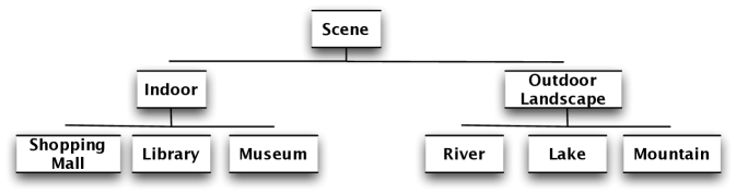
(a) Taxonomy of the 6-scene dataset

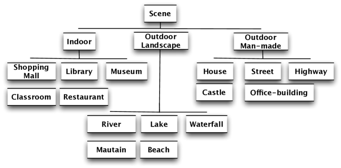
(b) Taxonomy of the 15-scene dataset

Figure 1: The hierarchy structures of two selected subsets of the SUN dataset [34] used in our experiments for hierarchical image classification.

Hierarchical classification with taxonomies

In many applications such as object categorization and document classification [35], classes of objects are organized in taxonomies or hierarchies. For example, the ImageNet dataset has organized all the classes according to the tree structures of WordNet [36]. This problem is a classification example that the output space has interdependent structures. An example tree structure (taxonomy) of image categories is shown in Figure 1.

Now we consider the taxonomy to be a tree, with a partial order $\prec$, which indicates if a class is a predecessor of another class. We override the indicator function, which indicates if $z$ is a predecessor of $y$ in a label tree:

$$\mathbbm{1}(y,z)=\begin{cases}1&y\prec z\text{ or }y=z,\\ 0&\mbox{ otherwise. }\end{cases}$$ (19)

The label coding vector has the same format as in the standard multi-class classification case:

$$\Gamma(y)=[\mathbbm{1}(y,1),\cdots,\mathbbm{1}(y,k)]^{\!\top}\in\{0,1\}^{k}.$$ (20)

Thus $\Gamma(y)^{\!\top}\Gamma(y^{\prime})$ counts the number of common predecessors, while in the case of standard multi-class classification, $\Gamma(y)^{\!\top}\Gamma(y^{\prime})=0$ for $y\neq y^{\prime}$.

Figure 2 shows an example of the label coding vector for a given label hierarchy. In this case, for example, for class 3, $\Gamma(3)=[0,0,1,0,0,0,1,0,1]^{\!\top}$. The joint mapping function is ${\Psi}({\boldsymbol{x}},y)={\Phi}({\boldsymbol{x}})\otimes\Gamma(y).$ The tree loss function ${\Delta}(y,y^{\prime})$ is the height of the first common ancestor of the arguments $y,y^{\prime}$ in the tree. By re-defining $\Gamma(y)$ and ${\Delta}(y,y^{\prime})$, classification with taxonomies can be immediately implemented using the standard multi-class classification shown in the last subsection.

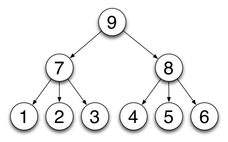
Figure 2: Classification with taxonomies (tree loss), corresponding to the first example in Figure 1.

Here we also consider an alternative approach. In [37], the authors show that one can train a multi-class boosting classifier by projecting data to a label-specific space and then learn a single model parameter ${\boldsymbol{w}}$. The main advantage might be that the optimization of ${\boldsymbol{w}}$ is simplified. Similar to [37] we define label-augmented data as ${\boldsymbol{x}}_{y}^{\prime}={\boldsymbol{x}}\otimes\Gamma(y)$. The max-margin classification can be written as

$$\min_{{{\boldsymbol{w}}\geq 0,\boldsymbol{\xi}\geq 0}}\;\; {\mathbf{1}}^{\!\top}{\boldsymbol{w}}+{\tfrac{C}{m}}{\mathbf{1}}^{\!\top}{\boldsymbol{\xi}}$$

$${{\rm s.t.}\!:}\;\; {\boldsymbol{w}}^{\!\top}\biggl{[}{\Phi}({\boldsymbol{x}}^{\prime}_{i,y_{i}})-{\Phi}({\boldsymbol{x}}^{\prime}_{i,y})\biggr{]}\geq{\Delta}(y_{i},y)-\xi_{i},$$

$$\quad\quad\quad\forall i=1,\cdots,m;\text{ and }\forall y.$$

Compared with the first approach, now the model ${\boldsymbol{w}}\in\mathbb{R}^{n}$, which is independent of the number of classes.

Optimization of the Pascal image overlap criterion

Object detection/localization has used the image area overlap as the loss function [3, 1, 2], e.g, in the Pascal object detection challenge:

$${\Delta}({\boldsymbol{y}},{\boldsymbol{y}}^{\prime})=1-\frac{{\rm area}({\boldsymbol{y}}\cap{\boldsymbol{y}}^{\prime})}{{\rm area}({\boldsymbol{y}}\cup{\boldsymbol{y}}^{\prime})},$$ (21)

with ${\boldsymbol{y}},{\boldsymbol{y}}^{\prime}$ being the bounding box coordinates. ${\boldsymbol{y}}\cap{\boldsymbol{y}}^{\prime}$ and ${\boldsymbol{y}}\cup{\boldsymbol{y}}^{\prime}$ are the box intersection and union. Let ${\boldsymbol{x}}_{\boldsymbol{y}}$ denote an image patch defined by a bounding box ${\boldsymbol{y}}$ on the image ${\boldsymbol{x}}$. To apply StructBoost, we define ${\Psi}({\boldsymbol{x}},{\boldsymbol{y}})={\Phi}({\boldsymbol{x}}_{\boldsymbol{y}})$. ${\Phi}(\cdot)$ is defined in (13). Weak learners such as classifiers or regressors $\varphi(\cdot)$ are trained on the image features extracted from image patches. For example, we can extract histograms of oriented gradients (HOG) from the image patch ${\boldsymbol{x}}_{\boldsymbol{y}}$ and train a decision stump with the extracted HOG features by solving the $\operatorname*{argmax\,}$ in (2.1).

Note that in this case, solving (12), which is to find the most violated constraint in the training step as well as the inference for prediction (2), is in general difficult. In [3], a branch-and-bound search has been employed to find the global optimum. Following the simple sampling strategy in [1], we simplify this problem by evaluating a certain number of sampled image patches to find the most violated constraint. It is also the case for prediction.

CRF parameter learning

CRF has found successful applications in many vision problems such as pixel labelling, stereo matching and image segmentation. Previous work often uses tedious cross-validation for setting the CRF parameters. This approach is only feasible for a small number of parameters. Recently, SSVM has been introduced to learn the parameters [16]. We demonstrate here how to employ the proposed StructBoost for CRF parameter learning in the image segmentation task. We demonstrate the effectiveness of our approach on the Graz-02 image segmentation dataset.

To speed up computation, super-pixels rather than pixels have been widely adopted in image segmentation. We define ${\boldsymbol{x}}$ as an image and ${\boldsymbol{y}}$ as the segmentation labels of all super-pixels in the image. We consider the energy $E$ of an image ${\boldsymbol{x}}$ and segmentation labels ${\boldsymbol{y}}$ over the nodes $\cal N$ and edges $\cal S$, which takes the following form:

$$E({\boldsymbol{x}},{\boldsymbol{y}};{\boldsymbol{w}}) =\sum_{p\in{\cal N}}{\boldsymbol{w}}^{(1){\!\top}}{\Phi}^{(1)}\left(\mathbf{U}(y^{p},{\boldsymbol{x}})\right)$$

$$+\sum_{(p,q)\in{\cal S}}{\boldsymbol{w}}^{(2){\!\top}}{\Phi}^{(2)}\left(\mathbf{V}(y^{p},y^{q},{\boldsymbol{x}})\right).$$ (22)

Recall that $\mathbbm{1}(\cdot,\cdot)$ is the indicator function defined in (16). $p$ and $q$ are the super-pixel indices; $y^{p},y^{q}$ are the labels of the super-pixel $p,q$. $\mathbf{U}$ is a set of unary potential functions: $\mathbf{U}=[\,U_{1},U_{2},\dots]^{\!\top}$. $\mathbf{V}$ is a set of pairwise potential functions: $\mathbf{V}=[\,V_{1},V_{2},\dots]^{\!\top}$. When we learn the CRF parameters, the learning algorithm sees only $\mathbf{U}$ and $\mathbf{V}$. In other words $\mathbf{U}$ and $\mathbf{V}$ play the role as the input features. Details on how to construct $\mathbf{U}$ and $\mathbf{V}$ are described in the experiment part. ${\boldsymbol{w}}^{(1)}$ and ${\boldsymbol{w}}^{(2)}$ are the CRF potential weighting parameters that we aim to learn. ${\Phi}^{(1)}(\cdot)$ and ${\Phi}^{(2)}(\cdot)$ are two sets of weak learners (e.g., decision stumps) for the unary part and pairwise part respectively: ${\Phi}^{(1)}(\cdot)=[\,\varphi_{1}^{(1)}(\cdot),\varphi_{2}^{(1)}(\cdot),\dots]^{\!\top}$, ${\Phi}^{(2)}(\cdot)=[\,\varphi_{1}^{(2)}(\cdot),\varphi_{2}^{(2)}(\cdot),\dots]^{\!\top}$.

To predict the segmentation labels ${\boldsymbol{y}}^{\star}$ of an unknown image ${\boldsymbol{x}}$ is to solve the energy minimization problem:

$${\boldsymbol{y}}^{\star}=\operatorname*{argmin\,}_{{\boldsymbol{y}}}E({\boldsymbol{x}},{\boldsymbol{y}};{\boldsymbol{w}}),$$ (23)

which can be solved efficiently by using graph cuts [16, 38].

Consider a segmentation problem with two classes (background versus foreground). It is desirable to keep the submodular property of the energy function in (3). Otherwise graph cuts cannot be directly applied to achieve globally optimal labelling. Let us examine the pairwise energy term:

$$\theta_{(p,q)}(y^{p},y^{q})={\boldsymbol{w}}^{(2){\!\top}}{\Phi}^{(2)}\left(\mathbf{V}(y^{p},y^{q},{\boldsymbol{x}})\right),$$

and a super-pixel label $y\in\{0,1\}$. It is well known that, if the following is satisfied for any pair $(p,q)\in{\cal S}$, the energy function in (3) is submodular:

$$\theta_{(p,q)}(0,0)+\theta_{(p,q)}(1,1)\leq\theta_{(p,q)}(0,1)+\theta_{(p,q)}(1,0).$$ (24)

We want to keep the above property.

First, for a weak learner $\varphi^{(2)}(\cdot)$, we enforce it to output $0$ when two labels are identical. This can always be achieved by multiplying $(1-\mathbbm{1}(y^{p},y^{q}))$ to a conventional weak learner. Now we have $\theta_{(p,q)}(0,0)$ $=$ $\theta_{(p,q)}(1,1)=0$.

Given that the nonnegative-ness of ${\boldsymbol{w}}$ is enforced in our model, now a sufficient condition is that the output of a weak learner $\varphi^{(2)}(\cdot)$ is always nonnegative, which can always be achieved. We can always use a weak learner $\varphi^{(2)}(\cdot)$ which takes a nonnegative output, e.g., a discrete decision stump or tree with outputs in $\{0,1\}$.

By applying weak learners on $\mathbf{U}$ and $\mathbf{V}$, our method introduces nonlinearity for the parameter learning, which is different from most linear CRF learning methods such as [16]. Until recently, Berteli et al. presented an image segmentation approach that uses nonlinear kernels for the unary energy term in the CRF model [14]. In our model, nonlinearity is introduced by applying weak learners on the potential functions’ outputs. This is the same as the fact that an SVM introduces nonlinearity via the so-called kernel trick and boosting learns a nonlinear model with nonlinear weak learners. Nowozin et al.  [39] introduced decision tree fields (DTF) to overcome the problem of overly-simplified modeling of pairwise potentials in most CRF models. In DTF, local interactions between multiple variables are determined by means of decision trees. In our StructBoost, if we use decision trees as the weak learners on the pairwise potentials, then StructBoost and DTF share similar characteristics in that both use decision trees for the same purpose. However, the starting points of these two methods as well as the training procedures are entirely different.

To apply StructBoost, the CRF parameter learning problem in a large-margin framework can then be written as:

$$\min_{{{\boldsymbol{w}}\geq 0,\boldsymbol{\xi}\geq 0}}\;\; {\mathbf{1}}^{\!\top}{\boldsymbol{w}}+{\tfrac{C}{m}}{\mathbf{1}}^{\!\top}{\boldsymbol{\xi}}$$ (25a)

$${{\rm s.t.}\!:}\;\; E({\boldsymbol{x}}_{i},{\boldsymbol{y}};{\boldsymbol{w}})-E({\boldsymbol{x}}_{i},{\boldsymbol{y}}_{i};{\boldsymbol{w}})\geq{\Delta}({\boldsymbol{y}}_{i},{\boldsymbol{y}})-\xi_{i},$$

$$\quad\quad\quad\forall i=1,\dots,m;\text{ and }\forall{\boldsymbol{y}}\in{\cal Y}.$$ (25b)

Here $i$ indexes images. Intuitively, the optimization in (25) is to encourage the energy of the ground truth label $E({\boldsymbol{x}}_{i},{\boldsymbol{y}}_{i})$ to be lower than any other incorrect labels $E({\boldsymbol{x}}_{i},{\boldsymbol{y}})$ by at least a margin ${\Delta}({\boldsymbol{y}}_{i},{\boldsymbol{y}})$, $\forall{\boldsymbol{y}}$. We simply define ${\Delta}({\boldsymbol{y}}_{i},{\boldsymbol{y}})$ using the Hamming loss, which is the sum of the differences between the ground truth label ${\boldsymbol{y}}_{i}$ and the label ${\boldsymbol{y}}$ over all super-pixels in an image:

$${\Delta}({\boldsymbol{y}}_{i},{\boldsymbol{y}})=\sum_{p}(1-\mathbbm{1}(y_{i}^{p},y^{p})).$$ (26)

We show the problem (25) is a special case of the general formulation of StructBoost (35) by defining

$${\boldsymbol{w}}=-{\boldsymbol{w}}^{(1)}\odot{\boldsymbol{w}}^{(2)},$$

and,

$${\Psi}({\boldsymbol{x}},{\boldsymbol{y}}) =\sum_{p\in\cal N}{\Phi}^{(1)}\left(\mathbf{U}(y^{p},{\boldsymbol{x}})\right)\odot\sum_{(p,q)\in\cal S}{\Phi}^{(2)}\left(\mathbf{V}(y^{p},y^{q},{\boldsymbol{x}})\right).$$

Recall that $\odot$ stacks two vectors. With this definition, we have the relation:

$${\boldsymbol{w}}^{\!\top}{\Psi}({\boldsymbol{x}},{\boldsymbol{y}})=-E({\boldsymbol{x}},{\boldsymbol{y}};{\boldsymbol{w}}).$$

The minus sign here is to inverse the order of subtraction in (35b). At each column generation iteration (Algorithm 1), two new weak learners $\varphi^{(1)}(\cdot)$ and $\varphi^{(2)}(\cdot)$ are added to the unary weak learner set and the pairwise weak learner set, respectively by solving the $\operatorname*{argmax\,}$ problem defined in (2.1), which can be written as:

$$\varphi^{(1)\star}(\cdot)= \operatorname*{argmax\,}_{\varphi(\cdot)}\sum_{i,{\boldsymbol{y}}}\mu_{(i,{\boldsymbol{y}})}\sum_{p\in\cal N}\Bigl{[}\varphi^{(1)}\left(\mathbf{U}(y^{p},{\boldsymbol{x}}_{i})\right)$$

$$-\varphi^{(1)}\left(\mathbf{U}(y^{p}_{i},{\boldsymbol{x}}_{i}\right)\Bigr{]};$$ (27)

$$\varphi^{(2)\star}(\cdot)= \operatorname*{argmax\,}_{\varphi(\cdot)}\sum_{i,{\boldsymbol{y}}}\mu_{(i,{\boldsymbol{y}})}\sum_{(p,q)\in\cal S}\Bigl{[}\varphi^{(2)}\left(\mathbf{V}(y^{p},y^{q},{\boldsymbol{x}}_{i})\right)$$

$$-\varphi^{(2)}\left(\mathbf{V}(y_{i}^{p},y_{i}^{q},{\boldsymbol{x}}_{i})\right)\Bigr{]}.$$ (28)

The maximization problem to find the most violated constraint in (12) is to solve the inference:

$${\boldsymbol{y}}^{\prime}_{i}=\operatorname*{argmin\,}_{{\boldsymbol{y}}}E({\boldsymbol{x}}_{i},{\boldsymbol{y}})-{\Delta}({\boldsymbol{y}}_{i},{\boldsymbol{y}}),$$ (29)

which is similar to the label prediction inference in (23), and the only difference is that the labeling loss term: ${\Delta}({\boldsymbol{y}}_{i},{\boldsymbol{y}})$ is involved in (29). Recall that we use the Hamming loss ${\Delta}({\boldsymbol{y}}_{i},{\boldsymbol{y}})$ as defined in (26), the term ${\Delta}({\boldsymbol{y}}_{i},{\boldsymbol{y}})$ can be absorbed into the unary term of the energy function defined in (3) (such as in [16]). The inference in (29) can be written as:

$${\boldsymbol{y}}_{i}^{\prime}=\operatorname*{argmin\,}_{{\boldsymbol{y}}} \sum_{p\in\cal N}\biggr{[}{\boldsymbol{w}}^{(1){\!\top}}{\Phi}^{(1)}\left(\mathbf{U}(y^{p},{\boldsymbol{x}}_{i})\right)-(1-\mathbbm{1}(y_{i}^{p},y^{p}))\biggr{]}$$

$$+\sum_{(p,q)\in\cal S}{\boldsymbol{w}}^{(2){\!\top}}{\Phi}^{(2)}\left(\mathbf{V}(y^{p},y^{q},{\boldsymbol{x}}_{i})\right).$$ (30)

The above minimization (3) can also be solved efficiently by using graph cuts.

4 Experiments

To evaluate our method, we run various experiments on applications including AUC maximization (ordinal regression), multi-class image classification, hierarchical image classification, visual tracking and image segmentation. We mainly compare with the most relevant method: Structured SVM (SSVM) and some other conventional methods (e.g., SVM, AdaBoost). If not otherwise specified, the cutting-plane stopping criteria ($\epsilon_{\rm cp}$) in our method is set to $0.01$.

TABLE I: AUC maximization. We compare the performance of $m$-slack and $1$-slack  formulations. “$-$” means that the method is not able to converge within a memory and time limit. We can see that $1$-slack can achieve similar AUC results on training and testing data as $m$-slack while $1$-slack is significantly faster than $m$-slack.

dataset	method	time (sec)	AUC training	AUC test
wine	$m$-slack	13$\pm$1	1.000$\pm$0.000	0.994$\pm$0.005
	$1$-slack	3$\pm$1	1.000$\pm$0.000	0.994$\pm$0.006
glass	$m$-slack	20$\pm$1	0.967$\pm$0.011	0.849$\pm$0.028
	$1$-slack	6$\pm$1	0.955$\pm$0.030	0.844$\pm$0.039
svmguide2	$m$-slack	332$\pm$6	0.988$\pm$0.003	0.905$\pm$0.036
	$1$-slack	106$\pm$8	0.988$\pm$0.003	0.905$\pm$0.036
svmguide4	$m$-slack	564$\pm$79	1.000$\pm$0.000	0.982$\pm$0.005
	$1$-slack	106$\pm$13	1.000$\pm$0.000	0.982$\pm$0.005
vowel	$m$-slack	4051$\pm$116	0.999$\pm$0.001	0.968$\pm$0.013
	$1$-slack	952$\pm$139	0.999$\pm$0.001	0.967$\pm$0.013
dna	$m$-slack	$-$	$-$	$-$
	$1$-slack	1598$\pm$643	0.998$\pm$0.000	0.992$\pm$0.003
segment	$m$-slack	$-$	$-$	$-$
	$1$-slack	475$\pm$42	1.000$\pm$0.000	0.999$\pm$0.001
satimage	$m$-slack	$-$	$-$	$-$
	$1$-slack	37769$\pm$6331	0.999$\pm$0.000	0.997$\pm$0.002

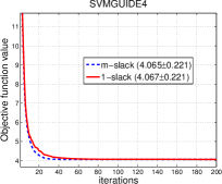
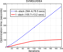
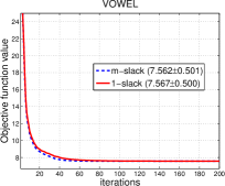
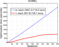
Figure 3: AUC optimization on two UCI datasets. The objective values and optimization time are shown in the figure by varying boosting (or column generation) iterations. It shows that $1$-slack achieves similar objective values as $m$-slack but needs less running time.

AUC optimization

In this experiment, we compare efficiency of the $1$-slack (solving (38)) and $m$-slack (solving (35) or its dual) formulations of our method StructBoost. The details for AUC optimization are described in Section 3. We run the experiments on a few UCI multi-class datasets. To create imbalanced data, we use one class of the multi-class UCI datasets as positive data and the rest as negative data. The boosting (column generation) iteration is set to 200; the cutting-plane stopping criterion ($\epsilon_{\rm cp}$) is set to 0.001. Decision stumps are used as weak learners (${\Phi}(\cdot)$ in (14)). For each data set, we randomly sample 50% for training, 25% for validation and the rest for testing. The regularization parameter $C$ is chosen from 6 candidates ranging from $10$ to $10^{3}$. Experiments are repeated 5 times on each dataset and the mean and standard deviation are reported. Table I reports the results. We can see that the $1$-slack  formulation of StructBoost achieves similar AUC performance as the $m$-slack formulation, while being much faster than $m$-slack. The values of objective function and optimization time are shown in Figure 3 by varying column generation iterations. Again, it shows that $1$-slack achieves similar objective values as $m$-slack with less running time.

Note that RankBoost may also be applied to this problem [40]. RankBoost has been designed for solving ranking problems.

TABLE II: Multi-class classification test errors (%) on several UCI and MNIST datasets. StructBoost-stump and StructBoost-per denote our StructBoost using decision stumps and perceptrons as weak learners, respectively. StructBoost outperforms SSVM in most cases and achieves competitive performance compared with other multi-class classifiers.

	glass	svmguide2	svmguide4	vowel	dna	segment	satimage	usps	pendigits	mnist
StructBoost-stump	35.8 $\pm$ 6.2	21.0 $\pm$ 3.9	20.1 $\pm$ 2.9	17.5 $\pm$ 2.2	6.2 $\pm$ 0.7	2.9 $\pm$ 0.7	12.1 $\pm$ 0.7	6.9 $\pm$ 0.6	3.9 $\pm$ 0.4	12.5 $\pm$ 0.4
StructBoost-per	37.3 $\pm$ 6.2	22.7 $\pm$ 4.8	53.4 $\pm$ 6.1	6.8 $\pm$ 1.8	6.6 $\pm$ 0.6	3.8 $\pm$ 0.7	11.4 $\pm$ 1.1	4.1 $\pm$ 0.6	1.8 $\pm$ 0.3	6.5 $\pm$ 0.6
Ada.ECC	32.7 $\pm$ 4.9	23.3 $\pm$ 4.0	19.1 $\pm$ 2.3	20.6 $\pm$ 1.5	7.6 $\pm$ 1.2	2.9 $\pm$ 0.8	12.8 $\pm$ 0.7	8.4 $\pm$ 0.7	8.4 $\pm$ 0.7	15.8 $\pm$ 0.3
Ada.MH	32.3 $\pm$ 5.0	21.9 $\pm$ 4.5	19.3 $\pm$ 3.0	18.8 $\pm$ 2.1	7.1 $\pm$ 0.6	3.7 $\pm$ 0.7	12.7 $\pm$ 0.9	7.4 $\pm$ 0.5	7.4 $\pm$ 0.5	13.4 $\pm$ 0.4
SSVM	38.8 $\pm$ 8.7	21.9 $\pm$ 5.9	45.7 $\pm$ 3.9	25.6 $\pm$ 2.5	6.9 $\pm$ 0.9	5.3 $\pm$ 1.0	14.9 $\pm$ 0.1	5.8 $\pm$ 0.3	5.2 $\pm$ 0.3	9.6 $\pm$ 0.2
1-vs-all SVM	40.8 $\pm$ 7.0	17.7 $\pm$ 3.5	47.0 $\pm$ 3.2	54.4 $\pm$ 2.2	6.3 $\pm$ 0.5	7.7 $\pm$ 0.8	17.5 $\pm$ 0.4	5.4 $\pm$ 0.5	8.1 $\pm$ 0.5	9.2 $\pm$ 0.2

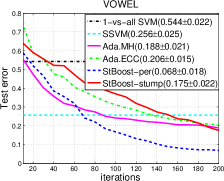
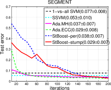
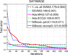
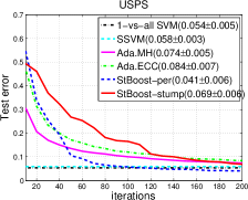
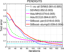
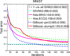
Figure 4: Test performance versus the number of boosting iterations of multi-class classification. StBoost-stump and StBoost-per denote our StructBoost using decision stumps and perceptrons as weak learners, respectively. The results of SSVM and SVM are shown as straight lines in the plots. The values shown in the legend are the error rates of the final iteration for each method. Our methods perform better than SSVM in most cases.

Multi-class classification

Multi-class classification is a special case of structured learning. Details are described in Section 3. We carry out experiments on some UCI multi-class datasets and MNIST. We compare with Structured SVM (SSVM), conventional multi-class boosting methods (namely AdaBoost.ECC and AdaBoost.MH), and the one-vs-all SVM method. For each dataset, we randomly select 50% data for training, 25% data for validation and the rest for testing. The maximum number of boosting iterations is set to 200; the regularization parameter $C$ is chosen from 6 candidates whose values range from 10 to $1000$. The experiments are repeated 5 times for each dataset.

To demonstrate the flexibility of our method, we use decision stumps and linear perceptron functions as weak learners (${\Phi}(\cdot)$ in (17)). The perceptron weak learner can be written as:

$$\varphi({\boldsymbol{x}})=\mathrm{sign}({\boldsymbol{v}}^{\!\top}{\boldsymbol{x}}+b).$$ (31)

We use a smooth sigmoid function to replace the step function so that gradient descent optimization can be applied. We solve the $\operatorname*{argmax\,}$ problem in (18) by using the Quasi-Newton LBFGS [41] solver. We found that decision stumps often provide a good initialization for LBFGS learning of the perceptron. Compared with decision stumps, using the perceptron weak learner usually needs fewer boosting iterations to converge. Table II reports the error rates. Figure 4 shows test performance versus the number of boosting (column generation) iterations. The results demonstrate that our method outperforms SSVM, and achieves competitive performance compared with other conventional multi-class methods.

StructBoost performs better than SSVM on most datasets. This might be due to the introduction of non-linearity in StructBoost. Results also show that using the perceptron weak learner often achieves better performance than using decision stumps on those large datasets.

TABLE III: Hierarchical classification. Results of the tree loss and the 1/0 loss (classification error rate) on subsets of the SUN dataset. StructBoost-tree uses the hierarchy class formulation with the tree loss, and StructBoost-flat uses the standard multi-class formulation. StructBoost-tree that minimizes the tree loss performs best.

datasets		StructBoost-tree	StructBoost-flat	Ada.ECC-SVM	Ada.ECC	Ada.MH
6 scenes	1/0 loss	0.322 $\pm$ 0.018	0.343 $\pm$ 0.028	0.350 $\pm$ 0.013	0.327 $\pm$ 0.002	0.315 $\pm$ 0.015
	tree loss	0.337 $\pm$ 0.014	0.380 $\pm$ 0.027	0.377 $\pm$ 0.018	0.352 $\pm$ 0.023	0.346 $\pm$ 0.018
15 scenes	1/0 loss	0.394 $\pm$ 0.005	0.396 $\pm$ 0.013	0.414 $\pm$ 0.012	0.444 $\pm$ 0.012	0.418 $\pm$ 0.010
	tree loss	0.504 $\pm$ 0.007	0.536 $\pm$ 0.009	0.565 $\pm$ 0.019	0.584 $\pm$ 0.017	0.551 $\pm$ 0.013

4.1 Hierarchical multi-class classification

The details of hierarchical multi-class are described in Section 3. We have constructed two hierarchical image datasets from the SUN dataset [34] which contains 6 classes and 15 classes of scenes. The hierarchical tree structures of these two datasets are shown in the Figure 1. For each scene class, we use the first 200 images from the original SUN dataset. There are 1200 images in the first dataset and 3000 images in the second dataset. We have used the HOG features as described in [34]. For each dataset, 50% examples are randomly selected for training and the rest for testing. We run 5 times for each dataset. The regularization parameter is chosen from 6 candidates ranging from 1 to $10^{3}$.

We use linear SVM as weak classifiers in our method. The linear SVM weak classifier has the same form as (31). At each boosting iteration, we solve the $\operatorname*{argmax\,}$ problem by training a linear SVM model. The regularization parameter $C$ in SVM is set to a large value ($10^{8}$/#examples). To alleviate the overfitting problem of using linear SVM as weak learners, we set 10% of the smallest non-zero dual solutions $\mu_{(i,{\boldsymbol{y}})}$ to zero.

We compare StructBoost using the hierarchical multi-class formulation (StructBoost-tree) and the standard multi-class formulation (StructBoost-flat). We run some other multi-class methods for further comparison: Ada.ECC, Ada.MH with decision stumps. We also run Ada.ECC using linear SVM as weak classifiers (labelled as Ada.ECC-SVM).

When using SVM as weak learners, the number of boosting iterations is set to 200, and for decision stump, it is set to 500. Table III shows the tree loss and the 1/0 loss (classification error rate). We observe that StructBoost-tree has the lowest tree loss among all compared methods, and it also improves its counterpart, StructBoost-flat, in terms of both classification error rates and the tree loss. Our StructBoost-tree makes use of the class hierarchy information and directly optimizes the tree loss. That might be the reason why StructBoost-tree achieves best performance.

Visual tracking

A visual tracking method, termed Struck [1], was introduced based on SSVM. The core idea is to train a tracker by optimizing the Pascal image overlap score using SSVM. Here we apply StructBoost to visual tracking, following the similar setting as in Struck [1]. More details can be found in Section 3.

Our experiment follows the on-line tracking setting. Here we use the first 3 labeled frames for initialization and training of our StructBoost tracker. Then the tracker is updated by re-training the model during the course of tracking. Specifically, in the $i$-th frame (represented by ${\boldsymbol{x}}_{i}$), we first perform a prediction step (solving (2)) to output the detection box (${\boldsymbol{y}}_{i}$), then collect training data for tracker update. For solving the prediction inference in (2), we simply sample about 2000 bounding boxes around the prediction box of the last frame (represented by ${\boldsymbol{y}}_{i-1}$), and search for the most confident bounding box over all sampled boxes as the prediction. After the prediction, we collect training data by sampling about 200 bounding boxes around the current prediction ${\boldsymbol{y}}_{i}$. We use the training data in recent 60 frames to re-train the tracker for every 2 frames. Solving (12) for finding the most violated constraint is similar to the prediction inference.

For StructBoost, decision stumps are used as the weak classifiers; the number of boosting iterations is set to 300; the regularization parameter $C$ is selected from $10^{0.5}$ to $10^{2}$. We use the down-scaled gray-scale raw pixels and HOG [42] as image features.

For comparison, we also run a simple binary AdaBoost tracker using the same setting as our StructBoost tracker. The number of weak classifiers for AdaBoost is set to 500. When training the AdaBoost tracker, we collect positive boxes that significantly overlap (overlap score above $0.8$) with the prediction box of the current frame, and negative boxes with small overlap scores (lower or equal to $0.3$).

We also compare with a few state-of-the-art tracking methods, including Struck [1] (with a buffer size of 50), multi-instance tracking (MIL) [43], fragment tracking (Frag) [44], online AdaBoost tracking (OAB) [45], and visual tracking decomposition (VTD) [46]. Two different settings are used for OAB: one positive example per frame (OAB₁) and five positive examples per frame (OAB₅) for training. The test video sequences: ”coke, tiger1, tiger2, david, girl and sylv” were used in [1]; “shaking, singer” are from [46] and the rest are from [47].

Table IV reports the Pascal overlap scores of compared methods. Our StructBoost tracker performs best on most sequences. Compared with the simple binary AdaBoost tracker, StructBoost that optimizes the pascal overlap criterion perform significantly better. Note that here Struck uses Haar features. When Struck uses a Gaussian kernel defined on raw pixels, the performance is slightly different [1], and ours still outperforms Struck in most cases. This might be due to the fact that StructBoost selects relevant features (300 features selected here), while SSVM of Struck [1] uses all the image patch information which may contain noises.

The center location errors (in pixels) of compared methods are shown in Table V. We can see that optimizing the overlap score also helps to minimize the center location errors. Our method also achieves the best performance.

Figure 5 plots the Pascal overlap scores and central location errors frame by frame on several video sequences. Some tracking examples are shown in Figure 6.

TABLE IV: Average bounding box overlap scores on benchmark videos. Struck₅₀ [1] is structured SVM tracking with a buffer size of 50. Our StructBoost performs the best in most cases. Struck performs the second best, which confirms the usefulness of structured output learning.

	StructBoost	AdaBoost	Struck50	Frag	MIL	OAB1	OAB5	VTD
coke	0.79 $\pm$ 0.17	0.47 $\pm$ 0.19	0.55 $\pm$ 0.18	0.07 $\pm$ 0.21	0.36 $\pm$ 0.23	0.10 $\pm$ 0.20	0.04 $\pm$ 0.16	0.10 $\pm$ 0.23
tiger1	0.75 $\pm$ 0.17	0.64 $\pm$ 0.16	0.68 $\pm$ 0.21	0.21 $\pm$ 0.30	0.64 $\pm$ 0.18	0.44 $\pm$ 0.23	0.23 $\pm$ 0.24	0.11 $\pm$ 0.24
tiger2	0.74 $\pm$ 0.18	0.46 $\pm$ 0.18	0.59 $\pm$ 0.19	0.16 $\pm$ 0.24	0.63 $\pm$ 0.14	0.35 $\pm$ 0.23	0.18 $\pm$ 0.19	0.19 $\pm$ 0.22
david	0.86 $\pm$ 0.07	0.34 $\pm$ 0.23	0.82 $\pm$ 0.11	0.18 $\pm$ 0.24	0.59 $\pm$ 0.13	0.28 $\pm$ 0.23	0.21 $\pm$ 0.22	0.29 $\pm$ 0.27
girl	0.74 $\pm$ 0.12	0.41 $\pm$ 0.26	0.80 $\pm$ 0.10	0.65 $\pm$ 0.19	0.56 $\pm$ 0.21	0.43 $\pm$ 0.18	0.28 $\pm$ 0.26	0.63 $\pm$ 0.12
sylv	0.66 $\pm$ 0.16	0.52 $\pm$ 0.18	0.69 $\pm$ 0.14	0.61 $\pm$ 0.23	0.66 $\pm$ 0.18	0.47 $\pm$ 0.38	0.05 $\pm$ 0.12	0.58 $\pm$ 0.30
bird	0.79 $\pm$ 0.11	0.67 $\pm$ 0.14	0.60 $\pm$ 0.26	0.34 $\pm$ 0.32	0.58 $\pm$ 0.32	0.57 $\pm$ 0.29	0.59 $\pm$ 0.30	0.11 $\pm$ 0.26
walk	0.74 $\pm$ 0.19	0.56 $\pm$ 0.14	0.59 $\pm$ 0.39	0.09 $\pm$ 0.25	0.51 $\pm$ 0.34	0.54 $\pm$ 0.36	0.49 $\pm$ 0.34	0.08 $\pm$ 0.23
shaking	0.72 $\pm$ 0.13	0.49 $\pm$ 0.22	0.08 $\pm$ 0.19	0.33 $\pm$ 0.28	0.61 $\pm$ 0.26	0.57 $\pm$ 0.28	0.51 $\pm$ 0.21	0.69 $\pm$ 0.14
singer	0.69 $\pm$ 0.10	0.74 $\pm$ 0.10	0.34 $\pm$ 0.37	0.14 $\pm$ 0.30	0.20 $\pm$ 0.34	0.20 $\pm$ 0.33	0.07 $\pm$ 0.18	0.50 $\pm$ 0.20
iceball	0.58 $\pm$ 0.17	0.05 $\pm$ 0.16	0.51 $\pm$ 0.33	0.51 $\pm$ 0.31	0.35 $\pm$ 0.29	0.08 $\pm$ 0.23	0.38 $\pm$ 0.30	0.57 $\pm$ 0.29

TABLE V: Average center errors on benchmark videos. Struck₅₀ [1] is structured SVM tracking with a buffer size of 50. We observe similar results as in Table IV: Our StructBoost outperforms others on most sequences, and Struck is the second best.

	StructBoost	AdaBoost	Struck50	Frag	MIL	OAB1	OAB5	VTD
coke	3.7 $\pm$ 4.5	9.3 $\pm$ 4.2	8.3 $\pm$ 5.6	69.5 $\pm$ 32.0	17.8 $\pm$ 9.6	34.7 $\pm$ 15.5	68.1 $\pm$ 30.3	46.8 $\pm$ 21.8
tiger1	5.4 $\pm$ 4.9	7.8 $\pm$ 4.4	7.8 $\pm$ 9.9	39.6 $\pm$ 25.7	8.4 $\pm$ 5.9	17.8 $\pm$ 16.4	38.9 $\pm$ 31.1	68.8 $\pm$ 36.4
tiger2	5.2 $\pm$ 5.6	12.7 $\pm$ 6.3	8.7 $\pm$ 6.1	38.5 $\pm$ 24.9	7.5 $\pm$ 3.6	20.5 $\pm$ 14.9	38.3 $\pm$ 26.9	38.0 $\pm$ 29.6
david	5.2 $\pm$ 2.8	43.0 $\pm$ 28.2	7.7 $\pm$ 5.7	73.8 $\pm$ 36.7	19.6 $\pm$ 8.2	51.0 $\pm$ 30.9	64.4 $\pm$ 33.5	66.1 $\pm$ 56.3
girl	14.3 $\pm$ 7.8	47.1 $\pm$ 29.5	10.1 $\pm$ 5.5	23.0 $\pm$ 22.5	31.6 $\pm$ 28.2	43.3 $\pm$ 17.8	67.8 $\pm$ 32.5	18.4 $\pm$ 11.4
sylv	9.1 $\pm$ 5.8	14.7 $\pm$ 7.8	8.4 $\pm$ 5.3	12.2 $\pm$ 11.8	9.4 $\pm$ 6.5	32.9 $\pm$ 36.5	76.4 $\pm$ 35.4	21.6 $\pm$ 35.7
bird	6.7 $\pm$ 3.8	12.7 $\pm$ 9.5	17.9 $\pm$ 13.9	50.0 $\pm$ 43.3	49.0 $\pm$ 85.3	47.9 $\pm$ 87.7	48.5 $\pm$ 86.3	143.9 $\pm$ 79.3
walk	8.4 $\pm$ 10.3	13.5 $\pm$ 5.4	33.9 $\pm$ 49.5	102.8 $\pm$ 46.3	35.0 $\pm$ 47.5	35.7 $\pm$ 49.2	38.0 $\pm$ 48.7	100.9 $\pm$ 47.1
shaking	9.5 $\pm$ 5.4	21.6 $\pm$ 12.0	123.9 $\pm$ 54.5	47.2 $\pm$ 40.6	37.8 $\pm$ 75.6	26.9 $\pm$ 49.3	29.1 $\pm$ 48.7	10.5 $\pm$ 6.8
singer	5.8 $\pm$ 2.2	4.8 $\pm$ 2.1	29.5 $\pm$ 23.8	172.8 $\pm$ 95.2	188.3 $\pm$ 120.8	189.9 $\pm$ 115.2	158.5 $\pm$ 68.6	10.1 $\pm$ 7.6
iceball	8.0 $\pm$ 4.1	107.9 $\pm$ 66.4	15.6 $\pm$ 22.1	39.8 $\pm$ 72.9	61.6 $\pm$ 85.6	97.7 $\pm$ 53.5	58.7 $\pm$ 84.0	13.5 $\pm$ 26.0

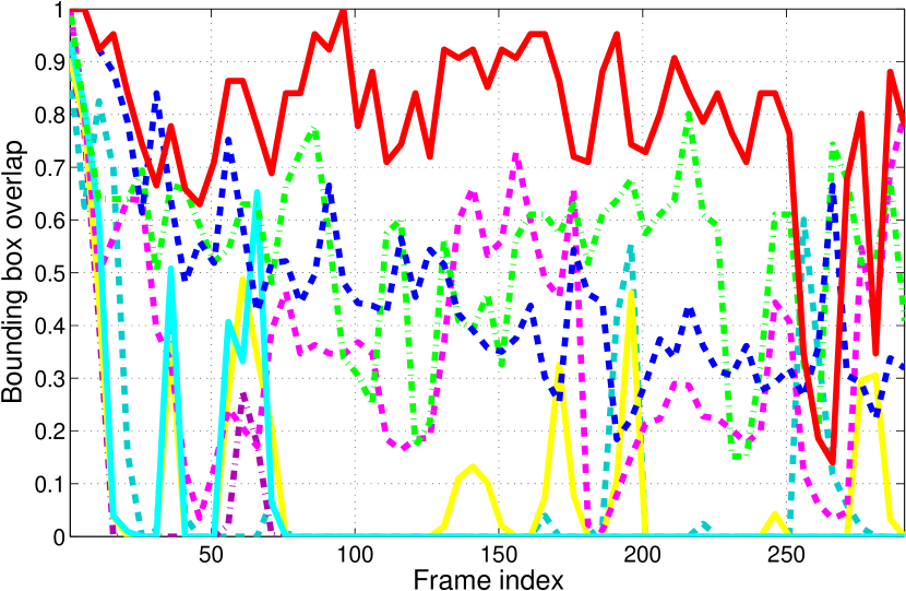
(a) coke

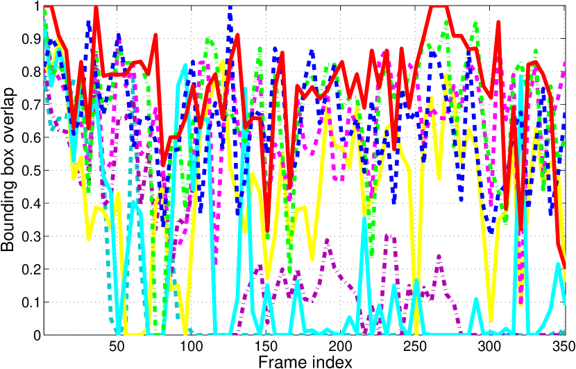
(b) tiger1

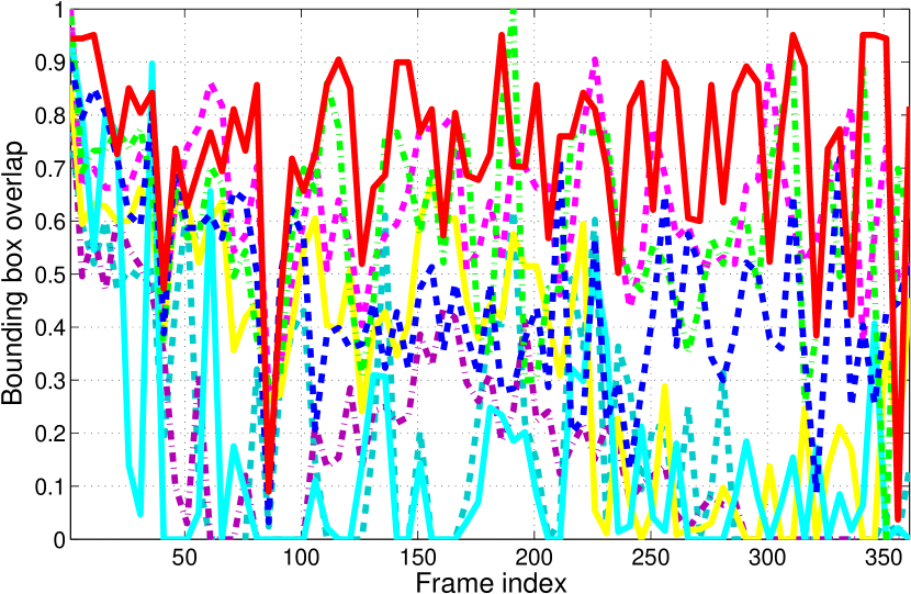
(c) tiger2

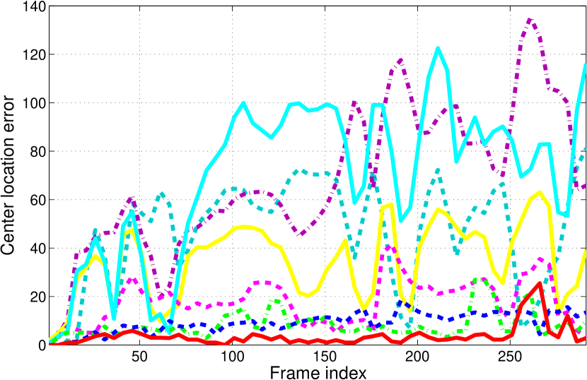
(d) coke

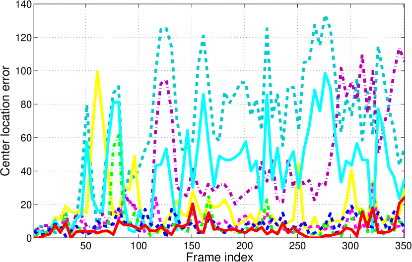
(e) tiger1

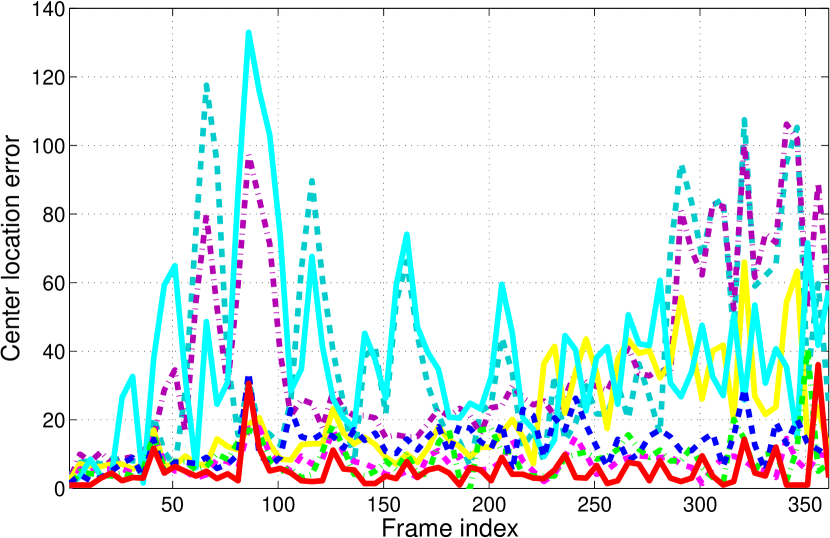
(f) tiger2

Figure 5: Bounding box overlap (first row) and center location error (second row) in frames of several video sequences. Our StructBoost often achieves higher scores of box overlap and lower center location errors compared with other trackers.

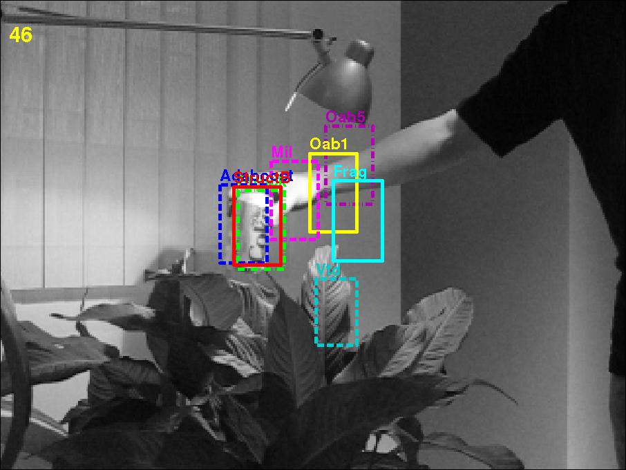
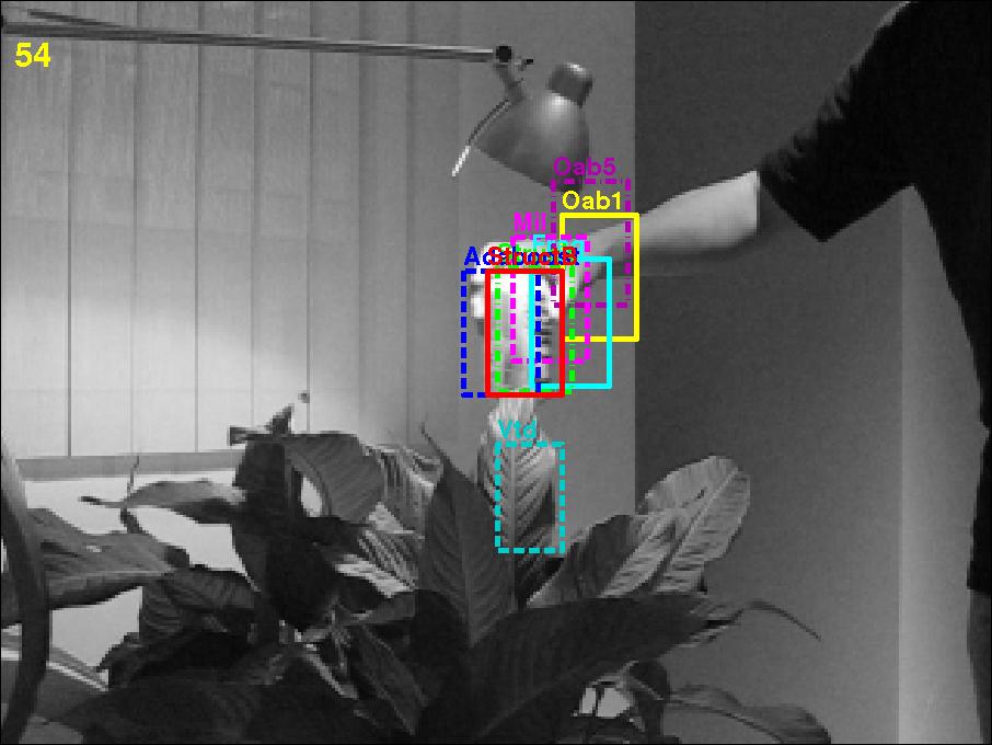
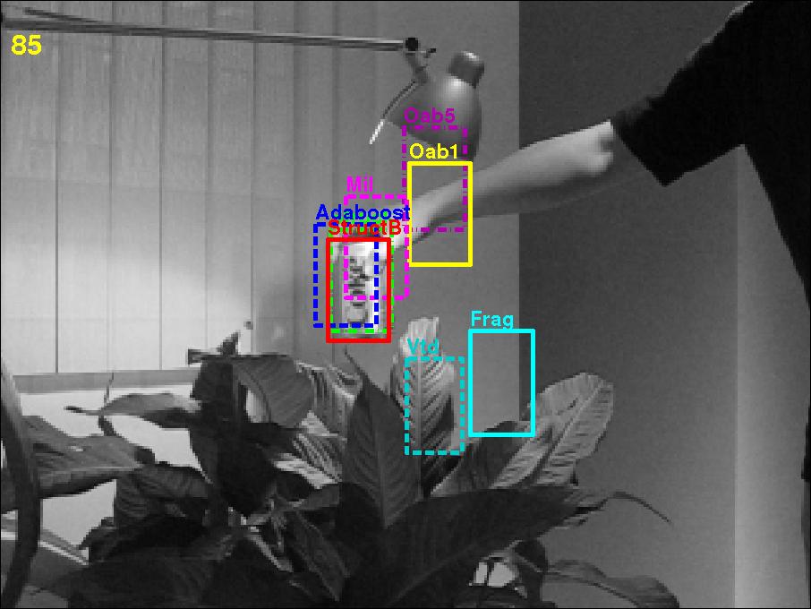
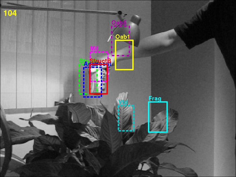
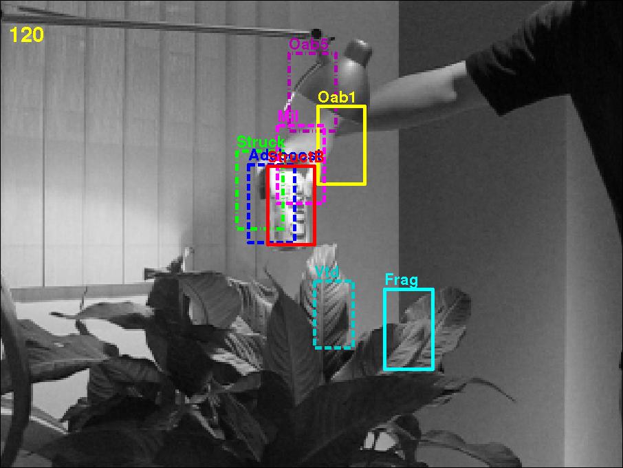
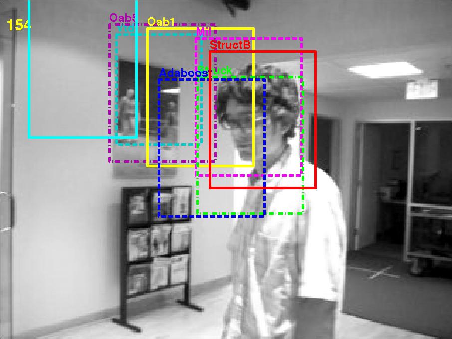
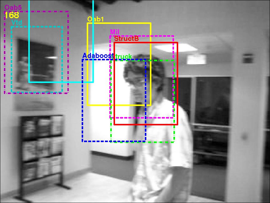
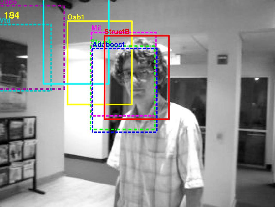
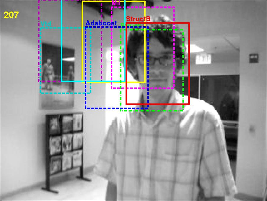
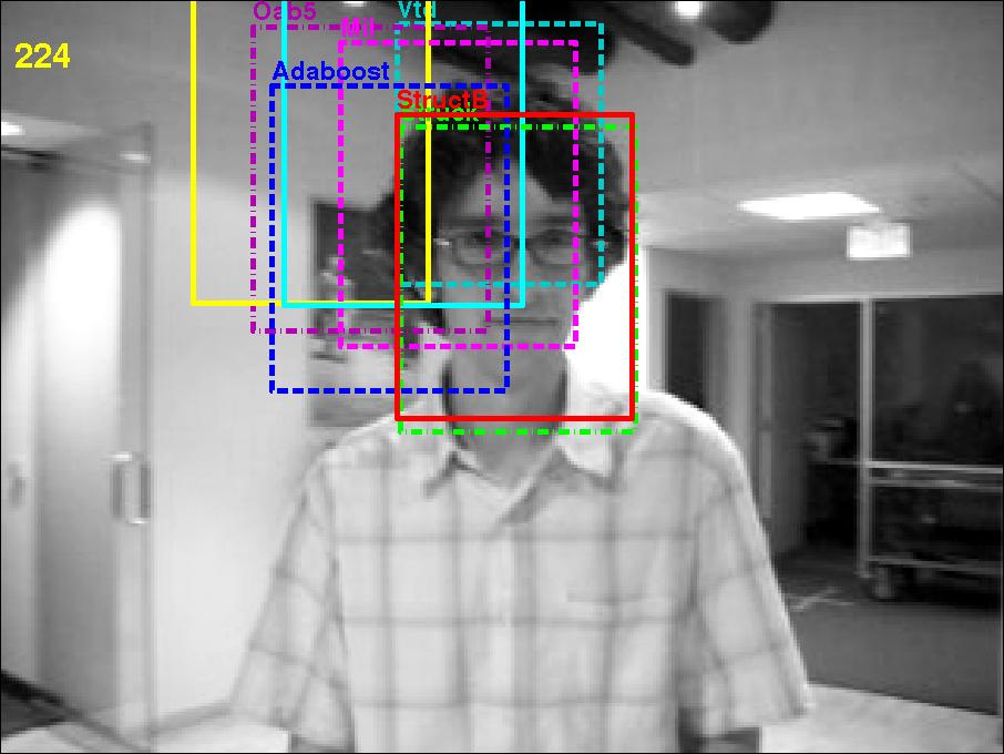
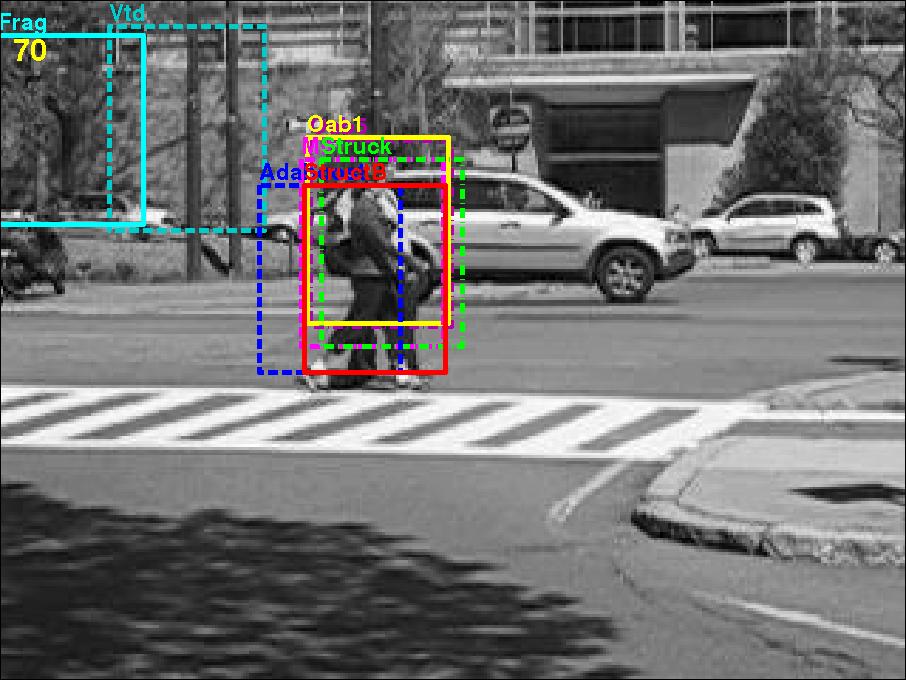
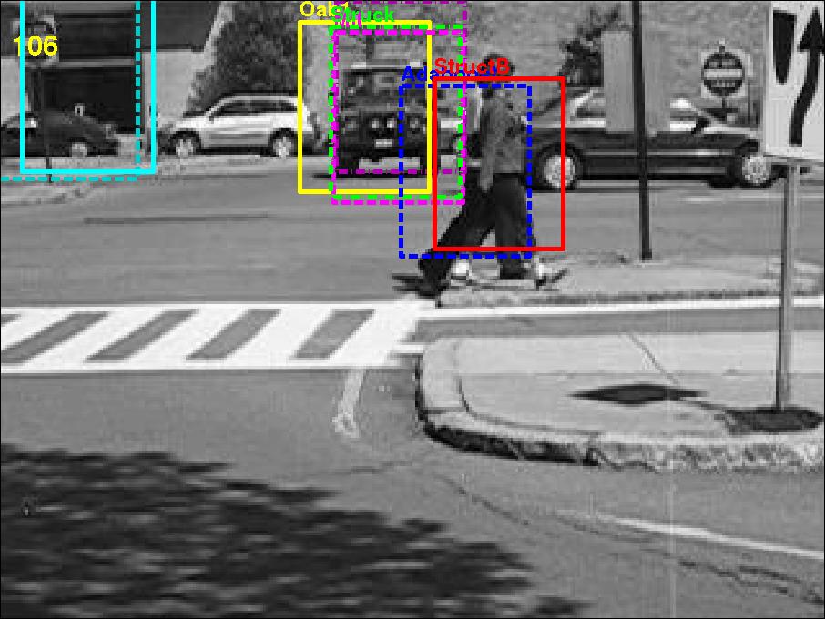
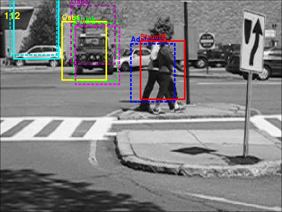
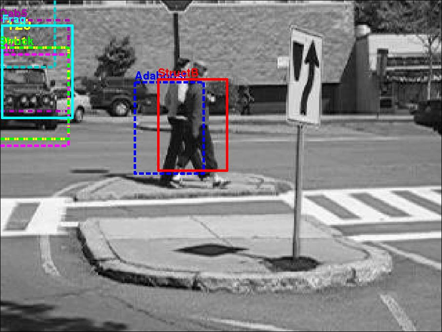
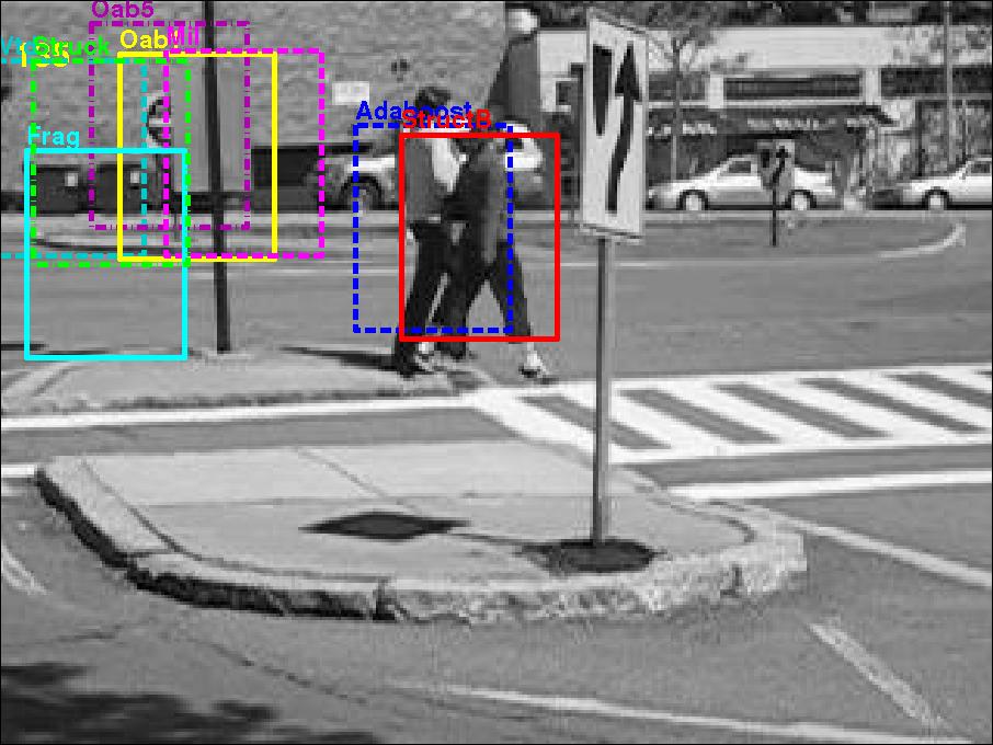
Figure 6: Some tracking examples of several video sequences: “coke”, “david”, and “walk” (best viewed on screen). The output bounding boxes of our StructBoost better overlap against the ground truth than the compared methods.

4.2 CRF parameter learning for image segmentation

We evaluate our method on CRF parameter learning for image segmentation, following the work of [16]. The work of [16] applies SSVM to learn weighting parameters for different potentials (including multiple unary and pairwise potentials). The goal of applying StructBoost here is to learn a non-linear weighting for different potentials. Details are described in Section 3.

We extend the super-pixels based segmentation method [38] with CRF parameter learning. The Graz-02 dataset is used here which contains 3 categories (bike, car and person). Following the setting as other methods [38], the first 300 labeled images in each category are used in the experiment. Images with the odd indices are used for training and the rest for testing. We generate super-pixels using the same setting as [38]. For each super-pixel, we generate 5 types of features: visual word histogram [38], color histograms, GIST [48], LBP and HOG [42]. For constructing the visual word histogram, we follow [38] using a neighborhood size of $2$; the code book size is set to 200. For GIST, LBP and HOG, we extract features from patches centered at the super-pixel with 4 increasing sizes: $4\times 4,8\times 8,12\times 12$ and $16\times 16$. The cell size for LBP and HOG is set to a quarter of the patch size. For GIST, we generate 512 dimensional features for each patch by using 4 scales and the number of orientations is set to 8. In total, we generate 14 groups of features (including features extracted on patches of different sizes). Using these super-pixel features, we construct 14 different unary potentials ($\mathbf{U}=[\,U_{1},\dots,U_{14}\,]^{\!\top}$) from AdaBoost classifiers, which are trained on the foreground and background super-pixels. The number of boosting iterations for AdaBoost is set to $1000$. Specifically, we define $F^{\prime}({\boldsymbol{x}}^{p})$ as the discriminant function of AdaBoost on the features of the $p$-th super-pixel. Then the unary potential function can be written as:

$$U({\boldsymbol{x}},y^{p})=-y^{p}F^{\prime}({\boldsymbol{x}}^{p}).$$ (32)

We also construct 2 pairwise potentials ($\mathbf{V}=[\,V_{1},V_{2}\,]^{\!\top}$): $V_{1}$ is constructed using color difference, and $V_{2}$ using shared boundary length [38] which is able to discourage small isolated segments. Recall that $\mathbbm{1}(\cdot,\cdot)$ is an indicator function defined in (16). $\|{\boldsymbol{x}}^{p}-{\boldsymbol{x}}^{q}\|_{2}$ calculates the $\ell_{2}$ norm of the color difference between two super-pixels in the LUV color-space; $\ell({\boldsymbol{x}}^{p},{\boldsymbol{x}}^{q})$ is the shared boundary length between two super-pixels. Then $V_{1},V_{2}$ can be written as:

$$V_{1}(y^{p},y^{q},{\boldsymbol{x}})= \exp(-\|{\boldsymbol{x}}^{p}-{\boldsymbol{x}}^{q}\|_{2})\bigl{[}1-\mathbbm{1}(y^{p},y^{q})\bigr{]},$$ (33)

$$V_{2}(y^{p},y^{q},{\boldsymbol{x}})= \ell({\boldsymbol{x}}^{p},{\boldsymbol{x}}^{q})\bigl{[}1-\mathbbm{1}(y^{p},y^{q})\bigr{]}.$$ (34)

We apply StructBoost here to learn non-linear weights for combining these potentials. We use decision stumps as weak learners (${\Phi}(\cdot)$ in (3)) here. The number of boosting iterations for StructBoost is set to 50.

For comparison, we run SSVM to learn CRF weighting parameters on exactly the same potentials as our method. The regularization parameter $C$ in SSVM and our StructBoost is chosen from 6 candidates with the value ranging from 0.1 to $10^{3}$. We also run two simple binary super-pixel classifiers (linear SVM and AdaBoost) trained on visual word histogram features of foreground and background super-pixels. The regularization parameter $C$ in SVM is chosen from $10^{2}$ to $10^{7}$. The number of boosting iterations for AdaBoost is set to $1000$.

We use the intersection-union score, pixel accuracy (including the foreground and background) and $precision=recall$ value (as in [38]) for evaluation. Results are shown in Table VI. Some segmentation examples are shown in Figure 7(e). As shown in the results, both StructBoost and SSVM, which learn to combine different potential functions, are able to significantly outperform the simple binary models (AdaBoost and SVM). StructBoost outperforms SSVM since it learns a non-linear combination of potentials. Note that SSVM learns a linear weighting for different potentials. By employing nonlinear parameter learning, our method gains further performance improvement over SSVM.

TABLE VI: Image segmentation results on the Graz-02 dataset. The results show the the pixel accuracy, intersection-union score (including the foreground and background) and $precision=recall$ value (as in [38]). Our method StructBoost for nonlinear parameter learning performs better than SSVM and other methods.

	bike	car	people
	intersection/union (foreground, background) (%)
AdaBoost	69.2 (57.6, 80.7)	72.2 (51.7, 92.7)	68.9 (51.2, 86.5)
SVM	65.2 (53.0, 77.4)	68.6 (45.0, 92.3)	62.9 (41.0, 84.8)
SSVM	74.5 (64.4, 84.6)	80.2 (64.9, 95.4)	74.3 (58.8, 89.7)
StructBoost	76.5 (66.3, 86.7)	80.8 (66.1, 95.6)	75.7 (61.0, 90.4)
	pixel accuracy (foreground, background) (%)
AdaBoost	84.4 (83.8, 85.1)	82.9 (69.8, 96.0)	81.0 (70.0, 92.1)
SVM	81.9 (81.8, 82.1)	77.0 (57.2, 96.9)	73.5 (53.8, 93.2)
SSVM	87.9 (87.9, 88.0)	86.9 (75.8, 98.1)	83.5 (71.8, 95.2)
StructBoost	87.4 (83.3, 91.5)	87.6 (77.0, 98.1)	84.6 (73.6, 95.6)
	$precision=recall$ (%)
M. & S. [49]	61.8	53.8	44.1
F. et al. [38]	72.2	72.2	66.3
AdaBoost	72.7	67.8	67.0
SVM	68.3	63.4	61.2
SSVM	77.3	78.3	74.4
StructBoost	78.9	79.3	75.9

(a) Testing

(b) Truth

(c) AdaBoost

(d) SSVM

(e) StructBoost

(f) Testing

(g) Truth

(h) AdaBoost

(i) SSVM

(j) StructBoost

Figure 7: Some segmentation results on the Graz-02 dataset (bicycle, car and person). Compared with AdaBoost, structured output learning methods (StructBoost and SSVM) present sharper segmentation boundaries, and better spatial regularization. Compared with SSVM, our StructBoost with non-linear parameter learning performs better, demonstrating more accurate foreground object boundaries and cleaner backgrounds.

 

5 Conclusion

we have presented a structured boosting method, which combines a set of weak structured learners for nonlinear structured output leaning, as an alternative to SSVM [4] and CRF [11]. Analogous to SSVM, where the discriminant function is learned over a joint feature space of inputs and outputs, the discriminant function of the proposed StructBoost is a linear combination of weak structured learners defined over a joint space of input-output pairs.

To efficiently solve the resulting optimization problems, we have introduced a cutting-plane method, which was originally proposed for fast training of linear SVM. Our extensive experiments demonstrate that indeed the proposed algorithm is computationally tractable.

StructBoost is flexible in the sense that it can be used to optimize a wide variety of loss functions. We have exemplified the application of StructBoost by applying to multi-class classification, hierarchical multi-class classification by optimizing the tree loss, visual tracking that optimizes the Pascal overlap criterion, and learning CRF parameters for image segmentation. We show that StructBoost at least is comparable or sometimes exceeds conventional approaches for a wide range of applications. We also observe that StructBoost has improved performance over linear SSVM, demonstrating the usefulness of our nonlinear structured learning method. Future work will focus on more applications of this general StructBoost framework.

6 Supplementary—StructBoost: Boosting methods for predicting structured output variables

6.1 Dual formulation of $m$-slack

The formulation of StructBoost can be written as ($m$-slack primal):

$$\min_{{{\boldsymbol{w}}\geq 0,\boldsymbol{\xi}\geq 0}}\;\; {\mathbf{1}}^{\!\top}{\boldsymbol{w}}+{\tfrac{C}{m}}\,{\mathbf{1}}^{\!\top}{\boldsymbol{\xi}}$$ (35a)

$${{\rm s.t.}\!:}\;\; {\boldsymbol{w}}^{\!\top}{\updelta}{{\Psi}}_{i}({\boldsymbol{y}})\geq{\Delta}({\boldsymbol{y}}_{i},{\boldsymbol{y}})-\xi_{i},$$

$$\quad\quad\quad\forall i=1,\dots,m;\text{ and }\forall{\boldsymbol{y}}\in{\cal Y}.$$ (35b)

The Lagrangian of the $m$-slack primal problem can be written as:

$$L=\;\; {\mathbf{1}}^{\!\top}{\boldsymbol{w}}+{\frac{C}{m}}\,{\mathbf{1}}^{\!\top}{\boldsymbol{\xi}}-\sum_{i,{\boldsymbol{y}}}\mu_{(i,{\boldsymbol{y}})}\cdot\biggl{[}{\boldsymbol{w}}^{\!\top}{\updelta}{{\Psi}}_{i}({\boldsymbol{y}})-{\Delta}({\boldsymbol{y}}_{i},{\boldsymbol{y}})+\xi_{i}\biggr{]}-{\boldsymbol{\nu}}^{\!\top}{\boldsymbol{w}}-{\boldsymbol{\beta}}^{\!\top}{\boldsymbol{\xi}},$$ (36)

where ${\boldsymbol{\mu}},{\boldsymbol{\nu}},{\boldsymbol{\beta}}$ are Lagrange multipliers: ${\boldsymbol{\mu}}\geq 0,{\boldsymbol{\nu}}\geq 0,{\boldsymbol{\beta}}\geq 0$. We denote by $\mu_{(i,{\boldsymbol{y}})}$ the Lagrange dual multiplier associated with the margin constraints (35b) for label ${\boldsymbol{y}}$ and training pair $({\boldsymbol{x}}_{i},{\boldsymbol{y}}_{i})$. At optimum, the first derivative of the Lagrangian w.r.t. the primal variables must vanish,

$$\frac{\partial L}{\partial\xi_{i}}=0\implies \frac{C}{m}-\sum_{{\boldsymbol{y}}}\mu_{(i,{\boldsymbol{y}})}-\beta_{i}=0$$

$$\implies 0\leq\sum_{{\boldsymbol{y}}}\mu_{(i,{\boldsymbol{y}})}\leq\frac{C}{m};$$

and,

$$\frac{\partial L}{\partial{\boldsymbol{w}}}=0\implies {\mathbf{1}}-\sum_{i,{\boldsymbol{y}}}\mu_{(i,{\boldsymbol{y}})}{\updelta}{{\Psi}}_{i}({\boldsymbol{y}})-{\boldsymbol{\nu}}=0$$

$$\implies \sum_{i,{\boldsymbol{y}}}\mu_{(i,{\boldsymbol{y}})}{\updelta}{{\Psi}}_{i}({\boldsymbol{y}})\leq{\mathbf{1}}.$$

By putting them back into the Lagrangian (36) and we can obtain the dual problem of the $m$-slack formulation in (35):

$$\max_{{\boldsymbol{\mu}}\geq 0}\;\; \sum_{i,{\boldsymbol{y}}}\mu_{(i,{\boldsymbol{y}})}{\Delta}({\boldsymbol{y}}_{i},{\boldsymbol{y}})$$ (37a)

$${{\rm s.t.}\!:}\;\; \textstyle\sum_{i,{\boldsymbol{y}}}\mu_{(i,{\boldsymbol{y}})}{\updelta}{{\Psi}}_{i}({\boldsymbol{y}})\leq{\mathbf{1}},$$ (37b)

$$0\leq\textstyle\sum_{{\boldsymbol{y}}}\mu_{(i,{\boldsymbol{y}})}\leq\frac{C}{m},\forall i=1,\dots,m.$$ (37c)

6.2 Dual formulation of $1$-slack

The $1$-slack formulation of StructBoost can be written as:

$$\min_{{\boldsymbol{w}}\geq 0,\xi\geq 0}\;\; {\mathbf{1}}^{\!\top}{\boldsymbol{w}}+C\xi$$ (38a)

$${{\rm s.t.}\!:}\;\; \tfrac{1}{m}{\boldsymbol{w}}^{\!\top}\biggl{[}\sum_{i=1}^{m}c_{i}\cdot{\updelta}{{\Psi}}_{i}({\boldsymbol{y}})\biggr{]}\geq\frac{1}{m}\sum_{i=1}^{m}c_{i}{\Delta}({\boldsymbol{y}}_{i},{\boldsymbol{y}})-\xi,$$

$$\quad\quad\forall{\boldsymbol{c}}\in\{0,1\}^{m};\forall{\boldsymbol{y}}\in{\cal Y},i=1,\cdots,m.$$ (38b)

The Lagrangian of the $1$-slack primal problem can be written as:

$$L= {\mathbf{1}}^{\!\top}{\boldsymbol{w}}+C\xi-\sum_{{\boldsymbol{c}},{\boldsymbol{y}}}\lambda_{({\boldsymbol{c}},{\boldsymbol{y}})}\cdot\bigg{\{}\frac{1}{m}{\boldsymbol{w}}^{\!\top}\biggl{[}\sum_{i=1}^{m}c_{i}\cdot{\updelta}{{\Psi}}_{i}({\boldsymbol{y}})\biggr{]}-$$

$$\frac{1}{m}\sum_{i=1}^{m}c_{i}{\Delta}({\boldsymbol{y}}_{i},{\boldsymbol{y}})+\xi\bigg{\}}-{\boldsymbol{\nu}}^{\!\top}{\boldsymbol{w}}-\beta\xi,$$ (39)

where ${\boldsymbol{\lambda}},{\boldsymbol{\nu}},{\beta}$ are Lagrange multipliers: ${\boldsymbol{\lambda}}\geq 0,{\boldsymbol{\nu}}\geq 0,{\beta}\geq 0$. We denote by $\lambda_{({\boldsymbol{c}},{\boldsymbol{y}})}$ the Lagrange multiplier associated with the inequality constraints for ${\boldsymbol{c}}\in\{0,1\}^{m}$ and label ${\boldsymbol{y}}$. At optimum, the first derivative of the Lagrangian w.r.t. the primal variables must be zeros,

$$\frac{\partial L}{\partial\xi}=0\implies C-\sum_{{\boldsymbol{c}},{\boldsymbol{y}}}\lambda_{({\boldsymbol{c}},{\boldsymbol{y}})}-\beta=0$$

$$\implies 0\leq\sum_{{\boldsymbol{c}},{\boldsymbol{y}}}\lambda_{({\boldsymbol{c}},{\boldsymbol{y}})}\leq C;$$

and,

$$\frac{\partial L}{\partial{\boldsymbol{w}}}=0\implies {\mathbf{1}}-\frac{1}{m}\sum_{{\boldsymbol{c}},{\boldsymbol{y}}}\lambda_{({\boldsymbol{c}},{\boldsymbol{y}})}\cdot\biggl{[}\sum_{i=1}^{m}c_{i}\cdot{\updelta}{{\Psi}}_{i}({\boldsymbol{y}})\biggr{]}={\boldsymbol{\nu}}.$$

$$\implies \frac{1}{m}\sum_{{\boldsymbol{c}},{\boldsymbol{y}}}\lambda_{({\boldsymbol{c}},{\boldsymbol{y}})}\cdot\biggl{[}\sum_{i=1}^{m}c_{i}\cdot{\updelta}{{\Psi}}_{i}({\boldsymbol{y}})\biggr{]}\leq{\mathbf{1}}.$$ (40)

The dual problem of (38) can be written as:

$$\max_{{\boldsymbol{\lambda}}\geq 0}\;\; \sum_{{\boldsymbol{c}},{\boldsymbol{y}}}\lambda_{({\boldsymbol{c}},{\boldsymbol{y}})}\sum_{i=1}^{m}c_{i}{\Delta}({\boldsymbol{y}}_{i},{\boldsymbol{y}})$$ (41a)

$${{\rm s.t.}\!:}\;\; \frac{1}{m}\sum_{{\boldsymbol{c}},{\boldsymbol{y}}}\lambda_{({\boldsymbol{c}},{\boldsymbol{y}})}\biggl{[}\sum_{i=1}^{m}c_{i}\cdot{\updelta}{{\Psi}}_{i}({\boldsymbol{y}})\biggr{]}\leq{\mathbf{1}},$$ (41b)

$$0\leq\textstyle\sum_{{\boldsymbol{c}},{\boldsymbol{y}}}\lambda_{({\boldsymbol{c}},{\boldsymbol{y}})}\leq C.$$ (41c)

6.3 Convergence analysis of StructBoost

The following result shows the convergence property of Algorithm 1.

Proposition 6.1.

Algorithm 1 makes progress at each column generation iteration; i.e., the objective value decreases at each iteration.

Proof.

Let us assume that the current solution is a finite subset of weak learners and their corresponding coefficients are ${\boldsymbol{w}}$. When we add a weak learner that is not in the current subset and resolve the problem and the corresponding $\hat{w}$ is zero, then the objective value and the solution keep unchanged. In this case, we can draw a conclusion that the current selected weak learner and the solution ${\boldsymbol{w}}$ are optimal.

Now let us assume that the optimality condition is violated. We want to show that we can find a weak learner ${\hat{\psi}}(\cdot,\cdot)$ that is not in the current set of weak learners, such that its corresponding coefficient $\hat{w}>0$ holds. Assume that ${\hat{\psi}}(\cdot,\cdot)$ is found by solving the weak learner generation subproblem and the convergence condition $\frac{1}{m}\sum_{{\boldsymbol{c}},{\boldsymbol{y}}\neq{\boldsymbol{y}}_{i}}\lambda_{({\boldsymbol{c}},{\boldsymbol{y}})}\bigl{[}\sum_{i=1}^{m}c_{i}\cdot\updelta{\hat{\psi}}_{i}({\boldsymbol{y}})\bigr{]}\leq 1$ does not hold. In other words, we have $\frac{1}{m}\sum_{{\boldsymbol{c}},{\boldsymbol{y}}\neq{\boldsymbol{y}}_{i}}\lambda_{({\boldsymbol{c}},{\boldsymbol{y}})}\bigl{[}\sum_{i=1}^{m}c_{i}\cdot\updelta{\hat{\psi}}_{i}({\boldsymbol{y}})\bigr{]}>1.$

Now if this ${\hat{\psi}}(\cdot,\cdot)$ is added into the master problem and the primal solution is not changed; i.e., $\hat{w}=0$, then we know that in (40), $\nu=1-\frac{1}{m}\sum_{{\boldsymbol{c}},{\boldsymbol{y}}\neq{\boldsymbol{y}}_{i}}\lambda_{({\boldsymbol{c}},{\boldsymbol{y}})}\bigl{[}\sum_{i=1}^{m}c_{i}\cdot\updelta{\hat{\psi}}_{i}({\boldsymbol{y}})\bigr{]}<0$. This contradicts the fact that the Lagrange multiplier $\nu$ must be nonnegative.

Therefore, after this weak learner is added into the master problem, its corresponding coefficient $\hat{w}$ must be a non-zero positive value. It means that one more free variable is added into the master problem and re-solving the it must reduce the objective value. That means, a strict decrease in the objective is assured. Hence Algorithm 1 makes progress at each iteration. ∎

At the $t$-th column generation iteration, the objective of the primal in (35) can be written as:

$$f({\boldsymbol{w}}^{(t)})=\sum_{j=1}^{t}w_{j}^{(t)}+\frac{C}{m}\sum_{i=1}^{m}\max_{{\boldsymbol{y}}}\biggl{\{}{\Delta}({\boldsymbol{y}}_{i},{\boldsymbol{y}})-\sum_{j=1}^{t}w_{j}^{(t)}\biggl{[}{\psi}_{j}({\boldsymbol{x}}_{i},{\boldsymbol{y}}_{i})-{\psi}_{j}({\boldsymbol{x}}_{i},{\boldsymbol{y}})\biggr{]}\biggr{\}}.$$ (42)

Notice that the constraints: ${\boldsymbol{\xi}}\geq 0$ can be removed in the optimization (35) because it is implicitly enforced by the first set of constraints.

Following the analysis of the boosting algorithm in [50], we have the following proposition which describes the progress of reducing the objective at each boosting (column generation) iteration.

Proposition 6.2.

The decrease of objective value between boosting iterations $(t-1)$ and $t$ is lower bounded as:

$$f\left({\boldsymbol{w}}^{(t-1)}\right) -f\left({\boldsymbol{w}}^{(t)}\right)\geq\max_{\alpha\geq 0}\bigg{\{}-\alpha+\frac{\alpha C}{m}\sum_{i=1}^{m}\biggl{[}{\psi}_{t}\left({\boldsymbol{x}}_{i},{\boldsymbol{y}}_{i}\ \right)-{\psi}_{t}\left({\boldsymbol{x}}_{i},{\boldsymbol{y}}_{i}^{(t)*}(\alpha)\right)\biggr{]}\bigg{\}},$$ (43)

in which,

$${\boldsymbol{y}}_{i}^{(t)*}(\alpha)=\operatorname*{argmax\,}_{\boldsymbol{y}}\biggl{\{}{\Delta}({\boldsymbol{y}}_{i},{\boldsymbol{y}})+\sum_{j=1}^{t-1}w_{j}^{(t-1)}{\psi}_{j}({\boldsymbol{x}}_{i},{\boldsymbol{y}})+\alpha{\psi}_{t}({\boldsymbol{x}}_{i},{\boldsymbol{y}})\biggr{\}}.$$ (44)

Proof.

We define the maximization solution in (42) as:

$${\boldsymbol{y}}_{i}^{(t)*}=\operatorname*{argmax\,}_{\boldsymbol{y}}\biggl{\{}{\Delta}({\boldsymbol{y}}_{i},{\boldsymbol{y}})+\sum_{j=1}^{t}w_{j}^{(t)}{\psi}_{j}({\boldsymbol{x}}_{i},{\boldsymbol{y}})\biggr{\}}.$$ (45)

The objective of the $t$-th interation in (42) can be written as:

$$f\left({\boldsymbol{w}}^{(t)},{\boldsymbol{y}}^{(t)*}\right)=\sum_{j=1}^{t}w_{j}^{(t)}+\frac{C}{m}\sum_{i=1}^{m}\biggl{\{}{\Delta}\left({\boldsymbol{y}}_{i},{\boldsymbol{y}}_{i}^{(t)*}\right)-\sum_{j=1}^{t}w_{j}^{(t)}\biggl{[}{\psi}_{j}\left({\boldsymbol{x}}_{i},{\boldsymbol{y}}_{i}\ \right)-{\psi}_{j}\left({\boldsymbol{x}}_{i},{\boldsymbol{y}}_{i}^{(t)*}\right)\biggr{]}\biggr{\}}.$$ (46)

Clearly, ${\boldsymbol{y}}^{(t)*}$ is a sub-optimal maximazation solution for the $(t-1)$-th iteration. The decrease of the objective value between iterations $(t-1)$ and $t$ can be lower bounded as:

$$f\left({\boldsymbol{w}}^{(t-1)}\right) -f\left({\boldsymbol{w}}^{(t)}\right)=f\left({\boldsymbol{w}}^{(t-1)},{\boldsymbol{y}}^{(t-1)*}\right)-f\left({\boldsymbol{w}}^{(t)},{\boldsymbol{y}}^{(t)*}\right)\geq f\left({\boldsymbol{w}}^{(t-1)},{\boldsymbol{y}}^{(t)*}\right)-f\left({\boldsymbol{w}}^{(t)},{\boldsymbol{y}}^{(t)*}\right).$$ (47)

Here we construct a sub-optimal solution (denoted as ${\boldsymbol{w}}^{(t)^{\prime}}$) for the $t$-th iteration, which takes the following form:

$${\boldsymbol{w}}^{(t)^{\prime}}=\left[\begin{array}[]{c}{\boldsymbol{w}}^{(t-1)}\\ \alpha\end{array}\right],$$ (50)

in which $\alpha\geq 0$. With this sub-optimial solution, the maximization solution is:

$${\boldsymbol{y}}_{i}^{(t)*}(\alpha)=\operatorname*{argmax\,}_{\boldsymbol{y}}\biggl{\{}{\Delta}({\boldsymbol{y}}_{i},{\boldsymbol{y}})+\sum_{j=1}^{t-1}w_{j}^{(t-1)}{\psi}_{j}({\boldsymbol{x}}_{i},{\boldsymbol{y}})+\alpha{\psi}_{t}({\boldsymbol{x}}_{i},{\boldsymbol{y}})\biggr{\}}.$$ (51)

Then the objective decrease between iterations $(t-1)$ and $t$ can be further lower bounded as:

$$f\left({\boldsymbol{w}}^{(t-1)},{\boldsymbol{y}}^{(t-1)*}\right)-f\left({\boldsymbol{w}}^{(t)},{\boldsymbol{y}}^{(t)*}\right) \geq f\left({\boldsymbol{w}}^{(t-1)},{\boldsymbol{y}}^{(t)*}\right)-f\left({\boldsymbol{w}}^{(t)},{\boldsymbol{y}}^{(t)*}\right)$$

$$\geq f\left({\boldsymbol{w}}^{(t-1)},{\boldsymbol{y}}^{(t)*}(\alpha)\right)-f\left({\boldsymbol{w}}^{(t)^{\prime}},{\boldsymbol{y}}^{(t)*}(\alpha)\right).$$

Substituting it into the objective function, the left part: $f\left({\boldsymbol{w}}^{(t-1)},{\boldsymbol{y}}^{(t)*}(\alpha)\right)$ can be written as:

$$f\left({\boldsymbol{w}}^{(t-1)},{\boldsymbol{y}}^{(t)*}(\alpha)\right)=\sum_{j=1}^{t}w_{j}^{(t-1)}+\frac{C}{m}\sum_{i=1}^{m}\biggl{\{}{\Delta}\left({\boldsymbol{y}}_{i},{\boldsymbol{y}}_{i}^{(t)*}(\alpha)\right)-\sum_{j=1}^{t}w_{j}^{(t-1)}\biggl{[}{\psi}_{j}\left({\boldsymbol{x}}_{i},{\boldsymbol{y}}_{i}\ \right)-{\psi}_{j}\left({\boldsymbol{x}}_{i},{\boldsymbol{y}}_{i}^{(t)*}(\alpha)\right)\biggr{]}\biggr{\}}.$$

With the definition in (50), the right part: $f\left({\boldsymbol{w}}^{(t)^{\prime}},{\boldsymbol{y}}^{(t)*}(\alpha)\right)$ is written as:

$$f\left({\boldsymbol{w}}^{(t)^{\prime}},{\boldsymbol{y}}^{(t)*}(\alpha)\right)= \sum_{j=1}^{t}w_{j}^{(t)^{\prime}}+\frac{C}{m}\sum_{i=1}^{m}\biggl{\{}{\Delta}\left({\boldsymbol{y}}_{i},{\boldsymbol{y}}_{i}^{(t)*}(\alpha)\right)-\sum_{j=1}^{t}w_{j}^{(t)^{\prime}}\biggl{[}{\psi}_{j}\left({\boldsymbol{x}}_{i},{\boldsymbol{y}}_{i}\ \right)-{\psi}_{j}\left({\boldsymbol{x}}_{i},{\boldsymbol{y}}_{i}^{(t)*}(\alpha)\right)\biggr{]}\biggr{\}}$$

$$= \sum_{j=1}^{t-1}w_{j}^{(t-1)}+\alpha+\frac{C}{m}\sum_{i=1}^{m}\biggl{\{}{\Delta}\left({\boldsymbol{y}}_{i},{\boldsymbol{y}}_{i}^{(t)*}(\alpha)\right)$$

$$-\sum_{j=1}^{t-1}w_{j}^{(t-1)}\biggl{[}{\psi}_{j}\left({\boldsymbol{x}}_{i},{\boldsymbol{y}}_{i}\ \right)-{\psi}_{j}\left({\boldsymbol{x}}_{i},{\boldsymbol{y}}_{i}^{(t)*}(\alpha)\right)\biggr{]}-\alpha\biggl{[}{\psi}_{t}\left({\boldsymbol{x}}_{i},{\boldsymbol{y}}_{i}\ \right)-{\psi}_{t}\left({\boldsymbol{x}}_{i},{\boldsymbol{y}}_{i}^{(t)*}(\alpha)\right)\biggr{]}\biggr{\}}$$

$$= f\left(w^{(t-1)},{\boldsymbol{y}}^{(t)*}(\alpha)\right)+\alpha-\frac{\alpha C}{m}\sum_{i=1}^{m}\biggl{\{}\biggl{[}{\psi}_{t}\left({\boldsymbol{x}}_{i},{\boldsymbol{y}}_{i}\ \right)-{\psi}_{t}\left({\boldsymbol{x}}_{i},{\boldsymbol{y}}_{i}^{(t)*}(\alpha)\right)\biggr{]}\biggr{\}}.$$

From the above, the lower bound in (6.3) can be wrriten as:

$$f\left(w^{(t-1)},{\boldsymbol{y}}^{(t)*}(\alpha)\right) -f\left({\boldsymbol{w}}^{(t)^{\prime}},{\boldsymbol{y}}^{(t)*}(\alpha)\right)\geq-\alpha+\frac{\alpha C}{m}\sum_{i=1}^{m}\biggl{[}{\psi}_{t}\left({\boldsymbol{x}}_{i},{\boldsymbol{y}}_{i}\ \right)-{\psi}_{t}\left({\boldsymbol{x}}_{i},{\boldsymbol{y}}_{i}^{(t)*}(\alpha)\right)\biggr{]}.$$ (52)

Finally, the objective decrease is lower bounded as:

$$f\left({\boldsymbol{w}}^{(t-1)}\right) -f\left({\boldsymbol{w}}^{(t)}\right)\geq\max_{\alpha\geq 0}\bigg{\{}-\alpha+\frac{\alpha C}{m}\sum_{i=1}^{m}\biggl{[}{\psi}_{t}\left({\boldsymbol{x}}_{i},{\boldsymbol{y}}_{i}\ \right)-{\psi}_{t}\left({\boldsymbol{x}}_{i},{\boldsymbol{y}}_{i}^{(t)*}(\alpha)\right)\biggr{]}\bigg{\}},$$ (53)

in which,

$${\boldsymbol{y}}_{i}^{(t)*}(\alpha)=\operatorname*{argmax\,}_{\boldsymbol{y}}\biggl{\{}{\Delta}({\boldsymbol{y}}_{i},{\boldsymbol{y}})+\sum_{j=1}^{t-1}w_{j}^{(t-1)}{\psi}_{j}({\boldsymbol{x}}_{i},{\boldsymbol{y}})+\alpha{\psi}_{t}({\boldsymbol{x}}_{i},{\boldsymbol{y}})\biggr{\}}.$$ (54)

This concludes the proof. ∎

References

- [1] S. Hare, A. Saffari, and P. Torr, “Struck: Structured output tracking with kernels,” in Proc. IEEE Int. Conf. Comp. Vis., 2011.
- [2] S. Nowozin and C. H. Lampert, “Structured learning and prediction in computer vision,” Foundations & Trends in Computer Graphics & Vision, 2011.
- [3] M. B. Blaschko and C. H. Lampert, “Learning to localize objects with structured output regression,” in Proc. Eur. Conf. Comp. Vis., 2008, pp. 2–15.
- [4] I. Tsochantaridis, T. Hofmann, T. Joachims, and Y. Altun, “Support vector machine learning for interdependent and structured output spaces,” in Proc. Int. Conf. Mach. Learn., 2004, pp. 104–111.
- [5] J. Weston and C. Watkins, “Multi-class support vector machines,” in Proc. Euro. Symp. Artificial Neural Networks, 1999.
- [6] K. Crammer and Y. Singer, “On the algorithmic implementation of multiclass kernel-based vector mchines,” J. Mach. Learn. Res., vol. 2, pp. 265–292, 2001.
- [7] C. Shen and Z. Hao, “A direct formulation for totally-corrective multi-class boosting,” in Proc. IEEE Conf. Comp. Vis. Patt. Recogn., 2011.
- [8] C. Shen and H. Li, “On the dual formulation of boosting algorithms,” IEEE Trans. Pattern Anal. Mach. Intell., vol. 32, no. 12, pp. 2216–2231, 2010.
- [9] I. Steinwart, “Sparseness of support vector machines,” J. Mach. Learn. Res., 2003.
- [10] T. Joachims, “Training linear SVMs in linear time,” in Proc. ACM SIGKDD Int. Conf. Knowledge discovery & data mining, 2006, pp. 217–226.
- [11] J. Lafferty, A. McCallum, and F. Pereira, “Conditional random fields: Probabilistic models for segmenting and labeling sequence data,” in Proc. Int. Conf. Mach. Learn., 2001, pp. 282–289.
- [12] C. Sutton and A. McCallum, “An introduction to conditional random fields,” Foundations and Trends in Machine Learning, 2012. [Online]. Available: http://arxiv.org/abs/1011.4088
- [13] N. Plath, M. Toussaint, and S. Nakajima, “Multi-class image segmentation using conditional random fields and global classification,” in Proc. Int. Conf. Mach. Learn., 2009.
- [14] L. Bertelli, T. Yu, D. Vu, and B. Gokturk, “Kernelized structural SVM learning for supervised object segmentation,” in Proc. IEEE Conf. Comp. Vis. Patt. Recogn. IEEE, 2011, pp. 2153–2160.
- [15] C. Desai, D. Ramanan, and C. C. Fowlkes, “Discriminative models for multi-class object layout,” Int. J. Comp. Vis., vol. 95, no. 1, pp. 1–12, 2011.
- [16] M. Szummer, P. Kohli, and D. Hoiem, “Learning CRFs using graph cuts,” in Proc. Eur. Conf. Comp. Vis., 2008, pp. 582–595.
- [17] T. G. Dietterich, A. Ashenfelter, and Y. Bulatov, “Training conditional random fields via gradient tree boosting,” in Proc. Int. Conf. Mach. Learn., 2004. [Online]. Available: http://doi.acm.org/10.1145/1015330.1015428
- [18] S. Nowozin, P. V. Gehler, and C. H. Lampert, “On parameter learning in CRF-based approaches to object class image segmentation,” in Proc. Eur. Conf. Comp. Vis., 2010, pp. 98–111.
- [19] D. Munoz, J. A. Bagnell, N. Vandapel, and M. Hebert, “Contextual classification with functional max-margin markov networks,” in Proc. IEEE Conf. Comp. Vis. Patt. Recogn., 2009, pp. 975–982.
- [20] B. Taskar, C. Guestrin, and D. Koller, “Max-margin Markov networks,” in Proc. Adv. Neural Inf. Process. Syst., 2003.
- [21] L. Mason, J. Baxter, P. L. Bartlett, and M. R. Frean, “Boosting algorithms as gradient descent,” in Proc. Adv. Neural Inf. Process. Syst., 1999, pp. 512–518.
- [22] N. Ratliff, D. Bradley, J. A. Bagnell, and J. Chestnutt, “Boosting structured prediction for imitation learning,” in Proc. Adv. Neural Inf. Process. Syst., 2007.
- [23] N. Ratliff, D. Silver, and J. A. Bagnell, “Learning to search: Functional gradient techniques for imitation learning,” Autonomous Robots, vol. 27, no. 1, pp. 25–53, 2009.
- [24] C. Shen, H. Li, and A. van den Hengel, “Fully corrective boosting with arbitrary loss and regularization,” Neural Networks, vol. 48, pp. 44–58, 2013. [Online]. Available: http://hdl.handle.net/2440/78929
- [25] C. Parker, A. Fern, and P. Tadepalli, “Gradient boosting for sequence alignment,” in Proc. National Conf. Artificial Intelligence, 2006, pp. 452–457.
- [26] C. Parker, “Structured gradient boosting,” 2007, PhD thesis, Oregon State University. [Online]. Available: http://hdl.handle.net/1957/6490
- [27] Q. Wang, D. Lin, and D. Schuurmans, “Simple training of dependency parsers via structured boosting,” in Proc. Int. Joint Conf. Artificial Intell., 2007, pp. 1756–1762.
- [28] A. Demiriz, K. P. Bennett, and J. Shawe-Taylor, “Linear programming boosting via column generation,” Mach. Learn., vol. 46, no. 1-3, pp. 225–254, 2002.
- [29] C. Shen, H. Li, and A. van den Hengel, “Fully corrective boosting with arbitrary loss and regularization,” Neural Networks, 2013. [Online]. Available: http://dx.doi.org/10.1016/j.neunet.2013.07.006
- [30] T. Joachims, T. Finley, and C.-N. J. Yu, “Cutting-plane training of structural svms,” Mach. Learn., 2009.
- [31] V. Franc and S. Sonnenburg, “Optimized cutting plane algorithm for support vector machines,” in Proc. Int. Conf. Mach. Learn., New York, NY, USA, 2008, pp. 320–327. [Online]. Available: http://doi.acm.org/10.1145/1390156.1390197
- [32] C. H. Teo, S. V. N. Vishwanthan, A. J. Smola, and Q. V. Le, “Bundle methods for regularized risk minimization,” J. Mach. Learn. Res., vol. 11, pp. 311–365, 2010.
- [33] T. Joachims, “A support vector method for multivariate performance measures,” in Proc. Int. Conf. Machine Learning, 2005, pp. 377–384.
- [34] J. Xiao, J. Hays, K. Ehinger, A. Oliva, and A. Torralba, “SUN database: Large-scale scene recognition from abbey to zoo,” in Proc. IEEE Conf. Comp. Vis. Patt. Recogn., 2010.
- [35] L. Cai and T. Hofmann, “Hierarchical document categorization with support vector machines,” in Proc. ACM Int. Conf. Information & knowledge management, 2004, pp. 78–87.
- [36] C. Fellbaum, WordNet: An Electronic Lexical Database. Bradford Books, 1998.
- [37] S. Paisitkriangkrai, C. Shen, Q. Shi, and A. van den Hengel, “RandomBoost: Simplified multi-class boosting through randomization,” IEEE Trans. Neural Networks and Learning Systems, 2013. [Online]. Available: http://arxiv.org/abs/1302.0963
- [38] B. Fulkerson, A. Vedaldi, and S. Soatto, “Class segmentation and object localization with superpixel neighborhoods,” in Proc. Int. Conf. Comp. Vis., 2009.
- [39] S. Nowozin, C. Rother, S. Bagon, T. Sharp, B. Yao, and P. Kohli, “Decision tree fields,” in Proc. Int. Conf. Comp. Vis., 2011.
- [40] Y. Freund, R. Iyer, R. E. Schapire, and Y. Singer, “An efficient boosting algorithm for combining preferences,” J. Mach. Learn. Res., vol. 4, pp. 933–969, 2003.
- [41] C. Zhu, R. H. Byrd, P. Lu, and J. Nocedal, “Algorithm 778: L-BFGS-B: Fortran subroutines for large-scale bound-constrained optimization,” ACM T. Math. Softw., 1997.
- [42] P. F. Felzenszwalb, R. B. Girshick, D. McAllester, and D. Ramanan, “Object detection with discriminatively trained part-based models,” IEEE Trans. Pattern Anal. Mach. Intell., vol. 32, no. 9, pp. 1627–1645, September 2010.
- [43] B. Babenko, M.-H. Yang, and S. Belongie, “Visual tracking with online multiple instance learning,” in Proc. IEEE Conf. Comp. Vis. Patt. Recogn., 2009.
- [44] A. Adam, E. Rivlin, and I. Shimshoni, “Robust fragments-based tracking using the integral histogram,” in Proc. IEEE Conf. Comp. Vis. Patt. Recogn., 2006, pp. 798–805.
- [45] H. Grabner, M. Grabner, and H. Bischof, “Real-time tracking via on-line boosting,” in Proc. British Mach. Vis. Conf., 2006, pp. 47–56.
- [46] J. Kwon and K. M. Lee, “Visual tracking decomposition,” in Proc. IEEE Conf. Comp. Vis. Patt. Recogn., 2010, pp. 1269–1276.
- [47] S. Wang, H. Lu, F. Yang, and M.-H. Yang, “Superpixel tracking,” in Proc. Int. Conf. Comp. Vis., 2011, pp. 1323–1330.
- [48] A. Oliva and A. Torralba, “Modeling the shape of the scene: A holistic representation of the spatial envelope,” Int. J. Comput. Vision, 2001.
- [49] M. Marszatek and C. Schmid, “Accurate object localization with shape masks,” in Proc. IEEE Conf. Comp. Vis. Patt. Recogn., 2007.
- [50] M. Warmuth, K. Glocer, and S. V. N. Vishwanathan, “Entropy Regularized LPBoost,” in Proc. Int. Conf. Algorithmic Learning Theory, 2008.